Crop system for

1. Decoding the Field: How Crop Simulation
Models Help Us Understand and Manage
Agricultural Systems
A foundational guide to the principles,
processes, and applications of crop
modeling.

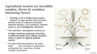
2. Agricultural systems are incredibly
complex, driven by countless
interacting factors.
G NotebookLM
• Farming is not a simple input-output
system. A crop‘s growth and final yield
are the result of a dynamic interplay
between genetics, soil conditions, weather
patterns, and management decisions.
• This ’Soil-Plant—Atmosphere Continuum’
involves numerous processes occurring
at different levels, from cellular reactions
within a plant to regional weather
events.
• To make informed decisions, we need
tools that can help us understand
and predict the outcomes of these
complex interactions.
Nutrien
t
Upaxe
Wate
r
Uptak
e

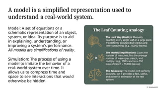
3. A model is a simplified representation used to
understand a real-world system.
G NotebookLM
Model: A set of equations or a
schematic representation of an object,
system, or idea. Its purpose is to aid
in explaining, understanding, or
improving a system's performance.
Ali models are simplifications of reality.
Simulation: The process of using a
model to imitate the behavior of a
real- world system over time. It
allows us to compress time and
space to see interactions that would
otherwise be hidden.

4. G NotebookLM
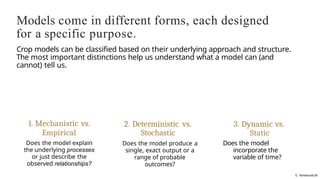
Models come in different forms, each designed
for a specific purpose.
Crop models can be classified based on their underlying approach and structure.
The most important distinctions help us understand what a model can (and
cannot) tell us.
1. Mechanistic vs.
Empirical
Does the model explain
the underlying processes
or just describe the
observed relationships?
2. Deterministic vs.
Stochastic
Does the model produce a
single, exact output or a
range of probable
outcomes?
3. Dynamic vs.
Static
Does the model
incorporate the
variable of time?

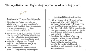
5. The key distinction: Explaining ‘how’ versus describing ‘what’.
G NotebookLM
‹p'p-"'r,'..
Mechanistic (Process-Based) Models
• What they do: Explain not only the
relationship between variables (e.g.,
weather and yield) but also the mechanism
or underlying processes (e.g.,
photosynthesis, respiration).
• How they're built: By analyzing a system
and quantifying its individual processes
(leaf area expansion, tiller production,
etc.) separately, then integrating them.
• Pros: Can be applied over a wider
range of environments. They help
answer "why” questions.
• Cons: More complex and difficult to
build; require deep knowledge of
Empirical (Statistical) Models
• What they do: Quantify relationships
between variables using statistical
techniques like regression. They describe
how variables are related, but not why.
• How they're built: By fitting equations to
a series of measurements made on plants
(e.g., fitting a logistic growth curve to
crop weight data).
• Pros: Easier to build and often very
accurate within the conditions from
which they were derived.
• Cons: Highly site- and condition-
specific. Cannot be reliably used
outside the environment in which they
were developed.

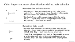
6. Other important model classifications define their behavior.
G NotebookLM
A B
A
Deterministi
c
Stochasti
c
Dynami
c
Stati
c
Deterministic vs. Stochastic Models
• Deterministic: These models estimate an exact value for the
output. For a given set of inputs, the output will always be
the same. There is no element of randomness.
• Stochastic: These models incorporate probability. For a given
set of inputs, they produce a range of possible outputs,
each with an associated probability.
Dynamic vs. Static Models
• Dynamic: Time is included as a critical variable. These models
describe how a system changes over time (e.g., calculating crop
growth on a daily basis from planting to harvest).
• Static: Time is not included as a variable. These models represent
a system at a single point in time, with variables remaining
constant. They are often components within larger dynamic
models.

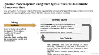
7. Dynamic models operate using three types of variables to simulate
change over time.
G NotebookLM
Crop simulation models use sets of differential equations to calculate changes in the crop and its environment,
typically from planting to harvest. This is done by tracking three kinds of variables:
Driving
Variables
External factors that affect
the system. Their values
must be continuously
monitored.
Examples: Oai/y weather data
like temperature, rainfall, and
solar radiation.
SYSTEM STATE
State Variables: Quantities that define the
state of the system at any given time.
Examples: P/ant biomass, number of leaves,
amount
of nitrogen in the so/’J, soil water content.
Rate Variables
Rate Variables: The rate of change in state
variables, representing the flow of materials or
energy. They are calculated from driving and state
variables.
Examples. Rate of biomass growth per day, rate of
water

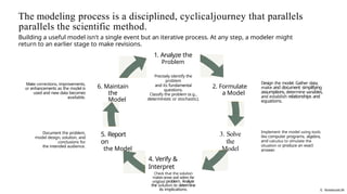
8. The modeling process is a disciplined, cyclicaljourney that parallels
parallels the scientific method.
G NotebookLM
Building a useful model isn't a single event but an iterative process. At any step, a modeler might
return to an earlier stage to make revisions.
1. Analyze the
Problem
Make corrections, improvements,
or enhancements as the model is
used and new data becomes
available.
Document the problem,
model design, solution, and
conclusions for
the intended audience.
6. Maintain
the
Model
5. Report
on
the Model
Precisely identify the
problem
and its fundamental
questions.
Classify the problem (e.g.,
deterministic or stochastic).
4. Verify &
Interpret
Check that the solution
makes sense and solves the
original problem. Analyze
the solution to determine
its implications.
2. Formulate
a Model
3. Solve
the
Model
Design the model. Gather data,
make and document simplifying
assumptions, determine variables,
and establish relationships and
equations.
Implement the model using tools
like computer programs, algebra,
and calculus to slmulate the
situation or produce an exact
answer.

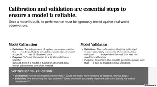
9. Calibration and validation are essential steps to
ensure a model is reliable.
Once a model is built, its performance must be rigorously tested against real-world
observations.
Model Calibration
• Definition: The adjustment of system parameters within
the model so that its simulation results closely match
a specific set of observed data.
• Purpose: To “tune’ the model to a local condition or
specific
dataset. Even if a model is based on observed data,
minor adjustments are often needed.
Model Validation
• Definition: The confirmation that the calibrated
model accurately represents the real situation,
using an independent dataset that was not
used for calibration.
• Purpose: To confirm the model's predictive power and
that it can be trusted in new scenarios.

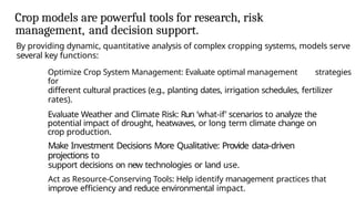
10. Crop models are powerful tools for research, risk
management, and decision support.
By providing dynamic, quantitative analysis of complex cropping systems, models serve
several key functions:
Optimize Crop System Management: Evaluate optimal management strategies
for
different cultural practices (e.g., planting dates, irrigation schedules, fertilizer
rates).
Evaluate Weather and Climate Risk: Run ’what-if’ scenarios to analyze the
potential impact of drought, heatwaves, or long term climate change on
crop production.
Make Investment Decisions More Qualitative: Provide data-driven
projections to
support decisions on new technologies or land use.
Act as Resource-Conserving Tools: Help identify management practices that
improve efficiency and reduce environmental impact.

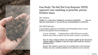
11. Case Study: The Soil Test Crop Response (STCR)
approach uses modeling to prescribe precise
fertilizer doses.
The Problem:
Fertilizer is a costly input. Imbalanced use reduces profitability and can
harmthe environment. A “one-size-fits-all” recommendation is inefficient.
The STCR Solution:
A quantitative approach to fertilizer recommendation that is more
precise than genera! recommendations.
Concept: Developed by Ramamoorthy in 1987, STCR aims to provide
fertilizer doses based on specific soil test values to achieve a pre-defined
Goal: To create a balance between the nutrients supplied by the soil and the
nutrients applied as fertilizer to meet the crop's exact needs for a desired
production level.
Benefit: This method is unique because it provides both a soil-test-based
fertilizer dose and a realistic prediction of the yield that can be achieved.
G NotebookLtVi

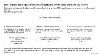
12. The Targeted Yield equation calculates fertilizer needs based on three key factors.
G NotebookLM
To determine the precise fertilizer dose for a specific yield target, the STCR model requires several pieces of information
derived
from field experiments:
Key Inputs for the Equation
1. Nutrient Requirement (NR)
The kilograms of a specific nutrient
(e.g., Nitrogen) required to produce
one quintal (100 kg) of grain.
Nutrient requirement (kg of
nutrient)
Per quintal of grain
Production
2. Percent Contribution from Soil (C.S)
The efficiency with which the available
nutrients already in the soil are taken up by
the crop.
Percent Contribution from soil
to total Nutrient uptake
(C.S)
3. Percent Contribution from Fertilizer (C.F)
The efficiency with which the nutrients
from applied fertilizer are taken up by the
crop.
Percent nutrient contribution
from fertilizer to total uptake
(C.F)
The Logic: The model calculates the total nutrient gap between what the crop needs for the target yield and what the
soil can supply on its own. It then recommends a fertilizer dose to fill that gap, accounting for the efficiency of the
fertilizer itself.

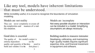
13. Like any tool, models have inherent limitations
that must be understood.
While incredibly useful, it is crucial to recognize the boundaries of simulation
modeling.
G NotebookLM
Models are not reality
They can never completely re-create all
the complexities and nuances of a real-
life situation.
Good data is essential
The quality of the model's output is
entirely dependent on the
quality and quantity of the data used to
build and validate it in the first place ( '
- ' ).
Models are incomplete
Not every possible situation or interaction
can be included in a model. Simplifying
assumptions are always necessary.
Building models is resource-intensive
Developing, calibrating, and maintaining
high- quality models requires significant
expertise, time, and financial investment
in equipment and software.

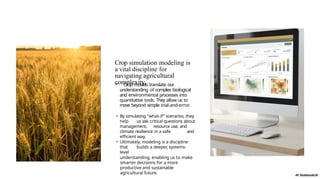
14. Crop simulation modeling is
a vital discipline for
navigating agricultural
complexity.
• Crop models translate our
understanding of complex biological
and environmental processes into
quantitative tools. They allow us to
move beyond simple trial-and-error.
• By simulating "what-if” scenarios, they
help us ask critical questions about
management, resource use, and
climate resilience in a safe and
efficient way.
• Ultimately, modeling is a discipline
that builds a deeper, systems-
level
understanding, enabling us to make
smarter decisions for a more
productive and sustainable
agricultural future.