Downloaded 18 times

![RNA secondary structural data
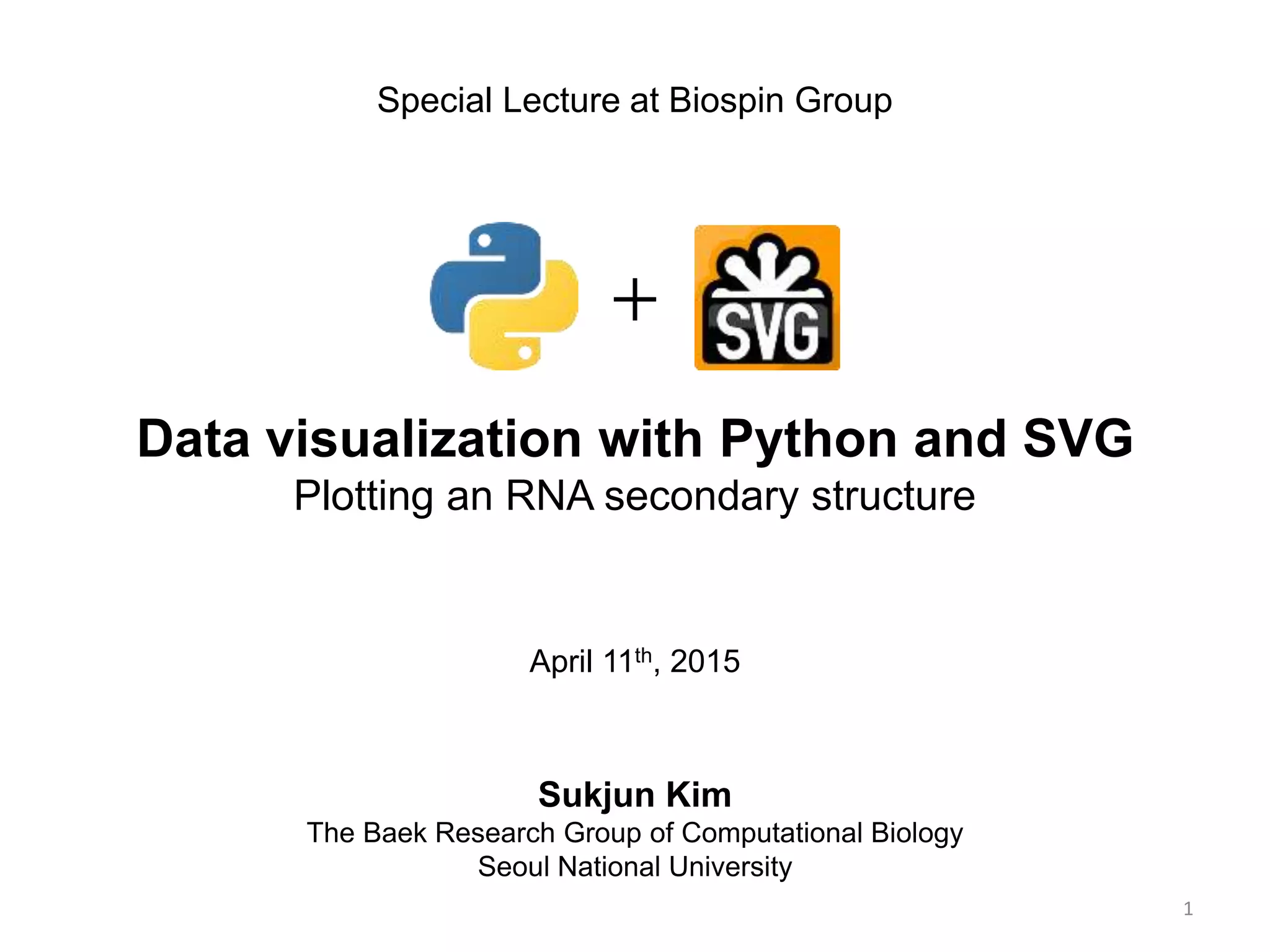
## microRNA structural data
seq = 'CCACCACUUAAACGUGGAUGUACUUGCUUUGAAACUAAAGAAGUAAGUGCUUCCAUGUUUUGGUGAUGG'
dotbr = '(((.((((.(((((((((.(((((((((((.........))))))))))).))))))))).)))).)))'
pairs = [(0,68), (1,67), (2,66), (4,64), (5,63), (6,62), ... , (29,39)]
coor = [(69.515,526.033), (69.515,511.033), ... , (84.515,526.033)]
5
RNAplotRNAfoldseq dotbr, pairs coor
How to generate RNA structural data?
(Vienna RNA package, http://www.tbi.univie.ac.at/RNA/)
• seq: RNA sequence.
• dotbr: dot-bracket notation which is used
to define RNA secondary structure.
• pairs: base-pairing information.
• coor: x and y coordinates for nucleotides.
This is our final
image to plot](https://image.slidesharecdn.com/041115sukjunbiospin-150411044238-conversion-gate01/85/Data-visualization-with-Python-and-SVG-5-320.jpg)
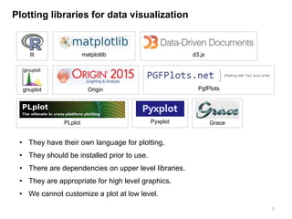
![Writing a SVG tag in python script
6
out = []
out.append('<svg xmlns="http://www.w3.org/2000/svg" version="1.1">n')
## svg elements here
out.append('</svg>n')
open('rna.svg', 'w').write(''.join(out))
<svg xmlns="http://www.w3.org/2000/svg" version="1.1">
</svg>
rna.py
rna.svg
SVG documents basically requires open and close SVG tags](https://image.slidesharecdn.com/041115sukjunbiospin-150411044238-conversion-gate01/85/Data-visualization-with-Python-and-SVG-6-320.jpg)
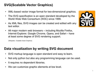
![Drawing phosphate backbone
8
points = ' '.join(['%.3f,%.3f'%(x, y) for x, y in coor])
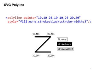
out.append('<polyline points="%s" style="fill:none;
stroke:black; stroke-width:1;"/>n'%(points))
coor = [(69.515,526.033), (69.515,511.033), ... , (84.515,526.033)]
In DNA and RNA, phosphate backbone is regarded as a
skeleton of the molecule. The skeleton will be represented by
SVG <polyline> tag.
We have x and y coordinates of each nucleotide as below.
Using the coordination information, we can specifiy points
attribute of polyline tag.](https://image.slidesharecdn.com/041115sukjunbiospin-150411044238-conversion-gate01/85/Data-visualization-with-Python-and-SVG-8-320.jpg)
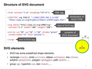
![Drawing base-pairing
10
for i, j in pairs:
x1, y1 = coor[i]
x2, y2 = coor[j]
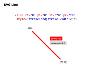
out.append('<line x1="%.3f" y1="%.3f" x2="%.3f" y2="%.3f"
style="stroke:black; stroke-width:1;"/>n'%(x1, y1, x2, y2))
pairs = [(0,68), (1,67), (2,66), (4,64), (5,63), (6,62), ... , (29,39)]
coor = [(69.515,526.033), (69.515,511.033), ... , (84.515,526.033)]
Watson-Crick base pairs occur between A and U, and between
C and G. We will use <line> tag to represent the hydrogen
bonds.
In addition to a coordination information, we also have base-
pairing information in the form of tuple carrying the indexes of
two nucleotides.
From two types of data, base-pairing information can be
visualized as a simple line.](https://image.slidesharecdn.com/041115sukjunbiospin-150411044238-conversion-gate01/85/Data-visualization-with-Python-and-SVG-10-320.jpg)

![Drawing nucleotides
13
A
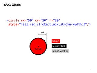
Each nucleotide will be represented by one character text
enclosed with a circle.
seq = 'CCACCACUUAAACGUGGAUGUACUUGCUUUGAAACUAAAGAAGUAAGUGCUUCCAUGUUUUGGUGAUGG'
coor = [(69.515,526.033), (69.515,511.033), ... , (84.515,526.033)]
<text>
<circle>
for i, base in enumerate(seq):
x, y = coor[i]
out.append('<circle cx="%.3f" cy="%.3f" r="%.3f"
style="fill:white; stroke:black; stroke-width:1"/>n'%(x, y, 5))
out.append('<text x="%.3f" y="%.3f" font-size="6" text-
anchor="middle" style="fill:black">%s</text>n'%(x, y+6*0.35, base))
RNA sequence and a coordination information is required.
<text> tag should be written after the <circle> tag.](https://image.slidesharecdn.com/041115sukjunbiospin-150411044238-conversion-gate01/85/Data-visualization-with-Python-and-SVG-13-320.jpg)
![Content of the python script
14
## microRNA structural data
seq = 'CCACCACUUAAACGUGGAUGUACUUGCUUUGAAACUAAAGAAGUAAGUGCUUCCAUGUUUUGGUGAUGG'
dotbr = '(((.((((.(((((((((.(((((((((((.........))))))))))).))))))))).)))).)))'
pairs = [(0, 68), (1, 67), (2, 66), (4, 64), (5, 63), (6, 62), (7, 61), (9, 59), (10, 58), (11, 57), (12, 56), (13, 55), (14,
54), (15, 53), (16, 52), (17, 51), (19, 49), (20, 48), (21, 47), (22, 46), (23, 45), (24, 44), (25, 43), (26, 42), (27, 41),
(28, 40), (29, 39)]
coor =
[(69.515,526.033),(69.515,511.033),(69.515,496.033),(61.778,483.306),(69.515,469.506),(69.515,454.506),(69.515,439.506),(69.
515,424.506),(62.691,412.302),(69.515,400.099),(69.515,385.099),(69.515,370.099),(69.515,355.099),(69.515,340.099),(69.515,3
25.099),(69.515,310.099),(69.515,295.099),(69.515,280.099),(61.778,266.298),(69.515,253.571),(69.515,238.571),(69.515,223.57
1),(69.515,208.571),(69.515,193.571),(69.515,178.571),(69.515,163.571),(69.515,148.571),(69.515,133.571),(69.515,118.571),(6
9.515,103.571),(56.481,95.317),(50.000,81.317),(52.139,66.039),(62.216,54.357),(77.015,50.000),(91.814,54.357),(101.891,66.0
39),(104.030,81.317),(97.549,95.317),(84.515,103.571),(84.515,118.571),(84.515,133.571),(84.515,148.571),(84.515,163.571),(8
4.515,178.571),(84.515,193.571),(84.515,208.571),(84.515,223.571),(84.515,238.571),(84.515,253.571),(92.252,266.298),(84.515
,280.099),(84.515,295.099),(84.515,310.099),(84.515,325.099),(84.515,340.099),(84.515,355.099),(84.515,370.099),(84.515,385.
099),(84.515,400.099),(91.339,412.302),(84.515,424.506),(84.515,439.506),(84.515,454.506),(84.515,469.506),(92.252,483.306),
(84.515,496.033),(84.515,511.033),(84.515,526.033)]
out = []
out.append('<svg xmlns="http://www.w3.org/2000/svg" version="1.1">n')
## [1] phosphate backbone - <polyline> tag
points = ' '.join(['%.3f,%.3f'%(x, y) for x, y in coor])
out.append('<polyline points="%s" style="fill:none; stroke:black; stroke-width:1;"/>n'%(points))
## [2] base-pairing - <line> tag
for i, j in pairs:
x1, y1 = coor[i]
x2, y2 = coor[j]
out.append('<line x1="%.3f" y1="%.3f" x2="%.3f" y2="%.3f" style="stroke:black; stroke-width:1;"/>n'%(x1, y1, x2, y2))
## [3] nucleotide - <circle> and <text> tags
for i, base in enumerate(seq):
x, y = coor[i]
out.append('<circle cx="%.3f" cy="%.3f" r="%.3f" style="fill:white; stroke:black; stroke-width:1"/>n'%(x, y, 5))
out.append('<text x="%.3f" y="%.3f" font-size="6" text-anchor="middle" style="fill:black">%s</text>n'%(x, y+6*0.35,
base))
out.append('</svg>n')
open('rna.svg', 'w').write(''.join(out))](https://image.slidesharecdn.com/041115sukjunbiospin-150411044238-conversion-gate01/85/Data-visualization-with-Python-and-SVG-14-320.jpg)

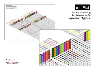
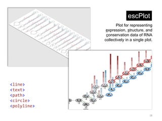
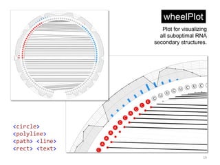


This document discusses using SVG (Scalable Vector Graphics) and Python for data visualization and plotting RNA secondary structure. It provides examples of using different SVG elements like <polyline>, <line>, <circle>, and <text> to represent the phosphate backbone, base pairs, nucleotides, and other features. The document includes an example Python script that generates an SVG file with these elements to plot an RNA secondary structure based on its sequence, dot-bracket notation, and coordinate data.


![제 23회 보아즈(BOAZ) 빅데이터 컨퍼런스 - [MBOAX] : ABSA를 활용한 소비자 반응 분석 기반 운영 효율화 대시보드 설계](https://cdn.slidesharecdn.com/ss_thumbnails/3-1boaz23rdconferencemboax-260203102709-9d519923-thumbnail.jpg?width=640&height=640&fit=bounds)


