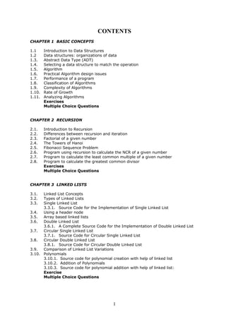
SlideShare a Scribd company logo
1 of 242
Download to read offline
CONTENTS
CHAPTER 1 BASIC CONCEPTS
1.1 Introduction to Data Structures
1.2 Data structures: organizations of data
1.3. Abstract Data Type (ADT)
1.4. Selecting a data structure to match the operation
1.5. Algorithm
1.6. Practical Algorithm design issues
1.7. Performance of a program
1.8. Classification of Algorithms
1.9. Complexity of Algorithms
1.10. Rate of Growth
1.11. Analyzing Algorithms
Exercises
Multiple Choice Questions
CHAPTER 2 RECURSION
2.1. Introduction to Recursion
2.2. Differences between recursion and iteration
2.3. Factorial of a given number
2.4. The Towers of Hanoi
2.5. Fibonacci Sequence Problem
2.6. Program using recursion to calculate the NCR of a given number
2.7. Program to calculate the least common multiple of a given number
2.8. Program to calculate the greatest common divisor
Exercises
Multiple Choice Questions
CHAPTER 3 LINKED LISTS
3.1. Linked List Concepts
3.2. Types of Linked Lists
3.3. Single Linked List
3.3.1. Source Code for the Implementation of Single Linked List
3.4. Using a header node
3.5. Array based linked lists
3.6. Double Linked List
3.6.1. A Complete Source Code for the Implementation of Double Linked List
3.7. Circular Single Linked List
3.7.1. Source Code for Circular Single Linked List
3.8. Circular Double Linked List
3.8.1. Source Code for Circular Double Linked List
3.9. Comparison of Linked List Variations
3.10. Polynomials
3.10.1. Source code for polynomial creation with help of linked list
3.10.2. Addition of Polynomials
3.10.3. Source code for polynomial addition with help of linked list:
Exercise
Multiple Choice Questions
I
CHAPTER 4 STACK AND QUEUE
4.1. Stack
4.1.1. Representation of Stack
4.1.2. Program to demonstrate a stack, using array
4.1.3. Program to demonstrate a stack, using linked list
4.2. Algebraic Expressions
4.3. Converting expressions using Stack
4.3.1. Conversion from infix to postfix
4.3.2. Program to convert an infix to postfix expression
4.3.3. Conversion from infix to prefix
4.3.4. Program to convert an infix to prefix expression
4.3.5. Conversion from postfix to infix
4.3.6. Program to convert postfix to infix expression
4.3.7. Conversion from postfix to prefix
4.3.8. Program to convert postfix to prefix expression
4.3.9. Conversion from prefix to infix
4.3.10. Program to convert prefix to infix expression
4.3.11. Conversion from prefix to postfix
4.3.12. Program to convert prefix to postfix expression
4.4. Evaluation of postfix expression
4.5. Applications of stacks
4.6. Queue
4.6.1. Representation of Queue
4.6.2. Program to demonstrate a Queue using array
4.6.3. Program to demonstrate a Queue using linked list
4.7. Applications of Queue
4.8. Circular Queue
4.8.1. Representation of Circular Queue
4.9. Deque
4.10. Priority Queue
Exercises
Multiple Choice Questions
CHAPTER 5 BINARY TREES
5.1. Trees
5.2. Binary Tree
5.3. Binary Tree Traversal Techniques
5.3.1. Recursive Traversal Algorithms
5.3.2. Building Binary Tree from Traversal Pairs
5.3.3. Binary Tree Creation and Traversal Using Arrays
5.3.4. Binary Tree Creation and Traversal Using Pointers
5.3.5. Non Recursive Traversal Algorithms
5.4. Expression Trees
5.4.1. Converting expressions with expression trees
5.5. Threaded Binary Tree
5.6. Binary Search Tree
5.7. General Trees (m-ary tree)
5.7.1. Converting a m-ary tree (general tree) to a binary tree
5.8. Search and Traversal Techniques for m-ary trees
5.8.1. Depth first search
5.8.2. Breadth first search
5.9. Sparse Matrices
Exercises
Multiple Choice Questions
II
CHAPTER 6 GRAPHS
6.1. Introduction to Graphs
6.2. Representation of Graphs
6.3. Minimum Spanning Tree
6.3.1. Kruskal’s Algorithm
6.3.2. Prim’s Algorithm
6.4. Reachability Matrix
6.5. Traversing a Graph
6.5.1. Breadth first search and traversal
6.5.2. Depth first search and traversal
Exercises
Multiple Choice Questions
CHAPTER 7 SEARCHING AND SORTING
7.1. Linear Search
7.1.1. A non-recursive program for Linear Search
7.1.1. A Recursive program for linear search
7.2. Binary Search
7.1.2. A non-recursive program for binary search
7.1.3. A recursive program for binary search
7.3. Bubble Sort
7.3.1. Program for Bubble Sort
7.4. Selection Sort
7.4.1 Non-recursive Program for selection sort
7.4.2. Recursive Program for selection sort
7.5. Quick Sort
7.5.1. Recursive program for Quick Sort
7.6. Priority Queue and Heap and Heap Sort
7.6.2. Max and Min Heap data structures
7.6.2. Representation of Heap Tree
7.6.3. Operations on heap tree
7.6.4. Merging two heap trees
7.6.5. Application of heap tree
7.7. Heap Sort
7.7.1. Program for Heap Sort
7.8. Priority queue implementation using heap tree
Exercises
Multiple Choice Questions
References and Selected Readings
Index
III
Chapter
1
Basic Concepts
The term data structure is used to describe the way data is stored, and the term
algorithm is used to describe the way data is processed. Data structures and
algorithms are interrelated. Choosing a data structure affects the kind of algorithm
you might use, and choosing an algorithm affects the data structures we use.
An Algorithm is a finite sequence of instructions, each of which has a clear meaning
and can be performed with a finite amount of effort in a finite length of time. No
matter what the input values may be, an algorithm terminates after executing a
finite number of instructions.
1.1. Introduction to Data Structures:
Data structure is a representation of logical relationship existing between individual elements of
data. In other words, a data structure defines a way of organizing all data items that considers
not only the elements stored but also their relationship to each other. The term data structure
is used to describe the way data is stored.
To develop a program of an algorithm we should select an appropriate data structure for that
algorithm. Therefore, data structure is represented as:
Algorithm + Data structure = Program
A data structure is said to be linear if its elements form a sequence or a linear list. The linear
data structures like an array, stacks, queues and linked lists organize data in linear order. A
data structure is said to be non linear if its elements form a hierarchical classification where,
data items appear at various levels.
Trees and Graphs are widely used non-linear data structures. Tree and graph structures
represents hierarchial relationship between individual data elements. Graphs are nothing but
trees with certain restrictions removed.
Data structures are divided into two types:
• Primitive data structures.
• Non-primitive data structures.
Primitive Data Structures are the basic data structures that directly operate upon the
machine instructions. They have different representations on different computers. Integers,
floating point numbers, character constants, string constants and pointers come under this
category.
Non-primitive data structures are more complicated data structures and are derived from
primitive data structures. They emphasize on grouping same or different data items with
relationship between each data item. Arrays, lists and files come under this category. Figure
1.1 shows the classification of data structures.
Lecture Notes Dept. of Information Technology1
Da t a Struc ture s
Pri mit iv e Da t a Struc ture s No n- Pri mit iv e Da t a Struc ture s
Int e ger Flo at Char P o int ers Array s List s File s
No n- Line ar List sLine ar List s
T re e sGra phsQue ue sStac ks
Figure 1. 1. Cla s s if ic at io n of Da t a Struc ture s
1.2. Data structures: Organization of data
The collection of data you work with in a program have some kind of structure or organization.
No matte how complex your data structures are they can be broken down into two fundamental
types:
• Contiguous
• Non-Contiguous.
In contiguous structures, terms of data are kept together in memory (either RAM or in a file).
An array is an example of a contiguous structure. Since each element in the array is located
next to one or two other elements. In contrast, items in a non-contiguous structure and
scattered in memory, but we linked to each other in some way. A linked list is an example of a
non-contiguous data structure. Here, the nodes of the list are linked together using pointers
stored in each node. Figure 1.2 below illustrates the difference between contiguous and non-
contiguous structures.
1 2 3321
(a) Contiguous (b) non-contiguous
Figure 1.2 Contiguous and Non-contiguous structures compared
Contiguous structures:
Contiguous structures can be broken drawn further into two kinds: those that contain data
items of all the same size, and those where the size may differ. Figure 1.2 shows example of
each kind. The first kind is called the array. Figure 1.3(a) shows an example of an array of
numbers. In an array, each element is of the same type, and thus has the same size.
The second kind of contiguous structure is called structure, figure 1.3(b) shows a simple
structure consisting of a person’s name and age. In a struct, elements may be of different data
types and thus may have different sizes.
Lecture Notes Dept. of Information Technology2
For example, a person’s age can be represented with a simple integer that occupies two bytes
of memory. But his or her name, represented as a string of characters, may require many
bytes and may even be of varying length.
Couples with the atomic types (that is, the single data-item built-in types such as integer, float
and pointers), arrays and structs provide all the “mortar” you need to built more exotic form of
data structure, including the non-contiguous forms.
int arr[3] = {1, 2, 3}; struct cust_data
{
int age;
char name[20];
};
cust_data bill= {21, “bill the student”};
1 2 3
(a) Array
21
“bill the student”
(b) struct
Figure 1.3 Examples of contiguous structures.
Non-contiguous structures:
Non-contiguous structures are implemented as a collection of data-items, called nodes, where
each node can point to one or more other nodes in the collection. The simplest kind of non-
contiguous structure is linked list.
A linked list represents a linear, one-dimension type of non-contiguous structure, where there
is only the notation of backwards and forwards. A tree such as shown in figure 1.4(b) is an
example of a two-dimensional non-contiguous structure. Here, there is the notion of up and
down and left and right.
In a tree each node has only one link that leads into the node and links can only go down the
tree. The most general type of non-contiguous structure, called a graph has no such
restrictions. Figure 1.4(c) is an example of a graph.
A B C
(a) Linked List
A
B C
D
GE
F
A
B C
D E F G
(b) Tree (c) graph
Figure 1.4. Examples of non-contiguous structures
Lecture Notes Dept. of Information Technology3
Hybrid structures:
If two basic types of structures are mixed then it is a hybrid form. Then one part contiguous
and another part non-contiguous. For example, figure 1.5 shows how to implement a double–
linked list using three parallel arrays, possibly stored a past from each other in memory.
A B C (a) Conceptual Structure
Figure 1.5. A double linked list via a hybrid data structure
A
B
C
D
3
4
0
1
4
0
1
2
D P N
(b) Hybrid Implementation
List Head
1
2
3
4
The array D contains the data for the list, whereas the array P and N hold the previous and
next “pointers’’. The pointers are actually nothing more than indexes into the D array. For
instance, D[i] holds the data for node i and p[i] holds the index to the node previous to i,
where may or may not reside at position i–1. Like wise, N[i] holds the index to the next node in
the list.
1.3. Abstract Data Type (ADT):
The design of a data structure involves more than just its organization. You also need to plan
for the way the data will be accessed and processed – that is, how the data will be interpreted
actually, non-contiguous structures – including lists, tree and graphs – can be implemented
either contiguously or non- contiguously like wise, the structures that are normally treated as
contiguously - arrays and structures – can also be implemented non-contiguously.
The notion of a data structure in the abstract needs to be treated differently from what ever is
used to implement the structure. The abstract notion of a data structure is defined in terms of
the operations we plan to perform on the data.
Considering both the organization of data and the expected operations on the data, leads to the
notion of an abstract data type. An abstract data type in a theoretical construct that consists of
data as well as the operations to be performed on the data while hiding implementation.
For example, a stack is a typical abstract data type. Items stored in a stack can only be added
and removed in certain order – the last item added is the first item removed. We call these
operations, pushing and popping. In this definition, we haven’t specified have items are stored
on the stack, or how the items are pushed and popped. We have only specified the valid
operations that can be performed.
For example, if we want to read a file, we wrote the code to read the physical file device. That
is, we may have to write the same code over and over again. So we created what is known
Lecture Notes Dept. of Information Technology4
today as an ADT. We wrote the code to read a file and placed it in a library for a programmer to
use.
As another example, the code to read from a keyboard is an ADT. It has a data structure,
character and set of operations that can be used to read that data structure.
To be made useful, an abstract data type (such as stack) has to be implemented and this is
where data structure comes into ply. For instance, we might choose the simple data structure
of an array to represent the stack, and then define the appropriate indexing operations to
perform pushing and popping.
1.4. Selecting a data structure to match the operation:
The most important process in designing a problem involves choosing which data structure to
use. The choice depends greatly on the type of operations you wish to perform.
Suppose we have an application that uses a sequence of objects, where one of the main
operations is delete an object from the middle of the sequence. The code for this is as follows:
void delete (int *seg, int &n, int posn)
// delete the item at position from an array of n elements.
{
if (n)
{
int i=posn;
n--;
while (i < n)
{
seq[i] = seg[i+1];
i++;
}
}
return;
}
This function shifts towards the front all elements that follow the element at position posn. This
shifting involves data movement that, for integer elements, which is too costly. However,
suppose the array stores larger objects, and lots of them. In this case, the overhead for moving
data becomes high. The problem is that, in a contiguous structure, such as an array the logical
ordering (the ordering that we wish to interpret our elements to have) is the same as the
physical ordering (the ordering that the elements actually have in memory).
If we choose non-contiguous representation, however we can separate the logical ordering from
the physical ordering and thus change one without affecting the other. For example, if we store
our collection of elements using a double–linked list (with previous and next pointers), we can
do the deletion without moving the elements, instead, we just modify the pointers in each
node. The code using double linked list is as follows:
void delete (node * beg, int posn)
//delete the item at posn from a list of elements.
{
int i = posn;
node *q = beg;
while (i && q)
{
Lecture Notes Dept. of Information Technology5
i--;
q = q next;
}
if (q)
{ /* not at end of list, so detach P by making previous and
next nodes point to each other */
node *p = q -> prev;
node *n = q -> next;
if (p)
p -> next = n;
if (n)
n -> prev = P;
}
return;
}
The process of detecting a node from a list is independent of the type of data stored in the
node, and can be accomplished with some pointer manipulation as illustrated in figure below:
A C
100 200 300
Initial List
Figure 1.6 Detaching a node from a list
X
A X A
Since very little data is moved during this process, the deletion using linked lists will often be
faster than when arrays are used.
It may seem that linked lists are superior to arrays. But is that always true? There are trade
offs. Our linked lists yield faster deletions, but they take up more space because they require
two extra pointers per element.
1.5. Algorithm
An algorithm is a finite sequence of instructions, each of which has a clear meaning and can be
performed with a finite amount of effort in a finite length of time. No matter what the input
values may be, an algorithm terminates after executing a finite number of instructions. In
addition every algorithm must satisfy the following criteria:
Input: there are zero or more quantities, which are externally supplied;
Output: at least one quantity is produced;
Lecture Notes Dept. of Information Technology6
Definiteness: each instruction must be clear and unambiguous;
Finiteness: if we trace out the instructions of an algorithm, then for all cases the algorithm will
terminate after a finite number of steps;
Effectiveness: every instruction must be sufficiently basic that it can in principle be carried out
by a person using only pencil and paper. It is not enough that each operation be definite, but it
must also be feasible.
In formal computer science, one distinguishes between an algorithm, and a program. A
program does not necessarily satisfy the fourth condition. One important example of such a
program for a computer is its operating system, which never terminates (except for system
crashes) but continues in a wait loop until more jobs are entered.
We represent an algorithm using pseudo language that is a combination of the constructs of a
programming language together with informal English statements.
1.6. Practical Algorithm design issues:
Choosing an efficient algorithm or data structure is just one part of the design process. Next,
will look at some design issues that are broader in scope. There are three basic design goals
that we should strive for in a program:
1. Try to save time (Time complexity).
2. Try to save space (Space complexity).
3. Try to have face.
A program that runs faster is a better program, so saving time is an obvious goal. Like wise, a
program that saves space over a competing program is considered desirable. We want to “save
face” by preventing the program from locking up or generating reams of garbled data.
1.7. Performance of a program:
The performance of a program is the amount of computer memory and time needed to run a
program. We use two approaches to determine the performance of a program. One is
analytical, and the other experimental. In performance analysis we use analytical methods,
while in performance measurement we conduct experiments.
Time Complexity:
The time needed by an algorithm expressed as a function of the size of a problem is called the
TIME COMPLEXITY of the algorithm. The time complexity of a program is the amount of
computer time it needs to run to completion.
The limiting behavior of the complexity as size increases is called the asymptotic time
complexity. It is the asymptotic complexity of an algorithm, which ultimately determines the
size of problems that can be solved by the algorithm.
Space Complexity:
The space complexity of a program is the amount of memory it needs to run to completion. The
space need by a program has the following components:
Lecture Notes Dept. of Information Technology7
Instruction space: Instruction space is the space needed to store the compiled version of the
program instructions.
Data space: Data space is the space needed to store all constant and variable values. Data
space has two components:
• Space needed by constants and simple variables in program.
• Space needed by dynamically allocated objects such as arrays and class instances.
Environment stack space: The environment stack is used to save information needed to
resume execution of partially completed functions.
Instruction Space: The amount of instructions space that is needed depends on factors such
as:
• The compiler used to complete the program into machine code.
• The compiler options in effect at the time of compilation
• The target computer.
1.8. Classification of Algorithms
If ‘n’ is the number of data items to be processed or degree of polynomial or the size of the file
to be sorted or searched or the number of nodes in a graph etc.
1 Next instructions of most programs are executed once or at most only a few times.
If all the instructions of a program have this property, we say that its running time
is a constant.
Log n When the running time of a program is logarithmic, the program gets slightly
slower as n grows. This running time commonly occurs in programs that solve a big
problem by transforming it into a smaller problem, cutting the size by some
constant fraction., When n is a million, log n is a doubled whenever n doubles, log
n increases by a constant, but log n does not double until n increases to n2
.
n When the running time of a program is linear, it is generally the case that a small
amount of processing is done on each input element. This is the optimal situation
for an algorithm that must process n inputs.
n. log n This running time arises for algorithms but solve a problem by breaking it up into
smaller sub-problems, solving them independently, and then combining the
solutions. When n doubles, the running time more than doubles.
n2
When the running time of an algorithm is quadratic, it is practical for use only on
relatively small problems. Quadratic running times typically arise in algorithms that
process all pairs of data items (perhaps in a double nested loop) whenever n
doubles, the running time increases four fold.
n3
Similarly, an algorithm that process triples of data items (perhaps in a triple–
nested loop) has a cubic running time and is practical for use only on small
problems. Whenever n doubles, the running time increases eight fold.
2n
Few algorithms with exponential running time are likely to be appropriate for
practical use, such algorithms arise naturally as “brute–force” solutions to
problems. Whenever n doubles, the running time squares.
Lecture Notes Dept. of Information Technology8
1.9. Complexity of Algorithms
The complexity of an algorithm M is the function f(n) which gives the running time and/or
storage space requirement of the algorithm in terms of the size ‘n’ of the input data. Mostly,
the storage space required by an algorithm is simply a multiple of the data size ‘n’. Complexity
shall refer to the running time of the algorithm.
The function f(n), gives the running time of an algorithm, depends not only on the size ‘n’ of
the input data but also on the particular data. The complexity function f(n) for certain cases
are:
1. Best Case : The minimum possible value of f(n) is called the best case.
2. Average Case : The expected value of f(n).
3. Worst Case : The maximum value of f(n) for any key possible input.
The field of computer science, which studies efficiency of algorithms, is known as analysis of
algorithms.
Algorithms can be evaluated by a variety of criteria. Most often we shall be interested in the
rate of growth of the time or space required to solve larger and larger instances of a problem.
We will associate with the problem an integer, called the size of the problem, which is a
measure of the quantity of input data.
1.10. Rate of Growth
Big–Oh (O), Big–Omega (Ω), Big–Theta (Θ) and Little–Oh
1. T(n) = O(f(n)), (pronounced order of or big oh), says that the growth rate of T(n) is
less than or equal (<) that of f(n)
2. T(n) = Ω(g(n)) (pronounced omega), says that the growth rate of T(n) is greater than
or equal to (>) that of g(n)
3. T(n) = Θ(h(n)) (pronounced theta), says that the growth rate of T(n) equals (=) the
growth rate of h(n) [if T(n) = O(h(n)) and T(n) = Ω (h(n)]
4. T(n) = o(p(n)) (pronounced little oh), says that the growth rate of T(n) is less than the
growth rate of p(n) [if T(n) = O(p(n)) and T(n) ≠ Θ (p(n))].
Some Examples:
2n2
+ 5n – 6 = O(2n
)
2n2
+ 5n – 6 = O(n3
)
2n2
+ 5n – 6 = O(n2
)
2n2
+ 5n – 6 ≠ O(n)
2n2
+ 5n – 6 ≠ Θ(2n
)
2n2
+ 5n – 6 ≠ Θ(n3
)
2n2
+ 5n – 6 = Θ(n2
)
2n2
+ 5n – 6 ≠ Θ(n)
2n2
+ 5n – 6 ≠ Ω(2n
)
2n2
+ 5n – 6 ≠ Ω(n3
)
2n2
+ 5n – 6 = Ω(n2
)
2n2
+ 5n – 6 = Ω(n)
2n2
+ 5n – 6 = o(2n
)
2n2
+ 5n – 6 = o(n3
)
2n2
+ 5n – 6 ≠ o(n2
)
2n2
+ 5n – 6 ≠ o(n)
Lecture Notes Dept. of Information Technology9
1.11. Analyzing Algorithms
Suppose ‘M’ is an algorithm, and suppose ‘n’ is the size of the input data. Clearly the
complexity f(n) of M increases as n increases. It is usually the rate of increase of f(n) we want
to examine. This is usually done by comparing f(n) with some standard functions. The most
common computing times are:
O(1), O(log2 n), O(n), O(n. log2 n), O(n2
), O(n3
), O(2n
), n! and nn
Numerical Comparison of Different Algorithms
The execution time for six of the typical functions is given below:
S.No log n n n. log n n2
n3
2n
1 0 1 1 1 1 2
2 1 2 2 4 8 4
3 2 4 8 16 64 16
4 3 8 24 64 512 256
5 4 16 64 256 4096 65536
Graph of log n, n, n log n, n2
, n3
, 2n
, n! and nn
O(log n) does not depend on the base of the logarithm. To simplify the analysis, the convention
will not have any particular units of time. Thus we throw away leading constants. We will also
throw away low–order terms while computing a Big–Oh running time. Since Big-Oh is an upper
bound, the answer provided is a guarantee that the program will terminate within a certain
time period. The program may stop earlier than this, but never later.
Lecture Notes Dept. of Information Technology10
One way to compare the function f(n) with these standard function is to use the functional ‘O’
notation, suppose f(n) and g(n) are functions defined on the positive integers with the property
that f(n) is bounded by some multiple g(n) for almost all ‘n’. Then,
f(n) = O(g(n))
Which is read as “f(n) is of order g(n)”. For example, the order of complexity for:
• Linear search is O(n)
• Binary search is O(log n)
• Bubble sort is O(n2
)
• Quick sort is O(n log n)
For example, if the first program takes 100n2
milliseconds. While the second taken 5n3
milliseconds. Then might not 5n3
program better than 100n2
program?
As the programs can be evaluated by comparing their running time functions, with constants by
proportionality neglected. So, 5n3
program be better than the 100n2
program.
5 n3
/100 n2
= n/20
for inputs n < 20, the program with running time 5n3
will be faster those the one with running
time 100 n2
.
Therefore, if the program is to be run mainly on inputs of small size, we would indeed prefer
the program whose running time was O(n3
)
However, as ‘n’ gets large, the ratio of the running times, which is n/20, gets arbitrarily larger.
Thus, as the size of the input increases, the O(n3
) program will take significantly more time
than the O(n2
) program. So it is always better to prefer a program whose running time with the
lower growth rate. The low growth rate function’s such as O(n) or O(n log n) are always better.
Exercises
1. Define algorithm.
2. State the various steps in developing algorithms?
3. State the properties of algorithms.
4. Define efficiency of an algorithm?
5. State the various methods to estimate the efficiency of an algorithm.
6. Define time complexity of an algorithm?
7. Define worst case of an algorithm.
8. Define average case of an algorithm.
9. Define best case of an algorithm.
10. Mention the various spaces utilized by a program.
Lecture Notes Dept. of Information Technology11
11. Define space complexity of an algorithm.
12. State the different memory spaces occupied by an algorithm.
Multiple Choice Questions
1. _____ is a step-by-step recipe for solving an instance of problem. [ A ]
A. Algorithm
C. Pseudocode
B. Complexity
D. Analysis
2. ______ is used to describe the algorithm, in less formal language. [ C ]
A. Cannot be defined
C. Pseudocode
B. Natural Language
D. None
3. ______ of an algorithm is the amount of time (or the number of steps)
needed by a program to complete its task.
[ D ]
A. Space Complexity
C. Divide and Conquer
B. Dynamic Programming
D. Time Complexity
4. ______ of a program is the amount of memory used at once by the
algorithm until it completes its execution.
[ C ]
A. Divide and Conquer
C. Space Complexity
B. Time Complexity
D. Dynamic Programming
5. ______ is used to define the worst-case running time of an algorithm. [ A ]
A. Big-Oh notation
C. Complexity
B. Cannot be defined
D. Analysis
Lecture Notes Dept. of Information Technology12
Chapter
2
Recursion
Recursion is deceptively simple in statement but exceptionally
complicated in implementation. Recursive procedures work fine in many
problems. Many programmers prefer recursion through simpler
alternatives are available. It is because recursion is elegant to use
through it is costly in terms of time and space. But using it is one thing
and getting involved with it is another.
In this unit we will look at “recursion” as a programmer who not only
loves it but also wants to understand it! With a bit of involvement it is
going to be an interesting reading for you.
2.1. Introduction to Recursion:
A function is recursive if a statement in the body of the function calls itself. Recursion is
the process of defining something in terms of itself. For a computer language to be
recursive, a function must be able to call itself.
For example, let us consider the function factr() shown below, which computers the
factorial of an integer.
#include <stdio.h>
int factorial (int);
main()
{
int num, fact;
printf (“Enter a positive integer value: ");
scanf (“%d”, &num);
fact = factorial (num);
printf ("n Factorial of %d =%5dn", num, fact);
}
int factorial (int n)
{
int result;
if (n == 0)
return (1);
else
result = n * factorial (n-1);
return (result);
}
A non-recursive or iterative version for finding the factorial is as follows:
factorial (int n)
{
int i, result = 1;
if (n == 0)
Lecture Notes Dept. of Information Technology13
return (result);
else
{
for (i=1; i<=n; i++)
result = result * i;
}
return (result);
}
The operation of the non-recursive version is clear as it uses a loop starting at 1 and
ending at the target value and progressively multiplies each number by the moving
product.
When a function calls itself, new local variables and parameters are allocated storage
on the stack and the function code is executed with these new variables from the start.
A recursive call does not make a new copy of the function. Only the arguments and
variables are new. As each recursive call returns, the old local variables and
parameters are removed from the stack and execution resumes at the point of the
function call inside the function.
When writing recursive functions, you must have a exit condition somewhere to force
the function to return without the recursive call being executed. If you do not have an
exit condition, the recursive function will recurse forever until you run out of stack
space and indicate error about lack of memory, or stack overflow.
2.2. Differences between recursion and iteration:
• Both involve repetition.
• Both involve a termination test.
• Both can occur infinitely.
Iteration Recursion
Iteration explicitly user a repetition
structure.
Recursion achieves repetition through
repeated function calls.
Iteration terminates when the loop
continuation.
Recursion terminates when a base case
is recognized.
Iteration keeps modifying the counter
until the loop continuation condition
fails.
Recursion keeps producing simple
versions of the original problem until
the base case is reached.
Iteration normally occurs within a loop
so the extra memory assigned is
omitted.
Recursion causes another copy of the
function and hence a considerable
memory space’s occupied.
It reduces the processor’s operating
time.
It increases the processor’s operating
time.
2.3. Factorial of a given number:
The operation of recursive factorial function is as follows:
Start out with some natural number N (in our example, 5). The recursive definition is:
n = 0, 0 ! = 1 Base Case
n > 0, n ! = n * (n - 1) ! Recursive Case
Lecture Notes Dept. of Information Technology14
Recursion Factorials:
5! =5 * 4! = 5 *___ = ____ factr(5) = 5 * factr(4) = __
4! = 4 *3! = 4 *___ = ___ factr(4) = 4 * factr(3) = __
3! = 3 * 2! = 3 * ___ = ___ factr(3) = 3 * factr(2) = __
2! = 2 * 1! = 2 * ___ = ___ factr(2) = 2 * factr(1) = __
1! = 1 * 0! = 1 * __ = __ factr(1) = 1 * factr(0) = __
0! = 1 factr(0) = __
5! = 5*4! = 5*4*3! = 5*4*3*2! = 5*4*3*2*1! = 5*4*3*2*1*0! = 5*4*3*2*1*1
=120
We define 0! to equal 1, and we define factorial N (where N > 0), to be N * factorial
(N-1). All recursive functions must have an exit condition, that is a state when it does
not recurse upon itself. Our exit condition in this example is when N = 0.
Tracing of the flow of the factorial () function:
When the factorial function is first called with, say, N = 5, here is what happens:
FUNCTION:
Does N = 0? No
Function Return Value = 5 * factorial (4)
At this time, the function factorial is called again, with N = 4.
FUNCTION:
Does N = 0? No
Function Return Value = 4 * factorial (3)
At this time, the function factorial is called again, with N = 3.
FUNCTION:
Does N = 0? No
Function Return Value = 3 * factorial (2)
At this time, the function factorial is called again, with N = 2.
FUNCTION:
Does N = 0? No
Function Return Value = 2 * factorial (1)
At this time, the function factorial is called again, with N = 1.
FUNCTION:
Does N = 0? No
Function Return Value = 1 * factorial (0)
At this time, the function factorial is called again, with N = 0.
FUNCTION:
Does N = 0? Yes
Function Return Value = 1
Lecture Notes Dept. of Information Technology15
Now, we have to trace our way back up! See, the factorial function was called six
times. At any function level call, all function level calls above still exist! So, when we
have N = 2, the function instances where N = 3, 4, and 5 are still waiting for their
return values.
So, the function call where N = 1 gets retraced first, once the final call returns 0. So,
the function call where N = 1 returns 1*1, or 1. The next higher function call, where N
= 2, returns 2 * 1 (1, because that's what the function call where N = 1 returned). You
just keep working up the chain.
When N = 2, 2 * 1, or 2 was returned.
When N = 3, 3 * 2, or 6 was returned.
When N = 4, 4 * 6, or 24 was returned.
When N = 5, 5 * 24, or 120 was returned.
And since N = 5 was the first function call (hence the last one to be recalled), the value
120 is returned.
2.4. The Towers of Hanoi:
In the game of Towers of Hanoi, there are three towers labeled 1, 2, and 3. The game
starts with n disks on tower A. For simplicity, let n is 3. The disks are numbered from 1
to 3, and without loss of generality we may assume that the diameter of each disk is
the same as its number. That is, disk 1 has diameter 1 (in some unit of measure), disk
2 has diameter 2, and disk 3 has diameter 3. All three disks start on tower A in the
order 1, 2, 3. The objective of the game is to move all the disks in tower 1 to entire
tower 3 using tower 2. That is, at no time can a larger disk be placed on a smaller disk.
Figure 3.11.1, illustrates the initial setup of towers of Hanoi. The figure 3.11.2,
illustrates the final setup of towers of Hanoi.
The rules to be followed in moving the disks from tower 1 tower 3 using tower 2 are as
follows:
• Only one disk can be moved at a time.
• Only the top disc on any tower can be moved to any other tower.
• A larger disk cannot be placed on a smaller disk.
T o w er 1 T o w er 2 T o w er 3
Fig. 3. 11. 1. Init ia l s et up of T o w ers of Ha no i
Lecture Notes Dept. of Information Technology16
T o w er 1 T o w er 2 T o w er 3
Fig 3. 11. 2. F ina l s et up of T o w ers of Ha no i
The towers of Hanoi problem can be easily implemented using recursion. To move the
largest disk to the bottom of tower 3, we move the remaining n – 1 disks to tower 2
and then move the largest disk to tower 3. Now we have the remaining n – 1 disks to
be moved to tower 3. This can be achieved by using the remaining two towers. We can
also use tower 3 to place any disk on it, since the disk placed on tower 3 is the largest
disk and continue the same operation to place the entire disks in tower 3 in order.
The program that uses recursion to produce a list of moves that shows how to
accomplish the task of transferring the n disks from tower 1 to tower 3 is as follows:
#include <stdio.h>
#include <conio.h>
void towers_of_hanoi (int n, char *a, char *b, char *c);
int cnt=0;
int main (void)
{
int n;
printf("Enter number of discs: ");
scanf("%d",&n);
towers_of_hanoi (n, "Tower 1", "Tower 2", "Tower 3");
getch();
}
void towers_of_hanoi (int n, char *a, char *b, char *c)
{
if (n == 1)
{
++cnt;
printf ("n%5d: Move disk 1 from %s to %s", cnt, a, c);
return;
}
else
{
towers_of_hanoi (n-1, a, c, b);
++cnt;
printf ("n%5d: Move disk %d from %s to %s", cnt, n, a, c);
towers_of_hanoi (n-1, b, a, c);
return;
}
}
Lecture Notes Dept. of Information Technology17
Output of the program:
RUN 1:
Enter the number of discs: 3
1: Move disk 1 from tower 1 to tower 3.
2: Move disk 2 from tower 1 to tower 2.
3: Move disk 1 from tower 3 to tower 2.
4: Move disk 3 from tower 1 to tower 3.
5: Move disk 1 from tower 2 to tower 1.
6: Move disk 2 from tower 2 to tower 3.
7: Move disk 1 from tower 1 to tower 3.
RUN 2:
Enter the number of discs: 4
1: Move disk 1 from tower 1 to tower 2.
2: Move disk 2 from tower 1 to tower 3.
3: Move disk 1 from tower 2 to tower 3.
4: Move disk 3 from tower 1 to tower 2.
5: Move disk 1 from tower 3 to tower 1.
6: Move disk 2 from tower 3 to tower 2.
7: Move disk 1 from tower 1 to tower 2.
8: Move disk 4 from tower 1 to tower 3.
9: Move disk 1 from tower 2 to tower 3.
10: Move disk 2 from tower 2 to tower 1.
11: Move disk 1 from tower 3 to tower 1.
12: Move disk 3 from tower 2 to tower 3.
13: Move disk 1 from tower 1 to tower 2.
14: Move disk 2 from tower 1 to tower 3.
15: Move disk 1 from tower 2 to tower 3.
2.5. Fibonacci Sequence Problem:
A Fibonacci sequence starts with the integers 0 and 1. Successive elements in this
sequence are obtained by summing the preceding two elements in the sequence. For
example, third number in the sequence is 0 + 1 = 1, fourth number is 1 + 1= 2, fifth
number is 1 + 2 = 3 and so on. The sequence of Fibonacci integers is given below:
0 1 1 2 3 5 8 13 21 . . . . . . . . .
Lecture Notes Dept. of Information Technology18
A recursive definition for the Fibonacci sequence of integers may be defined as follows:
Fib (n) = n if n = 0 or n = 1
Fib (n) = fib (n-1) + fib (n-2) for n >=2
We will now use the definition to compute fib(5):
fib(5) = fib(4) + fib(3)
fib(3) + fib(2) + fib(3)
fib(2) + fib(1) + fib(2) + fib(3)
fib(1) + fib(0) + fib(1) + fib(2) + fib(3)
1 + 0 + 1 + fib(1) + fib(0) + fib(3)
1 + 0 + 1 + 1 + 0 + fib(2) + fib(1)
1 + 0 + 1 + 1 + 0 + fib(1) + fib(0) + fib(1)
1 + 0 + 1 + 1 + 0 + 1 + 0 + 1 = 5
We see that fib(2) is computed 3 times, and fib(3), 2 times in the above calculations.
We save the values of fib(2) or fib(3) and reuse them whenever needed.
A recursive function to compute the Fibonacci number in the nth
position is given below:
main()
{
clrscr ();
printf (“=nfib(5) is %d”, fib(5));
}
fib(n)
int n;
{
int x;
if (n==0 | | n==1)
return n;
x=fib(n-1) + fib(n-2);
return (x);
}
Output:
fib(5) is 5
Lecture Notes Dept. of Information Technology19
2.6. Program using recursion to calculate the NCR of a given number:
#include<stdio.h>
float ncr (int n, int r);
void main()
{
int n, r, result;
printf(“Enter the value of N and R :”);
scanf(“%d %d”, &n, &r);
result = ncr(n, r);
printf(“The NCR value is %.3f”, result);
}
float ncr (int n, int r)
{
if(r == 0)
return 1;
else
return(n * 1.0 / r * ncr (n-1, r-1));
}
Output:
Enter the value of N and R: 5 2
The NCR value is: 10.00
2.7. Program to calculate the least common multiple of a given number:
#include<stdio.h>
int alone(int a[], int n);
long int lcm(int a[], int n, int prime);
void main()
{
int a[20], status, i, n, prime;
printf (“Enter the limit: “);
scanf(“%d”, &n);
printf (“Enter the numbers : “);
for (i = 0; i < n; i++)
scanf(“%d”, &a[i]);
printf (“The least common multiple is %ld”, lcm(a, n, 2));
}
int alone (int a[], int n);
{
int k;
for (k = 0; k < n; k++)
if (a[k] != 1)
return 0;
return 1;
}
Lecture Notes Dept. of Information Technology20
long int lcm (int a[], int n, int prime)
{
int i, status;
status = 0;
if (allone(a, n))
return 1;
for (i = 0; i < n; i++)
if ((a[i] % prime) == 0)
{
status = 1;
a[i] = a[i] / prime;
}
if (status == 1)
return (prime * lcm(a, n, prime));
else
return (lcm (a, n, prime = (prime == 2) ? prime+1 : prime+2));
}
Output:
Enter the limit: 6
Enter the numbers: 6 5 4 3 2 1
The least common multiple is 60
2.8. Program to calculate the greatest common divisor:
#include<stdio.h>
int check_limit (int a[], int n, int prime);
int check_all (int a[], int n, int prime);
long int gcd (int a[], int n, int prime);
void main()
{
int a[20], stat, i, n, prime;
printf (“Enter the limit: “);
scanf (“%d”, &n);
printf (“Enter the numbers: “);
for (i = 0; i < n; i ++)
scanf (“%d”, &a[i]);
printf (“The greatest common divisor is %ld”, gcd (a, n, 2));
}
int check_limit (int a[], int n, int prime)
{
int i;
for (i = 0; i < n; i++)
if (prime > a[i])
return 1;
return 0;
}
Lecture Notes Dept. of Information Technology21
int check_all (int a[], int n, int prime)
{
int i;
for (i = 0; i < n; i++)
if ((a[i] % prime) != 0)
return 0;
for (i = 0; i < n; i++)
a[i] = a[i] / prime;
return 1;
}
long int gcd (int a[], int n, int prime)
{
int i;
if (check_limit(a, n, prime))
return 1;
if (check_all (a, n, prime))
return (prime * gcd (a, n, prime));
else
return (gcd (a, n, prime = (prime == 2) ? prime+1 : prime+2));
}
Output:
Enter the limit: 5
Enter the numbers: 99 55 22 77 121
The greatest common divisor is 11
Exercises
1. What is the importance of the stopping case in recursive functions?
2. Write a function with one positive integer parameter called n. The function will
write 2^n-1 integers (where ^ is the exponentiation operation). Here are the
patterns of output for various values of n:
n=1: Output is: 1
n=2: Output is: 1 2 1
n=3: Output is: 1 2 1 3 1 2 1
n=4: Output is: 1 2 1 3 1 2 1 4 1 2 1 3 1 2 1
And so on. Note that the output for n always consists of the output for n-1,
followed by n itself, followed by a second copy of the output for n-1.
3. Write a recursive function for the mathematical function:
f(n) = 1 if n = 1
f(n) = 2 * f(n-1) if n >= 2
4. Which method is preferable in general?
a) Recursive method
b) Non-recursive method
5. Write a function using Recursion to print numbers from n to 0.
6. Write a function using Recursion to enter and display a string in reverse and
state whether the string contains any spaces. Don't use arrays/strings.
Lecture Notes Dept. of Information Technology22
7. Write a function using Recursion to check if a number n is prime. (You have to
check whether n is divisible by any number below n)
8. Write a function using Recursion to enter characters one by one until a space is
encountered. The function should return the depth at which the space was
encountered.
Multiple Choice Questions
In a single function declaration, what is the maximum number of
statements that may be recursive calls?
[ ]
A. 1 B. 2
1.
C. n (where n is the argument) D. There is no fixed maximum
What is the maximum depth of recursive calls a function may make? [ ]
A. 1 B. 2
2.
C. n (where n is the argument) D. There is no fixed maximum
Consider the following function:
void super_write_vertical (int number)
{
if (number < 0)
{
printf(“ - ”);
super_write_vertical(abs(number));
}
else if (number < 10)
printf(“%dn”, number);
else
{
super_write_vertical(number/10);
printf(“%dn”, number % 10);
}
}
What values of number are directly handled by the stopping case?
[ ]
A. number < 0 B. number < 10
3.
C. number >= 0 && number < 10 D. number > 10
Consider the following function:
void super_write_vertical(int number)
{
if (number < 0)
{
printf(“ - ”);
super_write_vertical (abs(number));
}
else if (number < 10)
printf(“%dn”, number);
else
{
super_write_vertical(number/10);
printf(“%dn”, number % 10);
}
}
Which call will result in the most recursive calls?
[ ]
A. super_write_vertical(-1023) B. super_write_vertical(0)
4.
C. super_write_vertical(100) D. super_write_vertical(1023)
Lecture Notes Dept. of Information Technology23
Consider this function declaration:
void quiz (int i)
{
if (i > 1)
{
quiz(i / 2);
quiz(i / 2);
}
printf(“ * ”);
}
How many asterisks are printed by the function call quiz(5)?
[ ]
A. 3 B. 4
5.
C. 7 D. 8
In a real computer, what will happen if you make a recursive call without
making the problem smaller?
[ ]
A. The operating system detects the infinite recursion because of the
"repeated state"
B. The program keeps running until you press Ctrl-C
6.
C. The results are non-deterministic
D. The run-time stack overflows, halting the program
When the compiler compiles your program, how is a recursive call
treated differently than a non-recursive function call?
[ ]
A. Parameters are all treated as reference arguments
B. Parameters are all treated as value arguments
7.
C. There is no duplication of local variables
D. None of the above
When a function call is executed, which information is not saved in the
activation record?
[ ]
A. Current depth of recursion.
B. Formal parameters.
8.
C. Location where the function should return when done.
D. Local variables
What technique is often used to prove the correctness of a recursive
function?
[ ]
A. Communitivity. B. Diagonalization.
9.
C. Mathematical induction. D. Matrix Multiplication.
Lecture Notes Dept. of Information Technology24
Chapter
3
LINKED LISTS
In this chapter, the list data structure is presented. This structure can be used
as the basis for the implementation of other data structures (stacks, queues
etc.). The basic linked list can be used without modification in many programs.
However, some applications require enhancements to the linked list design.
These enhancements fall into three broad categories and yield variations on
linked lists that can be used in any combination: circular linked lists, double
linked lists and lists with header nodes.
Linked lists and arrays are similar since they both store collections of data. Array is the
most common data structure used to store collections of elements. Arrays are
convenient to declare and provide the easy syntax to access any element by its index
number. Once the array is set up, access to any element is convenient and fast. The
disadvantages of arrays are:
• The size of the array is fixed. Most often this size is specified at compile
time. This makes the programmers to allocate arrays, which seems "large
enough" than required.
• Inserting new elements at the front is potentially expensive because existing
elements need to be shifted over to make room.
• Deleting an element from an array is not possible.
Linked lists have their own strengths and weaknesses, but they happen to be strong
where arrays are weak. Generally array's allocates the memory for all its elements in
one block whereas linked lists use an entirely different strategy. Linked lists allocate
memory for each element separately and only when necessary.
Here is a quick review of the terminology and rules of pointers. The linked list code will
depend on the following functions:
malloc() is a system function which allocates a block of memory in the "heap" and
returns a pointer to the new block. The prototype of malloc() and other heap functions
are in stdlib.h. malloc() returns NULL if it cannot fulfill the request. It is defined by:
void *malloc (number_of_bytes)
Since a void * is returned the C standard states that this pointer can be converted to
mple,any type. For exa
char *cp;
cp = (char *) malloc (100);
Attempts to get 100 bytes and assigns the starting address to cp. We can also use the
sizeof() function to specify the number of bytes. For example,
int *ip;
ip = (int *) malloc (100*sizeof(int));
Lecture Notes Dept. of Information Technology25
free() is the opposite of malloc(), which de-allocates memory. The argument to free()
is a pointer to a block of memory in the heap — a pointer which was obtained by a
malloc() function. The syntax is:
free (ptr);
The advantage of free() is simply memory management when we no longer need a
block.
3.1. Linked List Concepts:
A linked list is a non-sequential collection of data items. It is a dynamic data structure.
For every data item in a linked list, there is an associated pointer that would give the
memory location of the next data item in the linked list.
The data items in the linked list are not in consecutive memory locations. They may be
anywhere, but the accessing of these data items is easier as each data item contains
the address of the next data item.
Advantages of linked lists:
Linked lists have many advantages. Some of the very important advantages are:
1. Linked lists are dynamic data structures. i.e., they can grow or shrink during
the execution of a program.
2. Linked lists have efficient memory utilization. Here, memory is not pre-
allocated. Memory is allocated whenever it is required and it is de-allocated
(removed) when it is no longer needed.
3. Insertion and Deletions are easier and efficient. Linked lists provide flexibility
in inserting a data item at a specified position and deletion of the data item
from the given position.
4. Many complex applications can be easily carried out with linked lists.
Disadvantages of linked lists:
1. It consumes more space because every node requires a additional pointer to
store address of the next node.
2. Searching a particular element in list is difficult and also time consuming.
3.2. Types of Linked Lists:
Basically we can put linked lists into the following four items:
1. Single Linked List.
2. Double Linked List.
3. Circular Linked List.
4. Circular Double Linked List.
A single linked list is one in which all nodes are linked together in some sequential
manner. Hence, it is also called as linear linked list.
Lecture Notes Dept. of Information Technology26
A double linked list is one in which all nodes are linked together by multiple links which
helps in accessing both the successor node (next node) and predecessor node
(previous node) from any arbitrary node within the list. Therefore each node in a
double linked list has two link fields (pointers) to point to the left node (previous) and
the right node (next). This helps to traverse in forward direction and backward
direction.
A circular linked list is one, which has no beginning and no end. A single linked list can
be made a circular linked list by simply storing address of the very first node in the link
field of the last node.
A circular double linked list is one, which has both the successor pointer and
predecessor pointer in the circular manner.
Comparison between array and linked list:
ARRAY LINKED LIST
Size of an array is fixed Size of a list is not fixed
Memory is allocated from stack Memory is allocated from heap
It is necessary to specify the number of
elements during declaration (i.e., during
compile time).
It is not necessary to specify the
number of elements during declaration
(i.e., memory is allocated during run
time).
It occupies less memory than a linked
list for the same number of elements.
It occupies more memory.
Inserting new elements at the front is
potentially expensive because existing
elements need to be shifted over to
make room.
Inserting a new element at any position
can be carried out easily.
Deleting an element from an array is
not possible.
Deleting an element is possible.
Trade offs between linked lists and arrays:
FEATURE ARRAYS LINKED LISTS
Sequential access efficient efficient
Random access efficient inefficient
Resigning inefficient efficient
Element rearranging inefficient efficient
Overhead per elements none 1 or 2 links
Lecture Notes Dept. of Information Technology27
Applications of linked list:
1. Linked lists are used to represent and manipulate polynomial. Polynomials are
expression containing terms with non zero coefficient and exponents. For
example:
P(x) = a0 Xn
+ a1 Xn-1
+ …… + an-1 X + an
2. Represent very large numbers and operations of the large number such as
addition, multiplication and division.
3. Linked lists are to implement stack, queue, trees and graphs.
4. Implement the symbol table in compiler construction
3.3. Single Linked List:
A linked list allocates space for each element separately in its own block of memory
called a "node". The list gets an overall structure by using pointers to connect all its
nodes together like the links in a chain. Each node contains two fields; a "data" field to
store whatever element, and a "next" field which is a pointer used to link to the next
node. Each node is allocated in the heap using malloc(), so the node memory
continues to exist until it is explicitly de-allocated using free(). The front of the list is a
pointer to the “start” node.
A single linked list is shown in figure 3.2.1.
100
10 200 20 300 30 400 40 X
100 200 300 400
start
Figure 3.2.1. Single Linked List
HEAPSTACK
The next field of the
last node is NULL.
The start
pointer holds
the address
of the first
node of the
list.
Each node stores
the data.
Stores the next
node address.
The beginning of the linked list is stored in a "start" pointer which points to the first
node. The first node contains a pointer to the second node. The second node contains a
pointer to the third node, ... and so on. The last node in the list has its next field set to
NULL to mark the end of the list. Code can access any node in the list by starting at the
start and following the next pointers.
The start pointer is an ordinary local pointer variable, so it is drawn separately on the
left top to show that it is in the stack. The list nodes are drawn on the right to show
that they are allocated in the heap.
Lecture Notes Dept. of Information Technology28
Implementation of Single Linked List:
Before writing the code to build the above list, we need to create a start node, used to
create and access other nodes in the linked list. The following structure definition will
do (see figure 3.2.2):
• Creating a structure with one data item and a next pointer, which will be
pointing to next node of the list. This is called as self-referential structure.
• Initialise the start pointer to be NULL.
NULL
start
Figure 3.2.2. Structure definition, single link node and empty list
Empty list:
struct slinklist
{
int data;
struct slinklist* next;
};
typedef struct slinklist node;
node *start = NULL;
data nextnode:
The basic operations in a single linked list are:
• Creation.
• Insertion.
• Deletion.
• Traversing.
Creating a node for Single Linked List:
Creating a singly linked list starts with creating a node. Sufficient memory has to be
allocated for creating a node. The information is stored in the memory, allocated by
using the malloc() function. The function getnode(), is used for creating a node, after
allocating memory for the structure of type node, the information for the item (i.e.,
data) has to be read from the user, set next field to NULL and finally returns the
address of the node. Figure 3.2.3 illustrates the creation of a node for single linked list.
node* getnode()
{
node* newnode;
newnode = (node *) malloc(sizeof(node));
printf("n Enter data: ");
scanf("%d", &newnode -> data);
newnode -> next = NULL;
return newnode;
}
10 X
newnode
100
Figure 3.2.3. new node with a value of 10
Lecture Notes Dept. of Information Technology29
Creating a Singly Linked List with ‘n’ number of nodes:
The following steps are to be followed to create ‘n’ number of nodes:
• Get the new node using getnode().
newnode = getnode();
• If the list is empty, assign new node as start.
start = newnode;
• If the list is not empty, follow the steps given below:
• The next field of the new node is made to point the first node (i.e.
start node) in the list by assigning the address of the first node.
• The start pointer is made to point the new node by assigning the
address of the new node.
• Repeat the above steps ‘n’ times.
Figure 3.2.4 shows 4 items in a single linked list stored at different locations in
memory.
100
10 200 20 300 30 400 40 X
100 200 300 400
start
Figure 3.2.4. Single Linked List with 4 nodes
The function createlist(), is used to create ‘n’ number of nodes:
vo id createlist(int n)
{
int i;
no de * new no de;
no de *tem p;
for(i = 0; i < n ; i+ +)
{
new no de = getno de();
if(start = = NULL)
{
start = new no de;
}
else
{
tem p = start;
w hile(tem p -> next != NULL)
tem p = tem p -> next;
tem p -> next = new no de;
}
}
}
Lecture Notes Dept. of Information Technology30
Insertion of a Node:
One of the most primitive operations that can be done in a singly linked list is the
insertion of a node. Memory is to be allocated for the new node (in a similar way that is
done while creating a list) before reading the data. The new node will contain empty
data field and empty next field. The data field of the new node is then stored with the
information read from the user. The next field of the new node is assigned to NULL. The
new node can then be inserted at three different places namely:
• Inserting a node at the beginning.
• Inserting a node at the end.
• Inserting a node at intermediate position.
Inserting a node at the beginning:
The following steps are to be followed to insert a new node at the beginning of the list:
• Get the new node using getnode().
newnode = getnode();
• If the list is empty then start = newnode.
• If the list is not empty, follow the steps given below:
newnode -> next = start;
start = newnode;
Figure 3.2.5 shows inserting a node into the single linked list at the beginning.
500
10 200 20 300 30 400 40 X
100 200 300 400
start
Figure 3.2.5. Inserting a node at the beginning
5 100
500
The function insert_at_beg(), is used for inserting a node at the beginning
void insert_at_beg()
{
node *newnode;
newnode = getnode();
if(start == NULL)
{
start = newnode;
}
else
{
newnode -> next = start;
start = newnode;
}
}
Lecture Notes Dept. of Information Technology31
Inserting a node at the end:
The following steps are followed to insert a new node at the end of the list:
• Get the new node using getnode()
newnode = getnode();
• If the list is empty then start = newnode.
• If the list is not empty follow the steps given below:
temp = start;
while(temp -> next != NULL)
temp = temp -> next;
temp -> next = newnode;
Figure 3.2.6 shows inserting a node into the single linked list at the end.
100
10 200 20 300 30 400 40 500
100 200 300 400
start
Figure 3.2.6. Inserting a node at the end.
50 X
500
The function insert_at_end(), is used for inserting a node at the end.
void insert_at_end()
{
node *newnode, *temp;
newnode = getnode();
if(start == NULL)
{
start = newnode;
}
else
{
temp = start;
while(temp -> next != NULL)
temp = temp -> next;
temp -> next = newnode;
}
}
Inserting a node at intermediate position:
The following steps are followed, to insert a new node in an intermediate position in the
list:
• Get the new node using getnode().
newnode = getnode();
Lecture Notes Dept. of Information Technology32
• Ensure that the specified position is in between first node and last node. If
not, specified position is invalid. This is done by countnode() function.
• Store the starting address (which is in start pointer) in temp and prev
pointers. Then traverse the temp pointer upto the specified position followed
by prev pointer.
• After reaching the specified position, follow the steps given below:
prev -> next = newnode;
newnode -> next = temp;
• Let the intermediate position be 3.
Figure 3.2.7 shows inserting a node into the single linked list at a specified
intermediate position other than beginning and end.
100
10 200 20 500 30 400 40 X
100 200 300 400
start
Figure 3.2.7. Inserting a node at an intermediate position.
50 300
500
tempprev
new node
The function insert_at_mid(), is used for inserting a node in the intermediate position.
void insert_at_mid()
{
node *newnode, *temp, *prev;
int pos, nodectr, ctr = 1;
newnode = getnode();
printf("n Enter the position: ");
scanf("%d", &pos);
nodectr = countnode(start);
if(pos > 1 && pos < nodectr)
{
temp = prev = start;
while(ctr < pos)
{
prev = temp;
temp = temp -> next;
ctr++;
}
prev -> next = newnode;
newnode -> next = temp;
}
else
{
printf("position %d is not a middle position", pos);
}
}
Lecture Notes Dept. of Information Technology33
Deletion of a node:
Another primitive operation that can be done in a singly linked list is the deletion of a
node. Memory is to be released for the node to be deleted. A node can be deleted from
the list from three different places namely.
• Deleting a node at the beginning.
• Deleting a node at the end.
• Deleting a node at intermediate position.
Deleting a node at the beginning:
The following steps are followed, to delete a node at the beginning of the list:
• If list is empty then display ‘Empty List’ message.
• If the list is not empty, follow the steps given below:
temp = start;
start = start -> next;
free(temp);
Figure 3.2.8 shows deleting a node at the beginning of a single linked list.
200
10 200 20 300 30 400 40 X
100 200 300 400
start
Figure 3.2.8. Deleting a node at the beginning.
temp
The function delete_at_beg(), is used for deleting the first node in the list.
void delete_at_beg()
{
node *temp;
if(start == NULL)
{
printf("n No nodes are exist..");
return ;
}
else
{
temp = start;
start = temp -> next;
free(temp);
printf("n Node deleted ");
}
}
Lecture Notes Dept. of Information Technology34
Deleting a node at the end:
The following steps are followed to delete a node at the end of the list:
• If list is empty then display ‘Empty List’ message.
• If the list is not empty, follow the steps given below:
temp = prev = start;
while(temp -> next != NULL)
{
prev = temp;
temp = temp -> next;
}
prev -> next = NULL;
free(temp);
Figure 3.2.9 shows deleting a node at the end of a single linked list.
100
10 200 20 300 30 X 40 X
100 200 300 400
start
Figure 3.2.9. Deleting a node at the end.
The function delete_at_last(), is used for deleting the last node in the list.
void delete_at_last()
{
node *temp, *prev;
if(start == NULL)
{
printf("n Empty List..");
return ;
}
else
{
temp = start;
prev = start;
while(temp -> next != NULL)
{
prev = temp;
temp = temp -> next;
}
prev -> next = NULL;
free(temp);
printf("n Node deleted ");
}
}
Lecture Notes Dept. of Information Technology35
Deleting a node at Intermediate position:
The following steps are followed, to delete a node from an intermediate position in the
list (List must contain more than two node).
• If list is empty then display ‘Empty List’ message
• If the list is not empty, follow the steps given below.
if(pos > 1 && pos < nodectr)
{
temp = prev = start;
ctr = 1;
while(ctr < pos)
{
prev = temp;
temp = temp -> next;
ctr++;
}
prev -> next = temp -> next;
free(temp);
printf("n node deleted..");
}
Figure 3.2.10 shows deleting a node at a specified intermediate position other than
beginning and end from a single linked list.
100
10 300 20 300 30 400 40 X
100 200 300 400
start
Figure 3.2.10. Deleting a node at an intermediate position.
The function delete_at_mid(), is used for deleting the intermediate node in the list.
void delete_at_mid()
{
int ctr = 1, pos, nodectr;
node *temp, *prev;
if(start == NULL)
{
printf("n Empty List..");
return ;
}
else
{
printf("n Enter position of node to delete: ");
scanf("%d", &pos);
nodectr = countnode(start);
if(pos > nodectr)
{
printf("nThis node doesnot exist");
}
Lecture Notes Dept. of Information Technology36
if(pos > 1 && pos < nodectr)
{
temp = prev = start;
while(ctr < pos)
{
prev = temp;
temp = temp -> next;
ctr ++;
}
prev -> next = temp -> next;
free(temp);
printf("n Node deleted..");
}
else
{
printf("n Invalid position..");
getch();
}
}
}
Traversal and displaying a list (Left to Right):
To display the information, you have to traverse (move) a linked list, node by node
from the first node, until the end of the list is reached. Traversing a list involves the
following steps:
• Assign the address of start pointer to a temp pointer.
• Display the information from the data field of each node.
The function traverse() is used for traversing and displaying the information stored in
the list from left to right.
void traverse()
{
node *temp;
temp = start;
printf("n The contents of List (Left to Right): n");
if(start == NULL )
printf("n Empty List");
else
{
while (temp != NULL)
{
printf("%d ->", temp -> data);
temp = temp -> next;
}
}
printf("X");
}
Alternatively there is another way to traverse and display the information. That is in
reverse order. The function rev_traverse(), is used for traversing and displaying the
information stored in the list from right to left.
Lecture Notes Dept. of Information Technology37
vo id rev_traverse(no de *st)
{
if(st = = NULL)
{
return;
}
else
{
rev_traverse(st -> next);
printf("%d ->", st -> data);
}
}
Counting the Number of Nodes:
The following code will count the number of nodes exist in the list using recursion.
int co untno de(no de *st)
{
if(st = = NULL)
return 0;
else
return(1 + co untno de(st -> next));
}
3.3.1. Source Code for the Implementation of Single Linked List:
# include <stdio.h>
# include <conio.h>
# include <stdlib.h>
struct slinklist
{
int data;
struct slinklist *next;
};
typedef struct slinklist node;
node *start = NULL;
int menu()
{
int ch;
clrscr();
printf("n 1.Create a list ");
printf("n--------------------------");
printf("n 2.Insert a node at beginning ");
printf("n 3.Insert a node at end");
printf("n 4.Insert a node at middle");
printf("n--------------------------");
printf("n 5.Delete a node from beginning");
printf("n 6.Delete a node from Last");
printf("n 7.Delete a node from Middle");
printf("n--------------------------");
printf("n 8.Traverse the list (Left to Right)");
printf("n 9.Traverse the list (Right to Left)");
Lecture Notes Dept. of Information Technology38
printf("n--------------------------");
printf("n 10. Count nodes ");
printf("n 11. Exit ");
printf("nn Enter your choice: ");
scanf("%d",&ch);
return ch;
}
node* getnode()
{
node * newnode;
newnode = (node *) malloc(sizeof(node));
printf("n Enter data: ");
scanf("%d", &newnode -> data);
newnode -> next = NULL;
return newnode;
}
int countnode(node *ptr)
{
int count=0;
while(ptr != NULL)
{
count++;
ptr = ptr -> next;
}
return (count);
}
void createlist(int n)
{
int i;
node *newnode;
node *temp;
for(i = 0; i < n; i++)
{
newnode = getnode();
if(start == NULL)
{
start = newnode;
}
else
{
temp = start;
while(temp -> next != NULL)
temp = temp -> next;
temp -> next = newnode;
}
}
}
void traverse()
{
node *temp;
temp = start;
printf("n The contents of List (Left to Right): n");
if(start == NULL)
{
printf("n Empty List");
return;
}
else
{
Lecture Notes Dept. of Information Technology39
while(temp != NULL)
{
printf("%d-->", temp -> data);
temp = temp -> next;
}
}
printf(" X ");
}
void rev_traverse(node *start)
{
if(start == NULL)
{
return;
}
else
{
rev_traverse(start -> next);
printf("%d -->", start -> data);
}
}
void insert_at_beg()
{
node *newnode;
newnode = getnode();
if(start == NULL)
{
start = newnode;
}
else
{
newnode -> next = start;
start = newnode;
}
}
void insert_at_end()
{
node *newnode, *temp;
newnode = getnode();
if(start == NULL)
{
start = newnode;
}
else
{
temp = start;
while(temp -> next != NULL)
temp = temp -> next;
temp -> next = newnode;
}
}
void insert_at_mid()
{
node *newnode, *temp, *prev;
int pos, nodectr, ctr = 1;
newnode = getnode();
printf("n Enter the position: ");
scanf("%d", &pos);
nodectr = countnode(start);
Lecture Notes Dept. of Information Technology40
if(pos > 1 && pos < nodectr)
{
temp = prev = start;
while(ctr < pos)
{
prev = temp;
temp = temp -> next;
ctr++;
}
prev -> next = newnode;
newnode -> next = temp;
}
else
printf("position %d is not a middle position", pos);
}
void delete_at_beg()
{
node *temp;
if(start == NULL)
{
printf("n No nodes are exist..");
return ;
}
else
{
temp = start;
start = temp -> next;
free(temp);
printf("n Node deleted ");
}
}
void delete_at_last()
{
node *temp, *prev;
if(start == NULL)
{
printf("n Empty List..");
return ;
}
else
{
temp = start;
prev = start;
while(temp -> next != NULL)
{
prev = temp;
temp = temp -> next;
}
prev -> next = NULL;
free(temp);
printf("n Node deleted ");
}
}
void delete_at_mid()
{
int ctr = 1, pos, nodectr;
node *temp, *prev;
if(start == NULL)
{
printf("n Empty List..");
Lecture Notes Dept. of Information Technology41
return ;
}
else
{
printf("n Enter position of node to delete: ");
scanf("%d", &pos);
nodectr = countnode(start);
if(pos > nodectr)
{
printf("nThis node doesnot exist");
}
if(pos > 1 && pos < nodectr)
{
temp = prev = start;
while(ctr < pos)
{
prev = temp;
temp = temp -> next;
ctr ++;
}
prev -> next = temp -> next;
free(temp);
printf("n Node deleted..");
}
else
{
printf("n Invalid position..");
getch();
}
}
}
void main(void)
{
int ch, n;
clrscr();
while(1)
{
ch = menu();
switch(ch)
{
case 1:
if(start == NULL)
{
printf("n Number of nodes you want to create: ");
scanf("%d", &n);
createlist(n);
printf("n List created..");
}
else
printf("n List is already created..");
break;
case 2:
insert_at_beg();
break;
case 3:
insert_at_end();
break;
case 4:
insert_at_mid();
break;
Lecture Notes Dept. of Information Technology42
case 5:
delete_at_beg();
break;
case 6:
delete_at_last();
break;
case 7:
delete_at_mid();
break;
case 8:
traverse();
break;
case 9:
printf("n The contents of List (Right to Left): n");
rev_traverse(start);
printf(" X ");
break;
case 10:
printf("n No of nodes : %d ", countnode(start));
break;
case 11 :
exit(0);
}
getch();
}
}
3.4. Using a header node:
A header node is a special dummy node found at the front of the list. The use of header
node is an alternative to remove the first node in a list. For example, the picture below
shows how the list with data 10, 20 and 30 would be represented using a linked list
without and with a header node:
100
10 200 20 300 30 X
100 200 300
sta rt
Single Linke d List w it ho ut a he a der no de
400
100 10 200 20 300 30 X
400 100 200 300
sta rt
Single Linke d List w it h he a der no de
Note that if your linked lists do include a header node, there is no need for the special
case code given above for the remove operation; node n can never be the first node in
the list, so there is no need to check for that case. Similarly, having a header node can
simplify the code that adds a node before a given node n.
Lecture Notes Dept. of Information Technology43
Note that if you do decide to use a header node, you must remember to initialize an
empty list to contain one (dummy) node, you must remember not to include the
header node in the count of "real" nodes in the list.
It is also useful when information other than that found in each node of the list is
needed. For example, imagine an application in which the number of items in a list is
often calculated. In a standard linked list, the list function to count the number of
nodes has to traverse the entire list every time. However, if the current length is
maintained in a header node, that information can be obtained very quickly.
3.5. Array based linked lists:
Another alternative is to allocate the nodes in blocks. In fact, if you know the maximum
size of a list a head of time, you can pre-allocate the nodes in a single array. The result
is a hybrid structure – an array based linked list. Figure 3.5.1 shows an example of null
terminated single linked list where all the nodes are allocated contiguously in an array.
100
a 200 b 300 c X
100 200 300
start
Conceptual structure
Implementation
Figure 3.5.1. An array based linked list
a
b
c
d
3.6. Double Linked List:
A double linked list is a two-way list in which all nodes will have two links. This helps in
accessing both successor node and predecessor node from the given node position. It
provides bi-directional traversing. Each node contains three fields:
• Left link.
• Data.
• Right link.
The left link points to the predecessor node and the right link points to the successor
node. The data field stores the required data.
Many applications require searching forward and backward thru nodes of a list. For
example searching for a name in a telephone directory would need forward and
backward scanning thru a region of the whole list.
The basic operations in a double linked list are:
• Creation.
• Insertion.
• Deletion.
• Traversing.
Lecture Notes Dept. of Information Technology44
A double linked list is shown in figure 3.3.1.
100
X 10 200 200 30 X
100 200 300
start
Figure 3.3.1. Double Linked List
HEAPSTACK
The right field of the
last node is NULL.
The start
pointer holds
the address
of the first
node of the
list.
Stores the data. Stores the next
node address.
100 20 300
Stores the previous
node address.
The beginning of the double linked list is stored in a "start" pointer which points to the
first node. The first node’s left link and last node’s right link is set to NULL.
The following code gives the structure definition:
NULL
start
Figure 3.4.1. Structure definition, double link node and empty list
Empty list:
struct dlinklist
{
struct dlinklist *left;
int data;
struct dlinklist *right;
};
typedef struct dlinklist node;
node *start = NULL;
left data rightnode:
Creating a node for Double Linked List:
Creating a double linked list starts with creating a node. Sufficient memory has to be
allocated for creating a node. The information is stored in the memory, allocated by
using the malloc() function. The function getnode(), is used for creating a node, after
allocating memory for the structure of type node, the information for the item (i.e.,
data) has to be read from the user and set left field to NULL and right field also set to
NULL (see figure 3.2.2).
node* getnode()
{
node* newnode;
newnode = (node *) malloc(sizeof(node));
printf("n Enter data: ");
scanf("%d", &newnode -> data);
newnode -> left = NULL;
newnode -> right = NULL;
return newnode;
}
X 10 X
newnode
100
Figure 3.4.2. new node with a value of 10
Lecture Notes Dept. of Information Technology45
Creating a Double Linked List with ‘n’ number of nodes:
The following steps are to be followed to create ‘n’ number of nodes:
• Get the new node using getnode().
newnode =getnode();
• If the list is empty then start = newnode.
• If the list is not empty, follow the steps given below:
• The left field of the new node is made to point the previous node.
• The previous nodes right field must be assigned with address of the
new node.
• Repeat the above steps ‘n’ times.
The function createlist(), is used to create ‘n’ number of nodes:
vo id createlist(int n)
{
int i;
no de * new no de;
no de *tem p;
for(i = 0; i < n; i+ +)
{
new no de = getno de();
if(start = = NULL)
{
start = new no de;
}
else
{
tem p = start;
w hile(tem p -> right)
tem p = tem p -> right;
tem p -> right = new no de;
new no de -> left = tem p;
}
}
}
Figure 3.4.3 shows 3 items in a double linked list stored at different locations.
100
X 10 200 200 30 X
100 200 300
start
Figure 3.4.3. Double Linked List with 3 nodes
100 20 300
Lecture Notes Dept. of Information Technology46
Inserting a node at the beginning:
The following steps are to be followed to insert a new node at the beginning of the list:
• Get the new node using getnode().
newnode=getnode();
• If the list is empty then start = newnode.
• If the list is not empty, follow the steps given below:
newnode -> right = start;
start -> left = newnode;
start = newnode;
The function dbl_insert_beg(), is used for inserting a node at the beginning. Figure
3.4.4 shows inserting a node into the double linked list at the beginning.
400
400 10 200 200 30 X
100 200 300
start
Figure 3.4.4. Inserting a node at the beginning
100 20 300
X 40 100
400
Inserting a node at the end:
The following steps are followed to insert a new node at the end of the list:
• Get the new node using getnode()
newnode=getnode();
• If the list is empty then start = newnode.
• If the list is not empty follow the steps given below:
temp = start;
while(temp -> right != NULL)
temp = temp -> right;
temp -> right = newnode;
newnode -> left = temp;
The function dbl_insert_end(), is used for inserting a node at the end. Figure 3.4.5
shows inserting a node into the double linked list at the end.
Lecture Notes Dept. of Information Technology47
100
X 10 200 200 30 400
100 200 300
start
Figure 3.4.5. Inserting a node at the end
100 20 300
300 40 X
400
Inserting a node at an intermediate position:
The following steps are followed, to insert a new node in an intermediate position in the
list:
• Get the new node using getnode().
newnode=getnode();
• Ensure that the specified position is in between first node and last node. If
not, specified position is invalid. This is done by countnode() function.
• Store the starting address (which is in start pointer) in temp and prev
pointers. Then traverse the temp pointer upto the specified position followed
by prev pointer.
• After reaching the specified position, follow the steps given below:
newnode -> left = temp;
newnode -> right = temp -> right;
temp -> right -> left = newnode;
temp -> right = newnode;
The function dbl_insert_mid(), is used for inserting a node in the intermediate
position. Figure 3.4.6 shows inserting a node into the double linked list at a specified
intermediate position other than beginning and end.
100
X 10 400
400 20 300
100
400
200
start
Figure 3.4.6. Inserting a node at an intermediate position
100 40 200
200 30 X
300
Lecture Notes Dept. of Information Technology48
Deleting a node at the beginning:
The following steps are followed, to delete a node at the beginning of the list:
• If list is empty then display ‘Empty List’ message.
• If the list is not empty, follow the steps given below:
temp = start;
start = start -> right;
start -> left = NULL;
free(temp);
The function dbl_delete_beg(), is used for deleting the first node in the list. Figure
3.4.6 shows deleting a node at the beginning of a double linked list.
200
X 10 200 200 30 X
100 200 300
start
Figure 3.4.6. Deleting a node at beginning
X 20 300
Deleting a node at the end:
The following steps are followed to delete a node at the end of the list:
• If list is empty then display ‘Empty List’ message
• If the list is not empty, follow the steps given below:
temp = start;
while(temp -> right != NULL)
{
temp = temp -> right;
}
temp -> left -> right = NULL;
free(temp);
The function dbl_delete_last(), is used for deleting the last node in the list. Figure 3.4.7
shows deleting a node at the end of a double linked list.
100
X 10 200 200 30 X
100 200 300
start
Figure 3.4.7. Deleting a node at the end
100 20 X
Lecture Notes Dept. of Information Technology49
Deleting a node at Intermediate position:
The following steps are followed, to delete a node from an intermediate position in the
list (List must contain more than two nodes).
• If list is empty then display ‘Empty List’ message.
• If the list is not empty, follow the steps given below:
• Get the position of the node to delete.
• Ensure that the specified position is in between first node and last
node. If not, specified position is invalid.
• Then perform the following steps:
if(pos > 1 && pos < nodectr)
{
temp = start;
i = 1;
while(i < pos)
{
temp = temp -> right;
i++;
}
temp -> right -> left = temp -> left;
temp -> left -> right = temp -> right;
free(temp);
printf("n node deleted..");
}
The function delete_at_mid(), is used for deleting the intermediate node in the list.
Figure 3.4.8 shows deleting a node at a specified intermediate position other than
beginning and end from a double linked list.
100
X 10 300 100 30 X
100 200 300
start
Figure 3.4.8 Deleting a node at an intermediate position
100 20 300
Traversal and displaying a list (Left to Right):
To display the information, you have to traverse the list, node by node from the first
node, until the end of the list is reached. The function traverse_left_right() is used for
traversing and displaying the information stored in the list from left to right.
The following steps are followed, to traverse a list from left to right:
• If list is empty then display ‘Empty List’ message.
• If the list is not empty, follow the steps given below:
Lecture Notes Dept. of Information Technology50
temp = start;
while(temp != NULL)
{
print temp -> data;
temp = temp -> right;
}
Traversal and displaying a list (Right to Left):
To display the information from right to left, you have to traverse the list, node by
node from the first node, until the end of the list is reached. The function
traverse_right_left() is used for traversing and displaying the information stored in the
list from right to left. The following steps are followed, to traverse a list from right to
left:
• If list is empty then display ‘Empty List’ message.
• If the list is not empty, follow the steps given below:
temp = start;
while(temp -> right != NULL)
temp = temp -> right;
while(temp != NULL)
{
print temp -> data;
temp = temp -> left;
}
Counting the Number of Nodes:
The following code will count the number of nodes exist in the list (using recursion).
int co untno de(no de *start)
{
if(start = = NULL)
return 0;
else
return(1 + co untno de(start ->right ));
}
3.5. A Complete Source Code for the Implementation of Double Linked List:
#include <stdio.h>
#include <stdlib.h>
#include <conio.h>
struct dlinklist
{
struct dlinklist *left;
int data;
struct dlinklist *right;
};
typedef struct dlinklist node;
node *start = NULL;
Lecture Notes Dept. of Information Technology51
node* getnode()
{
node * newnode;
newnode = (node *) malloc(sizeof(node));
printf("n Enter data: ");
scanf("%d", &newnode -> data);
newnode -> left = NULL;
newnode -> right = NULL;
return newnode;
}
int countnode(node *start)
{
if(start == NULL)
return 0;
else
return 1 + countnode(start -> right);
}
int menu()
{
int ch;
clrscr();
printf("n 1.Create");
printf("n------------------------------");
printf("n 2. Insert a node at beginning ");
printf("n 3. Insert a node at end");
printf("n 4. Insert a node at middle");
printf("n------------------------------");
printf("n 5. Delete a node from beginning");
printf("n 6. Delete a node from Last");
printf("n 7. Delete a node from Middle");
printf("n------------------------------");
printf("n 8. Traverse the list from Left to Right ");
printf("n 9. Traverse the list from Right to Left ");
printf("n------------------------------");
printf("n 10.Count the Number of nodes in the list");
printf("n 11.Exit ");
printf("nn Enter your choice: ");
scanf("%d", &ch);
return ch;
}
void createlist(int n)
{
int i;
node *newnode;
node *temp;
for(i = 0; i < n; i++)
{
newnode = getnode();
if(start == NULL)
start = newnode;
else
{
temp = start;
while(temp -> right)
temp = temp -> right;
temp -> right = newnode;
newnode -> left = temp;
}
}
}
Lecture Notes Dept. of Information Technology52
void traverse_left_to_right()
{
node *temp;
temp = start;
printf("n The contents of List: ");
if(start == NULL )
printf("n Empty List");
else
{
while(temp != NULL)
{
printf("t %d ", temp -> data);
temp = temp -> right;
}
}
}
void traverse_right_to_left()
{
node *temp;
temp = start;
printf("n The contents of List: ");
if(start == NULL)
printf("n Empty List");
else
{
while(temp -> right != NULL)
temp = temp -> right;
}
while(temp != NULL)
{
printf("t%d", temp -> data);
temp = temp -> left;
}
}
void dll_insert_beg()
{
node *newnode;
newnode = getnode();
if(start == NULL)
start = newnode;
else
{
newnode -> right = start;
start -> left = newnode;
start = newnode;
}
}
void dll_insert_end()
{
node *newnode, *temp;
newnode = getnode();
if(start == NULL)
start = newnode;
else
{
temp = start;
while(temp -> right != NULL)
temp = temp -> right;
temp -> right = newnode;
newnode -> left = temp;
}
}
Lecture Notes Dept. of Information Technology53
void dll_insert_mid()
{
node *newnode,*temp;
int pos, nodectr, ctr = 1;
newnode = getnode();
printf("n Enter the position: ");
scanf("%d", &pos);
nodectr = countnode(start);
if(pos - nodectr >= 2)
{
printf("n Position is out of range..");
return;
}
if(pos > 1 && pos < nodectr)
{
temp = start;
while(ctr < pos - 1)
{
temp = temp -> right;
ctr++;
}
newnode -> left = temp;
newnode -> right = temp -> right;
temp -> right -> left = newnode;
temp -> right = newnode;
}
else
printf("position %d of list is not a middle position ", pos);
}
void dll_delete_beg()
{
node *temp;
if(start == NULL)
{
printf("n Empty list");
getch();
return ;
}
else
{
temp = start;
start = start -> right;
start -> left = NULL;
free(temp);
}
}
void dll_delete_last()
{
node *temp;
if(start == NULL)
{
printf("n Empty list");
getch();
return ;
}
else
{
temp = start;
while(temp -> right != NULL)
Lecture Notes Dept. of Information Technology54
temp = temp -> right;
temp -> left -> right = NULL;
free(temp);
temp = NULL;
}
}
void dll_delete_mid()
{
int i = 0, pos, nodectr;
node *temp;
if(start == NULL)
{
printf("n Empty List");
getch();
return;
}
else
{
printf("n Enter the position of the node to delete: ");
scanf("%d", &pos);
nodectr = countnode(start);
if(pos > nodectr)
{
printf("nthis node does not exist");
getch();
return;
}
if(pos > 1 && pos < nodectr)
{
temp = start;
i = 1;
while(i < pos)
{
temp = temp -> right;
i++;
}
temp -> right -> left = temp -> left;
temp -> left -> right = temp -> right;
free(temp);
printf("n node deleted..");
}
else
{
printf("n It is not a middle position..");
getch();
}
}
}
void main(void)
{
int ch, n;
clrscr();
while(1)
{
ch = menu();
switch( ch)
{
case 1 :
printf("n Enter Number of nodes to create: ");
scanf("%d", &n);
createlist(n);
Lecture Notes Dept. of Information Technology55
printf("n List created..");
break;
case 2 :
dll_insert_beg();
break;
case 3 :
dll_insert_end();
break;
case 4 :
dll_insert_mid();
break;
case 5 :
dll_delete_beg();
break;
case 6 :
dll_delete_last();
break;
case 7 :
dll_delete_mid();
break;
case 8 :
traverse_left_to_right();
break;
case 9 :
traverse_right_to_left();
break;
case 10 :
printf("n Number of nodes: %d", countnode(start));
break;
case 11:
exit(0);
}
getch();
}
}
3.7. Circular Single Linked List:
It is just a single linked list in which the link field of the last node points back to the
address of the first node. A circular linked list has no beginning and no end. It is
necessary to establish a special pointer called start pointer always pointing to the first
node of the list. Circular linked lists are frequently used instead of ordinary linked list
because many operations are much easier to implement. In circular linked list no null
pointers are used, hence all pointers contain valid address.
A circular single linked list is shown in figure 3.6.1.
100
10 200 20 300 30 400 40 100
100 200 300 400
start
Figure 3.6.1. Circular Single Linked List
Lecture Notes Dept. of Information Technology56
The basic operations in a circular single linked list are:
• Creation.
• Insertion.
• Deletion.
• Traversing.
Creating a circular single Linked List with ‘n’ number of nodes:
The following steps are to be followed to create ‘n’ number of nodes:
• Get the new node using getnode().
newnode = getnode();
• If the list is empty, assign new node as start.
start = newnode;
• If the list is not empty, follow the steps given below:
temp = start;
while(temp -> next != NULL)
temp = temp -> next;
temp -> next = newnode;
• Repeat the above steps ‘n’ times.
• newnode -> next = start;
The function createlist(), is used to create ‘n’ number of nodes:
Inserting a node at the beginning:
The following steps are to be followed to insert a new node at the beginning of the
circular list:
• Get the new node using getnode().
newnode = getnode();
• If the list is empty, assign new node as start.
start = newnode;
newnode -> next = start;
• If the list is not empty, follow the steps given below:
last = start;
while(last -> next != start)
last = last -> next;
newnode -> next = start;
start = newnode;
last -> next = start;
Lecture Notes Dept. of Information Technology57
The function cll_insert_beg(), is used for inserting a node at the beginning. Figure
3.6.2 shows inserting a node into the circular single linked list at the beginning.
500
10 200 20 300 30 400 40 500
100 200 300 400
start
Figure 3.6.2. Inserting a node at the beginning
5 100
500
Inserting a node at the end:
The following steps are followed to insert a new node at the end of the list:
• Get the new node using getnode().
newnode = getnode();
• If the list is empty, assign new node as start.
start = newnode;
newnode -> next = start;
• If the list is not empty follow the steps given below:
temp = start;
while(temp -> next != start)
temp = temp -> next;
temp -> next = newnode;
newnode -> next = start;
The function cll_insert_end(), is used for inserting a node at the end.
Figure 3.6.3 shows inserting a node into the circular single linked list at the end.
100
10 200 20 300 30 400 40 500
100 200 300 400
start
Figure 3.6.3 Inserting a node at the end.
50 100
500
Lecture Notes Dept. of Information Technology58
Deleting a node at the beginning:
The following steps are followed, to delete a node at the beginning of the list:
• If the list is empty, display a message ‘Empty List’.
• If the list is not empty, follow the steps given below:
last = temp = start;
while(last -> next != start)
last = last -> next;
start = start -> next;
last -> next = start;
• After deleting the node, if the list is empty then start = NULL.
The function cll_delete_beg(), is used for deleting the first node in the list. Figure 3.6.4
shows deleting a node at the beginning of a circular single linked list.
200
10 200 20 300 30 400 40 200
100 200 300 400
start
Figure 3.6.4. Deleting a node at beginning.
temp
Deleting a node at the end:
The following steps are followed to delete a node at the end of the list:
• If the list is empty, display a message ‘Empty List’.
• If the list is not empty, follow the steps given below:
temp = start;
prev = start;
while(temp -> next != start)
{
prev = temp;
temp = temp -> next;
}
prev -> next = start;
• After deleting the node, if the list is empty then start = NULL.
The function cll_delete_last(), is used for deleting the last node in the list.
Lecture Notes Dept. of Information Technology59
Figure 3.6.5 shows deleting a node at the end of a circular single linked list.
100
10 200 20 300 30 100 40 100
100 200 300 400
start
Figure 3.6.5. Deleting a node at the end.
Traversing a circular single linked list from left to right:
The following steps are followed, to traverse a list from left to right:
• If list is empty then display ‘Empty List’ message.
• If the list is not empty, follow the steps given below:
temp = start;
do
{
printf("%d ", temp -> data);
temp = temp -> next;
} while(temp != start);
3.7.1. Source Code for Circular Single Linked List:
# include <stdio.h>
# include <conio.h>
# include <stdlib.h>
struct cslinklist
{
int data;
struct cslinklist *next;
};
typedef struct cslinklist node;
node *start = NULL;
int nodectr;
node* getnode()
{
node * newnode;
newnode = (node *) malloc(sizeof(node));
printf("n Enter data: ");
scanf("%d", &newnode -> data);
newnode -> next = NULL;
return newnode;
}
Lecture Notes Dept. of Information Technology60
int menu()
{
int ch;
clrscr();
printf("n 1. Create a list ");
printf("nn--------------------------");
printf("n 2. Insert a node at beginning ");
printf("n 3. Insert a node at end");
printf("n 4. Insert a node at middle");
printf("nn--------------------------");
printf("n 5. Delete a node from beginning");
printf("n 6. Delete a node from Last");
printf("n 7. Delete a node from Middle");
printf("nn--------------------------");
printf("n 8. Display the list");
printf("n 9. Exit");
printf("nn--------------------------");
printf("n Enter your choice: ");
scanf("%d", &ch);
return ch;
}
void createlist(int n)
{
int i;
node *newnode;
node *temp;
nodectr = n;
for(i = 0; i < n ; i++)
{
newnode = getnode();
if(start == NULL)
{
start = newnode;
}
else
{
temp = start;
while(temp -> next != NULL)
temp = temp -> next;
temp -> next = newnode;
}
}
newnode ->next = start; /* last node is pointing to starting node */
}
void display()
{
node *temp;
temp = start;
printf("n The contents of List (Left to Right): ");
if(start == NULL )
printf("n Empty List");
else
{
do
{
printf("t %d ", temp -> data);
temp = temp -> next;
} while(temp != start);
printf(" X ");
}
}
Lecture Notes Dept. of Information Technology61
void cll_insert_beg()
{
node *newnode, *last;
newnode = getnode();
if(start == NULL)
{
start = newnode;
newnode -> next = start;
}
else
{
last = start;
while(last -> next != start)
last = last -> next;
newnode -> next = start;
start = newnode;
last -> next = start;
}
printf("n Node inserted at beginning..");
nodectr++;
}
void cll_insert_end()
{
node *newnode, *temp;
newnode = getnode();
if(start == NULL )
{
start = newnode;
newnode -> next = start;
}
else
{
temp = start;
while(temp -> next != start)
temp = temp -> next;
temp -> next = newnode;
newnode -> next = start;
}
printf("n Node inserted at end..");
nodectr++;
}
void cll_insert_mid()
{
node *newnode, *temp, *prev;
int i, pos ;
newnode = getnode();
printf("n Enter the position: ");
scanf("%d", &pos);
if(pos > 1 && pos < nodectr)
{
temp = start;
prev = temp;
i = 1;
while(i < pos)
{
prev = temp;
temp = temp -> next;
i++;
}
prev -> next = newnode;
newnode -> next = temp;
Lecture Notes Dept. of Information Technology62
nodectr++;
printf("n Node inserted at middle..");
}
else
{
printf("position %d of list is not a middle position ", pos);
}
}
void cll_delete_beg()
{
node *temp, *last;
if(start == NULL)
{
printf("n No nodes exist..");
getch();
return ;
}
else
{
last = temp = start;
while(last -> next != start)
last = last -> next;
start = start -> next;
last -> next = start;
free(temp);
nodectr--;
printf("n Node deleted..");
if(nodectr == 0)
start = NULL;
}
}
void cll_delete_last()
{
node *temp,*prev;
if(start == NULL)
{
printf("n No nodes exist..");
getch();
return ;
}
else
{
temp = start;
prev = start;
while(temp -> next != start)
{
prev = temp;
temp = temp -> next;
}
prev -> next = start;
free(temp);
nodectr--;
if(nodectr == 0)
start = NULL;
printf("n Node deleted..");
}
}
Lecture Notes Dept. of Information Technology63
void cll_delete_mid()
{
int i = 0, pos;
node *temp, *prev;
if(start == NULL)
{
printf("n No nodes exist..");
getch();
return ;
}
else
{
printf("n Which node to delete: ");
scanf("%d", &pos);
if(pos > nodectr)
{
printf("nThis node does not exist");
getch();
return;
}
if(pos > 1 && pos < nodectr)
{
temp=start;
prev = start;
i = 0;
while(i < pos - 1)
{
prev = temp;
temp = temp -> next ;
i++;
}
prev -> next = temp -> next;
free(temp);
nodectr--;
printf("n Node Deleted..");
}
else
{
printf("n It is not a middle position..");
getch();
}
}
}
void main(void)
{
int result;
int ch, n;
clrscr();
while(1)
{
ch = menu();
switch(ch)
{
case 1 :
if(start == NULL)
{
printf("n Enter Number of nodes to create: ");
scanf("%d", &n);
createlist(n);
printf("nList created..");
}
Lecture Notes Dept. of Information Technology64
else
printf("n List is already Exist..");
break;
case 2 :
cll_insert_beg();
break;
case 3 :
cll_insert_end();
break;
case 4 :
cll_insert_mid();
break;
case 5 :
cll_delete_beg();
break;
case 6 :
cll_delete_last();
break;
case 7 :
cll_delete_mid();
break;
case 8 :
display();
break;
case 9 :
exit(0);
}
getch();
}
}
3.8. Circular Double Linked List:
A circular double linked list has both successor pointer and predecessor pointer in
circular manner. The objective behind considering circular double linked list is to
simplify the insertion and deletion operations performed on double linked list. In
circular double linked list the right link of the right most node points back to the start
node and left link of the first node points to the last node. A circular double linked list is
shown in figure 3.8.1.
100
300 10 200 200 30 100
100 200 300
start
Figure 3.8.1. Circular Double Linked List
100 20 300
The basic operations in a circular double linked list are:
• Creation.
• Insertion.
• Deletion.
• Traversing.
Lecture Notes Dept. of Information Technology65
Data structures
Data structures
Data structures
Data structures
Data structures
Data structures
Data structures
Data structures
Data structures
Data structures
Data structures
Data structures
Data structures
Data structures
Data structures
Data structures
Data structures
Data structures
Data structures
Data structures
Data structures
Data structures
Data structures
Data structures
Data structures
Data structures
Data structures
Data structures
Data structures
Data structures
Data structures
Data structures
Data structures
Data structures
Data structures
Data structures
Data structures
Data structures
Data structures
Data structures
Data structures
Data structures
Data structures
Data structures
Data structures
Data structures
Data structures
Data structures
Data structures
Data structures
Data structures
Data structures
Data structures
Data structures
Data structures
Data structures
Data structures
Data structures
Data structures
Data structures
Data structures
Data structures
Data structures
Data structures
Data structures
Data structures
Data structures
Data structures
Data structures
Data structures
Data structures
Data structures
Data structures
Data structures
Data structures
Data structures
Data structures
Data structures
Data structures
Data structures
Data structures
Data structures
Data structures
Data structures
Data structures
Data structures
Data structures
Data structures
Data structures
Data structures
Data structures
Data structures
Data structures
Data structures
Data structures
Data structures
Data structures
Data structures
Data structures
Data structures
Data structures
Data structures
Data structures
Data structures
Data structures
Data structures
Data structures
Data structures
Data structures
Data structures
Data structures
Data structures
Data structures
Data structures
Data structures
Data structures
Data structures
Data structures
Data structures
Data structures
Data structures
Data structures
Data structures
Data structures
Data structures
Data structures
Data structures
Data structures
Data structures
Data structures
Data structures
Data structures
Data structures
Data structures
Data structures
Data structures
Data structures
Data structures
Data structures
Data structures
Data structures
Data structures
Data structures
Data structures
Data structures
Data structures
Data structures
Data structures
Data structures
Data structures
Data structures
Data structures
Data structures
Data structures
Data structures
Data structures
Data structures
Data structures
Data structures
Data structures
Data structures
Data structures
Data structures
Data structures
Data structures
Data structures
Data structures
Data structures
Data structures
Data structures
Data structures
Data structures
Data structures
Data structures

More Related Content

What's hot

Data structure
Data structureData structure
Data structureMohd Arif
 
Data structure - Graph
Data structure - GraphData structure - Graph
Data structure - GraphMadhu Bala
 
Data Structures - Lecture 9 [Stack & Queue using Linked List]
 Data Structures - Lecture 9 [Stack & Queue using Linked List] Data Structures - Lecture 9 [Stack & Queue using Linked List]
Data Structures - Lecture 9 [Stack & Queue using Linked List]Muhammad Hammad Waseem
 
Application of Data structure
Application of Data structureApplication of Data structure
Application of Data structureDeepika051991
 
Data Structures- Part7 linked lists
Data Structures- Part7 linked listsData Structures- Part7 linked lists
Data Structures- Part7 linked listsAbdullah Al-hazmy
 
Unit 3 graph chapter6
Unit 3  graph chapter6Unit 3  graph chapter6
Unit 3 graph chapter6DrkhanchanaR
 
BINARY TREE REPRESENTATION.ppt
BINARY TREE REPRESENTATION.pptBINARY TREE REPRESENTATION.ppt
BINARY TREE REPRESENTATION.pptSeethaDinesh
 
Terminology of tree
Terminology of treeTerminology of tree
Terminology of treeRacksaviR
 
Introduction to data structure
Introduction to data structure Introduction to data structure
Introduction to data structure NUPOORAWSARMOL
 
Binary Search Tree
Binary Search TreeBinary Search Tree
Binary Search Treesagar yadav
 
What is Link list? explained with animations
What is Link list? explained with animationsWhat is Link list? explained with animations
What is Link list? explained with animationsPratikNaik41
 

What's hot (20)

Data structure
Data structureData structure
Data structure
 
Data structure - Graph
Data structure - GraphData structure - Graph
Data structure - Graph
 
Data Structures - Lecture 9 [Stack & Queue using Linked List]
 Data Structures - Lecture 9 [Stack & Queue using Linked List] Data Structures - Lecture 9 [Stack & Queue using Linked List]
Data Structures - Lecture 9 [Stack & Queue using Linked List]
 
Application of Data structure
Application of Data structureApplication of Data structure
Application of Data structure
 
Graph traversals in Data Structures
Graph traversals in Data StructuresGraph traversals in Data Structures
Graph traversals in Data Structures
 
Data Structures- Part7 linked lists
Data Structures- Part7 linked listsData Structures- Part7 linked lists
Data Structures- Part7 linked lists
 
Unit 3 graph chapter6
Unit 3  graph chapter6Unit 3  graph chapter6
Unit 3 graph chapter6
 
Linked List
Linked ListLinked List
Linked List
 
Binary search tree(bst)
Binary search tree(bst)Binary search tree(bst)
Binary search tree(bst)
 
BINARY TREE REPRESENTATION.ppt
BINARY TREE REPRESENTATION.pptBINARY TREE REPRESENTATION.ppt
BINARY TREE REPRESENTATION.ppt
 
Lec 1 indexing and hashing
Lec 1 indexing and hashing Lec 1 indexing and hashing
Lec 1 indexing and hashing
 
b+ tree
b+ treeb+ tree
b+ tree
 
Relational model
Relational modelRelational model
Relational model
 
Terminology of tree
Terminology of treeTerminology of tree
Terminology of tree
 
Linked list
Linked listLinked list
Linked list
 
Introduction to data structure
Introduction to data structure Introduction to data structure
Introduction to data structure
 
Binary Search Tree
Binary Search TreeBinary Search Tree
Binary Search Tree
 
Binary tree traversal ppt - 02.03.2020
Binary tree traversal   ppt - 02.03.2020Binary tree traversal   ppt - 02.03.2020
Binary tree traversal ppt - 02.03.2020
 
What is Link list? explained with animations
What is Link list? explained with animationsWhat is Link list? explained with animations
What is Link list? explained with animations
 
Hashing
HashingHashing
Hashing
 

Similar to Data structures

Algoithems and data structures
Algoithems and data structuresAlgoithems and data structures
Algoithems and data structuresadamlongs1983
 
Iare ds lecture_notes_2
Iare ds lecture_notes_2Iare ds lecture_notes_2
Iare ds lecture_notes_2RajSingh734307
 
Data Structure and its Fundamentals
Data Structure and its FundamentalsData Structure and its Fundamentals
Data Structure and its FundamentalsHitesh Mohapatra
 
Data_Structure_and_Algorithms_Using_C++ _ Nho Vĩnh Share.pdf
Data_Structure_and_Algorithms_Using_C++ _ Nho Vĩnh Share.pdfData_Structure_and_Algorithms_Using_C++ _ Nho Vĩnh Share.pdf
Data_Structure_and_Algorithms_Using_C++ _ Nho Vĩnh Share.pdfNho Vĩnh
 
Data Structure & Algorithm.pptx
Data Structure & Algorithm.pptxData Structure & Algorithm.pptx
Data Structure & Algorithm.pptxMumtaz
 
Unit.1 Introduction to Data Structuresres
Unit.1 Introduction to Data StructuresresUnit.1 Introduction to Data Structuresres
Unit.1 Introduction to Data Structuresresamplopsurat
 
DATA STRUCTURES - SHORT NOTES
DATA STRUCTURES - SHORT NOTESDATA STRUCTURES - SHORT NOTES
DATA STRUCTURES - SHORT NOTESsuthi
 
Chapter 1 Introduction to Data Structures and Algorithms.pdf
Chapter 1 Introduction to Data Structures and Algorithms.pdfChapter 1 Introduction to Data Structures and Algorithms.pdf
Chapter 1 Introduction to Data Structures and Algorithms.pdfAxmedcarb
 
employee turnover prediction document.docx
employee turnover prediction document.docxemployee turnover prediction document.docx
employee turnover prediction document.docxrohithprabhas1
 
DataStructurePpt.pptx
DataStructurePpt.pptxDataStructurePpt.pptx
DataStructurePpt.pptxssuser031f35
 
Data Structure Question Bank(2 marks)
Data Structure Question Bank(2 marks)Data Structure Question Bank(2 marks)
Data Structure Question Bank(2 marks)pushpalathakrishnan
 
DS Module 1.pptx
DS Module 1.pptxDS Module 1.pptx
DS Module 1.pptxSaralaT3
 
Introduction to Data Structure
Introduction to Data StructureIntroduction to Data Structure
Introduction to Data StructureJazz Jinia Bhowmik
 
DS Module 1.pptx
DS Module 1.pptxDS Module 1.pptx
DS Module 1.pptxsarala9
 

Similar to Data structures (20)

Ds
DsDs
Ds
 
Data structure
Data structureData structure
Data structure
 
Ad
AdAd
Ad
 
Algoithems and data structures
Algoithems and data structuresAlgoithems and data structures
Algoithems and data structures
 
Iare ds lecture_notes_2
Iare ds lecture_notes_2Iare ds lecture_notes_2
Iare ds lecture_notes_2
 
Data Structure and its Fundamentals
Data Structure and its FundamentalsData Structure and its Fundamentals
Data Structure and its Fundamentals
 
Data_Structure_and_Algorithms_Using_C++ _ Nho Vĩnh Share.pdf
Data_Structure_and_Algorithms_Using_C++ _ Nho Vĩnh Share.pdfData_Structure_and_Algorithms_Using_C++ _ Nho Vĩnh Share.pdf
Data_Structure_and_Algorithms_Using_C++ _ Nho Vĩnh Share.pdf
 
Nagaraju
NagarajuNagaraju
Nagaraju
 
Datastructures Notes
Datastructures NotesDatastructures Notes
Datastructures Notes
 
Data Structure & Algorithm.pptx
Data Structure & Algorithm.pptxData Structure & Algorithm.pptx
Data Structure & Algorithm.pptx
 
Unit.1 Introduction to Data Structuresres
Unit.1 Introduction to Data StructuresresUnit.1 Introduction to Data Structuresres
Unit.1 Introduction to Data Structuresres
 
DATA STRUCTURES - SHORT NOTES
DATA STRUCTURES - SHORT NOTESDATA STRUCTURES - SHORT NOTES
DATA STRUCTURES - SHORT NOTES
 
104333 sri vidhya eng notes
104333 sri vidhya eng notes104333 sri vidhya eng notes
104333 sri vidhya eng notes
 
Chapter 1 Introduction to Data Structures and Algorithms.pdf
Chapter 1 Introduction to Data Structures and Algorithms.pdfChapter 1 Introduction to Data Structures and Algorithms.pdf
Chapter 1 Introduction to Data Structures and Algorithms.pdf
 
employee turnover prediction document.docx
employee turnover prediction document.docxemployee turnover prediction document.docx
employee turnover prediction document.docx
 
DataStructurePpt.pptx
DataStructurePpt.pptxDataStructurePpt.pptx
DataStructurePpt.pptx
 
Data Structure Question Bank(2 marks)
Data Structure Question Bank(2 marks)Data Structure Question Bank(2 marks)
Data Structure Question Bank(2 marks)
 
DS Module 1.pptx
DS Module 1.pptxDS Module 1.pptx
DS Module 1.pptx
 
Introduction to Data Structure
Introduction to Data StructureIntroduction to Data Structure
Introduction to Data Structure
 
DS Module 1.pptx
DS Module 1.pptxDS Module 1.pptx
DS Module 1.pptx
 

Recently uploaded

Microscopic Analysis of Ceramic Materials.pptx
Microscopic Analysis of Ceramic Materials.pptxMicroscopic Analysis of Ceramic Materials.pptx
Microscopic Analysis of Ceramic Materials.pptxpurnimasatapathy1234
 
Current Transformer Drawing and GTP for MSETCL
Current Transformer Drawing and GTP for MSETCLCurrent Transformer Drawing and GTP for MSETCL
Current Transformer Drawing and GTP for MSETCLDeelipZope
 
Call Girls Delhi {Jodhpur} 9711199012 high profile service
Call Girls Delhi {Jodhpur} 9711199012 high profile serviceCall Girls Delhi {Jodhpur} 9711199012 high profile service
Call Girls Delhi {Jodhpur} 9711199012 high profile servicerehmti665
 
Sachpazis Costas: Geotechnical Engineering: A student's Perspective Introduction
Sachpazis Costas: Geotechnical Engineering: A student's Perspective IntroductionSachpazis Costas: Geotechnical Engineering: A student's Perspective Introduction
Sachpazis Costas: Geotechnical Engineering: A student's Perspective IntroductionDr.Costas Sachpazis
 
HARMONY IN THE HUMAN BEING - Unit-II UHV-2
HARMONY IN THE HUMAN BEING - Unit-II UHV-2HARMONY IN THE HUMAN BEING - Unit-II UHV-2
HARMONY IN THE HUMAN BEING - Unit-II UHV-2RajaP95
 
Introduction to Microprocesso programming and interfacing.pptx
Introduction to Microprocesso programming and interfacing.pptxIntroduction to Microprocesso programming and interfacing.pptx
Introduction to Microprocesso programming and interfacing.pptxvipinkmenon1
 
Past, Present and Future of Generative AI
Past, Present and Future of Generative AIPast, Present and Future of Generative AI
Past, Present and Future of Generative AIabhishek36461
 
HARMONY IN THE NATURE AND EXISTENCE - Unit-IV
HARMONY IN THE NATURE AND EXISTENCE - Unit-IVHARMONY IN THE NATURE AND EXISTENCE - Unit-IV
HARMONY IN THE NATURE AND EXISTENCE - Unit-IVRajaP95
 
Call Girls Narol 7397865700 Independent Call Girls
Call Girls Narol 7397865700 Independent Call GirlsCall Girls Narol 7397865700 Independent Call Girls
Call Girls Narol 7397865700 Independent Call Girlsssuser7cb4ff
 
Biology for Computer Engineers Course Handout.pptx
Biology for Computer Engineers Course Handout.pptxBiology for Computer Engineers Course Handout.pptx
Biology for Computer Engineers Course Handout.pptxDeepakSakkari2
 
High Profile Call Girls Nagpur Meera Call 7001035870 Meet With Nagpur Escorts
High Profile Call Girls Nagpur Meera Call 7001035870 Meet With Nagpur EscortsHigh Profile Call Girls Nagpur Meera Call 7001035870 Meet With Nagpur Escorts
High Profile Call Girls Nagpur Meera Call 7001035870 Meet With Nagpur EscortsCall Girls in Nagpur High Profile
 
Architect Hassan Khalil Portfolio for 2024
Architect Hassan Khalil Portfolio for 2024Architect Hassan Khalil Portfolio for 2024
Architect Hassan Khalil Portfolio for 2024hassan khalil
 
College Call Girls Nashik Nehal 7001305949 Independent Escort Service Nashik
College Call Girls Nashik Nehal 7001305949 Independent Escort Service NashikCollege Call Girls Nashik Nehal 7001305949 Independent Escort Service Nashik
College Call Girls Nashik Nehal 7001305949 Independent Escort Service NashikCall Girls in Nagpur High Profile
 
VIP Call Girls Service Hitech City Hyderabad Call +91-8250192130
VIP Call Girls Service Hitech City Hyderabad Call +91-8250192130VIP Call Girls Service Hitech City Hyderabad Call +91-8250192130
VIP Call Girls Service Hitech City Hyderabad Call +91-8250192130Suhani Kapoor
 
microprocessor 8085 and its interfacing
microprocessor 8085  and its interfacingmicroprocessor 8085  and its interfacing
microprocessor 8085 and its interfacingjaychoudhary37
 
VICTOR MAESTRE RAMIREZ - Planetary Defender on NASA's Double Asteroid Redirec...
VICTOR MAESTRE RAMIREZ - Planetary Defender on NASA's Double Asteroid Redirec...VICTOR MAESTRE RAMIREZ - Planetary Defender on NASA's Double Asteroid Redirec...
VICTOR MAESTRE RAMIREZ - Planetary Defender on NASA's Double Asteroid Redirec...VICTOR MAESTRE RAMIREZ
 

Recently uploaded (20)

9953056974 Call Girls In South Ex, Escorts (Delhi) NCR.pdf
9953056974 Call Girls In South Ex, Escorts (Delhi) NCR.pdf9953056974 Call Girls In South Ex, Escorts (Delhi) NCR.pdf
9953056974 Call Girls In South Ex, Escorts (Delhi) NCR.pdf
 
Microscopic Analysis of Ceramic Materials.pptx
Microscopic Analysis of Ceramic Materials.pptxMicroscopic Analysis of Ceramic Materials.pptx
Microscopic Analysis of Ceramic Materials.pptx
 
Current Transformer Drawing and GTP for MSETCL
Current Transformer Drawing and GTP for MSETCLCurrent Transformer Drawing and GTP for MSETCL
Current Transformer Drawing and GTP for MSETCL
 
Call Girls Delhi {Jodhpur} 9711199012 high profile service
Call Girls Delhi {Jodhpur} 9711199012 high profile serviceCall Girls Delhi {Jodhpur} 9711199012 high profile service
Call Girls Delhi {Jodhpur} 9711199012 high profile service
 
Sachpazis Costas: Geotechnical Engineering: A student's Perspective Introduction
Sachpazis Costas: Geotechnical Engineering: A student's Perspective IntroductionSachpazis Costas: Geotechnical Engineering: A student's Perspective Introduction
Sachpazis Costas: Geotechnical Engineering: A student's Perspective Introduction
 
🔝9953056974🔝!!-YOUNG call girls in Rajendra Nagar Escort rvice Shot 2000 nigh...
🔝9953056974🔝!!-YOUNG call girls in Rajendra Nagar Escort rvice Shot 2000 nigh...🔝9953056974🔝!!-YOUNG call girls in Rajendra Nagar Escort rvice Shot 2000 nigh...
🔝9953056974🔝!!-YOUNG call girls in Rajendra Nagar Escort rvice Shot 2000 nigh...
 
HARMONY IN THE HUMAN BEING - Unit-II UHV-2
HARMONY IN THE HUMAN BEING - Unit-II UHV-2HARMONY IN THE HUMAN BEING - Unit-II UHV-2
HARMONY IN THE HUMAN BEING - Unit-II UHV-2
 
Introduction to Microprocesso programming and interfacing.pptx
Introduction to Microprocesso programming and interfacing.pptxIntroduction to Microprocesso programming and interfacing.pptx
Introduction to Microprocesso programming and interfacing.pptx
 
Past, Present and Future of Generative AI
Past, Present and Future of Generative AIPast, Present and Future of Generative AI
Past, Present and Future of Generative AI
 
HARMONY IN THE NATURE AND EXISTENCE - Unit-IV
HARMONY IN THE NATURE AND EXISTENCE - Unit-IVHARMONY IN THE NATURE AND EXISTENCE - Unit-IV
HARMONY IN THE NATURE AND EXISTENCE - Unit-IV
 
Call Girls Narol 7397865700 Independent Call Girls
Call Girls Narol 7397865700 Independent Call GirlsCall Girls Narol 7397865700 Independent Call Girls
Call Girls Narol 7397865700 Independent Call Girls
 
Biology for Computer Engineers Course Handout.pptx
Biology for Computer Engineers Course Handout.pptxBiology for Computer Engineers Course Handout.pptx
Biology for Computer Engineers Course Handout.pptx
 
High Profile Call Girls Nagpur Meera Call 7001035870 Meet With Nagpur Escorts
High Profile Call Girls Nagpur Meera Call 7001035870 Meet With Nagpur EscortsHigh Profile Call Girls Nagpur Meera Call 7001035870 Meet With Nagpur Escorts
High Profile Call Girls Nagpur Meera Call 7001035870 Meet With Nagpur Escorts
 
Architect Hassan Khalil Portfolio for 2024
Architect Hassan Khalil Portfolio for 2024Architect Hassan Khalil Portfolio for 2024
Architect Hassan Khalil Portfolio for 2024
 
young call girls in Rajiv Chowk🔝 9953056974 🔝 Delhi escort Service
young call girls in Rajiv Chowk🔝 9953056974 🔝 Delhi escort Serviceyoung call girls in Rajiv Chowk🔝 9953056974 🔝 Delhi escort Service
young call girls in Rajiv Chowk🔝 9953056974 🔝 Delhi escort Service
 
College Call Girls Nashik Nehal 7001305949 Independent Escort Service Nashik
College Call Girls Nashik Nehal 7001305949 Independent Escort Service NashikCollege Call Girls Nashik Nehal 7001305949 Independent Escort Service Nashik
College Call Girls Nashik Nehal 7001305949 Independent Escort Service Nashik
 
VIP Call Girls Service Hitech City Hyderabad Call +91-8250192130
VIP Call Girls Service Hitech City Hyderabad Call +91-8250192130VIP Call Girls Service Hitech City Hyderabad Call +91-8250192130
VIP Call Girls Service Hitech City Hyderabad Call +91-8250192130
 
microprocessor 8085 and its interfacing
microprocessor 8085  and its interfacingmicroprocessor 8085  and its interfacing
microprocessor 8085 and its interfacing
 
VICTOR MAESTRE RAMIREZ - Planetary Defender on NASA's Double Asteroid Redirec...
VICTOR MAESTRE RAMIREZ - Planetary Defender on NASA's Double Asteroid Redirec...VICTOR MAESTRE RAMIREZ - Planetary Defender on NASA's Double Asteroid Redirec...
VICTOR MAESTRE RAMIREZ - Planetary Defender on NASA's Double Asteroid Redirec...
 
Exploring_Network_Security_with_JA3_by_Rakesh Seal.pptx
Exploring_Network_Security_with_JA3_by_Rakesh Seal.pptxExploring_Network_Security_with_JA3_by_Rakesh Seal.pptx
Exploring_Network_Security_with_JA3_by_Rakesh Seal.pptx
 

Data structures

  • 1. CONTENTS CHAPTER 1 BASIC CONCEPTS 1.1 Introduction to Data Structures 1.2 Data structures: organizations of data 1.3. Abstract Data Type (ADT) 1.4. Selecting a data structure to match the operation 1.5. Algorithm 1.6. Practical Algorithm design issues 1.7. Performance of a program 1.8. Classification of Algorithms 1.9. Complexity of Algorithms 1.10. Rate of Growth 1.11. Analyzing Algorithms Exercises Multiple Choice Questions CHAPTER 2 RECURSION 2.1. Introduction to Recursion 2.2. Differences between recursion and iteration 2.3. Factorial of a given number 2.4. The Towers of Hanoi 2.5. Fibonacci Sequence Problem 2.6. Program using recursion to calculate the NCR of a given number 2.7. Program to calculate the least common multiple of a given number 2.8. Program to calculate the greatest common divisor Exercises Multiple Choice Questions CHAPTER 3 LINKED LISTS 3.1. Linked List Concepts 3.2. Types of Linked Lists 3.3. Single Linked List 3.3.1. Source Code for the Implementation of Single Linked List 3.4. Using a header node 3.5. Array based linked lists 3.6. Double Linked List 3.6.1. A Complete Source Code for the Implementation of Double Linked List 3.7. Circular Single Linked List 3.7.1. Source Code for Circular Single Linked List 3.8. Circular Double Linked List 3.8.1. Source Code for Circular Double Linked List 3.9. Comparison of Linked List Variations 3.10. Polynomials 3.10.1. Source code for polynomial creation with help of linked list 3.10.2. Addition of Polynomials 3.10.3. Source code for polynomial addition with help of linked list: Exercise Multiple Choice Questions I
  • 2. CHAPTER 4 STACK AND QUEUE 4.1. Stack 4.1.1. Representation of Stack 4.1.2. Program to demonstrate a stack, using array 4.1.3. Program to demonstrate a stack, using linked list 4.2. Algebraic Expressions 4.3. Converting expressions using Stack 4.3.1. Conversion from infix to postfix 4.3.2. Program to convert an infix to postfix expression 4.3.3. Conversion from infix to prefix 4.3.4. Program to convert an infix to prefix expression 4.3.5. Conversion from postfix to infix 4.3.6. Program to convert postfix to infix expression 4.3.7. Conversion from postfix to prefix 4.3.8. Program to convert postfix to prefix expression 4.3.9. Conversion from prefix to infix 4.3.10. Program to convert prefix to infix expression 4.3.11. Conversion from prefix to postfix 4.3.12. Program to convert prefix to postfix expression 4.4. Evaluation of postfix expression 4.5. Applications of stacks 4.6. Queue 4.6.1. Representation of Queue 4.6.2. Program to demonstrate a Queue using array 4.6.3. Program to demonstrate a Queue using linked list 4.7. Applications of Queue 4.8. Circular Queue 4.8.1. Representation of Circular Queue 4.9. Deque 4.10. Priority Queue Exercises Multiple Choice Questions CHAPTER 5 BINARY TREES 5.1. Trees 5.2. Binary Tree 5.3. Binary Tree Traversal Techniques 5.3.1. Recursive Traversal Algorithms 5.3.2. Building Binary Tree from Traversal Pairs 5.3.3. Binary Tree Creation and Traversal Using Arrays 5.3.4. Binary Tree Creation and Traversal Using Pointers 5.3.5. Non Recursive Traversal Algorithms 5.4. Expression Trees 5.4.1. Converting expressions with expression trees 5.5. Threaded Binary Tree 5.6. Binary Search Tree 5.7. General Trees (m-ary tree) 5.7.1. Converting a m-ary tree (general tree) to a binary tree 5.8. Search and Traversal Techniques for m-ary trees 5.8.1. Depth first search 5.8.2. Breadth first search 5.9. Sparse Matrices Exercises Multiple Choice Questions II
  • 3. CHAPTER 6 GRAPHS 6.1. Introduction to Graphs 6.2. Representation of Graphs 6.3. Minimum Spanning Tree 6.3.1. Kruskal’s Algorithm 6.3.2. Prim’s Algorithm 6.4. Reachability Matrix 6.5. Traversing a Graph 6.5.1. Breadth first search and traversal 6.5.2. Depth first search and traversal Exercises Multiple Choice Questions CHAPTER 7 SEARCHING AND SORTING 7.1. Linear Search 7.1.1. A non-recursive program for Linear Search 7.1.1. A Recursive program for linear search 7.2. Binary Search 7.1.2. A non-recursive program for binary search 7.1.3. A recursive program for binary search 7.3. Bubble Sort 7.3.1. Program for Bubble Sort 7.4. Selection Sort 7.4.1 Non-recursive Program for selection sort 7.4.2. Recursive Program for selection sort 7.5. Quick Sort 7.5.1. Recursive program for Quick Sort 7.6. Priority Queue and Heap and Heap Sort 7.6.2. Max and Min Heap data structures 7.6.2. Representation of Heap Tree 7.6.3. Operations on heap tree 7.6.4. Merging two heap trees 7.6.5. Application of heap tree 7.7. Heap Sort 7.7.1. Program for Heap Sort 7.8. Priority queue implementation using heap tree Exercises Multiple Choice Questions References and Selected Readings Index III
  • 4. Chapter 1 Basic Concepts The term data structure is used to describe the way data is stored, and the term algorithm is used to describe the way data is processed. Data structures and algorithms are interrelated. Choosing a data structure affects the kind of algorithm you might use, and choosing an algorithm affects the data structures we use. An Algorithm is a finite sequence of instructions, each of which has a clear meaning and can be performed with a finite amount of effort in a finite length of time. No matter what the input values may be, an algorithm terminates after executing a finite number of instructions. 1.1. Introduction to Data Structures: Data structure is a representation of logical relationship existing between individual elements of data. In other words, a data structure defines a way of organizing all data items that considers not only the elements stored but also their relationship to each other. The term data structure is used to describe the way data is stored. To develop a program of an algorithm we should select an appropriate data structure for that algorithm. Therefore, data structure is represented as: Algorithm + Data structure = Program A data structure is said to be linear if its elements form a sequence or a linear list. The linear data structures like an array, stacks, queues and linked lists organize data in linear order. A data structure is said to be non linear if its elements form a hierarchical classification where, data items appear at various levels. Trees and Graphs are widely used non-linear data structures. Tree and graph structures represents hierarchial relationship between individual data elements. Graphs are nothing but trees with certain restrictions removed. Data structures are divided into two types: • Primitive data structures. • Non-primitive data structures. Primitive Data Structures are the basic data structures that directly operate upon the machine instructions. They have different representations on different computers. Integers, floating point numbers, character constants, string constants and pointers come under this category. Non-primitive data structures are more complicated data structures and are derived from primitive data structures. They emphasize on grouping same or different data items with relationship between each data item. Arrays, lists and files come under this category. Figure 1.1 shows the classification of data structures. Lecture Notes Dept. of Information Technology1
  • 5. Da t a Struc ture s Pri mit iv e Da t a Struc ture s No n- Pri mit iv e Da t a Struc ture s Int e ger Flo at Char P o int ers Array s List s File s No n- Line ar List sLine ar List s T re e sGra phsQue ue sStac ks Figure 1. 1. Cla s s if ic at io n of Da t a Struc ture s 1.2. Data structures: Organization of data The collection of data you work with in a program have some kind of structure or organization. No matte how complex your data structures are they can be broken down into two fundamental types: • Contiguous • Non-Contiguous. In contiguous structures, terms of data are kept together in memory (either RAM or in a file). An array is an example of a contiguous structure. Since each element in the array is located next to one or two other elements. In contrast, items in a non-contiguous structure and scattered in memory, but we linked to each other in some way. A linked list is an example of a non-contiguous data structure. Here, the nodes of the list are linked together using pointers stored in each node. Figure 1.2 below illustrates the difference between contiguous and non- contiguous structures. 1 2 3321 (a) Contiguous (b) non-contiguous Figure 1.2 Contiguous and Non-contiguous structures compared Contiguous structures: Contiguous structures can be broken drawn further into two kinds: those that contain data items of all the same size, and those where the size may differ. Figure 1.2 shows example of each kind. The first kind is called the array. Figure 1.3(a) shows an example of an array of numbers. In an array, each element is of the same type, and thus has the same size. The second kind of contiguous structure is called structure, figure 1.3(b) shows a simple structure consisting of a person’s name and age. In a struct, elements may be of different data types and thus may have different sizes. Lecture Notes Dept. of Information Technology2
  • 6. For example, a person’s age can be represented with a simple integer that occupies two bytes of memory. But his or her name, represented as a string of characters, may require many bytes and may even be of varying length. Couples with the atomic types (that is, the single data-item built-in types such as integer, float and pointers), arrays and structs provide all the “mortar” you need to built more exotic form of data structure, including the non-contiguous forms. int arr[3] = {1, 2, 3}; struct cust_data { int age; char name[20]; }; cust_data bill= {21, “bill the student”}; 1 2 3 (a) Array 21 “bill the student” (b) struct Figure 1.3 Examples of contiguous structures. Non-contiguous structures: Non-contiguous structures are implemented as a collection of data-items, called nodes, where each node can point to one or more other nodes in the collection. The simplest kind of non- contiguous structure is linked list. A linked list represents a linear, one-dimension type of non-contiguous structure, where there is only the notation of backwards and forwards. A tree such as shown in figure 1.4(b) is an example of a two-dimensional non-contiguous structure. Here, there is the notion of up and down and left and right. In a tree each node has only one link that leads into the node and links can only go down the tree. The most general type of non-contiguous structure, called a graph has no such restrictions. Figure 1.4(c) is an example of a graph. A B C (a) Linked List A B C D GE F A B C D E F G (b) Tree (c) graph Figure 1.4. Examples of non-contiguous structures Lecture Notes Dept. of Information Technology3
  • 7. Hybrid structures: If two basic types of structures are mixed then it is a hybrid form. Then one part contiguous and another part non-contiguous. For example, figure 1.5 shows how to implement a double– linked list using three parallel arrays, possibly stored a past from each other in memory. A B C (a) Conceptual Structure Figure 1.5. A double linked list via a hybrid data structure A B C D 3 4 0 1 4 0 1 2 D P N (b) Hybrid Implementation List Head 1 2 3 4 The array D contains the data for the list, whereas the array P and N hold the previous and next “pointers’’. The pointers are actually nothing more than indexes into the D array. For instance, D[i] holds the data for node i and p[i] holds the index to the node previous to i, where may or may not reside at position i–1. Like wise, N[i] holds the index to the next node in the list. 1.3. Abstract Data Type (ADT): The design of a data structure involves more than just its organization. You also need to plan for the way the data will be accessed and processed – that is, how the data will be interpreted actually, non-contiguous structures – including lists, tree and graphs – can be implemented either contiguously or non- contiguously like wise, the structures that are normally treated as contiguously - arrays and structures – can also be implemented non-contiguously. The notion of a data structure in the abstract needs to be treated differently from what ever is used to implement the structure. The abstract notion of a data structure is defined in terms of the operations we plan to perform on the data. Considering both the organization of data and the expected operations on the data, leads to the notion of an abstract data type. An abstract data type in a theoretical construct that consists of data as well as the operations to be performed on the data while hiding implementation. For example, a stack is a typical abstract data type. Items stored in a stack can only be added and removed in certain order – the last item added is the first item removed. We call these operations, pushing and popping. In this definition, we haven’t specified have items are stored on the stack, or how the items are pushed and popped. We have only specified the valid operations that can be performed. For example, if we want to read a file, we wrote the code to read the physical file device. That is, we may have to write the same code over and over again. So we created what is known Lecture Notes Dept. of Information Technology4
  • 8. today as an ADT. We wrote the code to read a file and placed it in a library for a programmer to use. As another example, the code to read from a keyboard is an ADT. It has a data structure, character and set of operations that can be used to read that data structure. To be made useful, an abstract data type (such as stack) has to be implemented and this is where data structure comes into ply. For instance, we might choose the simple data structure of an array to represent the stack, and then define the appropriate indexing operations to perform pushing and popping. 1.4. Selecting a data structure to match the operation: The most important process in designing a problem involves choosing which data structure to use. The choice depends greatly on the type of operations you wish to perform. Suppose we have an application that uses a sequence of objects, where one of the main operations is delete an object from the middle of the sequence. The code for this is as follows: void delete (int *seg, int &n, int posn) // delete the item at position from an array of n elements. { if (n) { int i=posn; n--; while (i < n) { seq[i] = seg[i+1]; i++; } } return; } This function shifts towards the front all elements that follow the element at position posn. This shifting involves data movement that, for integer elements, which is too costly. However, suppose the array stores larger objects, and lots of them. In this case, the overhead for moving data becomes high. The problem is that, in a contiguous structure, such as an array the logical ordering (the ordering that we wish to interpret our elements to have) is the same as the physical ordering (the ordering that the elements actually have in memory). If we choose non-contiguous representation, however we can separate the logical ordering from the physical ordering and thus change one without affecting the other. For example, if we store our collection of elements using a double–linked list (with previous and next pointers), we can do the deletion without moving the elements, instead, we just modify the pointers in each node. The code using double linked list is as follows: void delete (node * beg, int posn) //delete the item at posn from a list of elements. { int i = posn; node *q = beg; while (i && q) { Lecture Notes Dept. of Information Technology5
  • 9. i--; q = q next; } if (q) { /* not at end of list, so detach P by making previous and next nodes point to each other */ node *p = q -> prev; node *n = q -> next; if (p) p -> next = n; if (n) n -> prev = P; } return; } The process of detecting a node from a list is independent of the type of data stored in the node, and can be accomplished with some pointer manipulation as illustrated in figure below: A C 100 200 300 Initial List Figure 1.6 Detaching a node from a list X A X A Since very little data is moved during this process, the deletion using linked lists will often be faster than when arrays are used. It may seem that linked lists are superior to arrays. But is that always true? There are trade offs. Our linked lists yield faster deletions, but they take up more space because they require two extra pointers per element. 1.5. Algorithm An algorithm is a finite sequence of instructions, each of which has a clear meaning and can be performed with a finite amount of effort in a finite length of time. No matter what the input values may be, an algorithm terminates after executing a finite number of instructions. In addition every algorithm must satisfy the following criteria: Input: there are zero or more quantities, which are externally supplied; Output: at least one quantity is produced; Lecture Notes Dept. of Information Technology6
  • 10. Definiteness: each instruction must be clear and unambiguous; Finiteness: if we trace out the instructions of an algorithm, then for all cases the algorithm will terminate after a finite number of steps; Effectiveness: every instruction must be sufficiently basic that it can in principle be carried out by a person using only pencil and paper. It is not enough that each operation be definite, but it must also be feasible. In formal computer science, one distinguishes between an algorithm, and a program. A program does not necessarily satisfy the fourth condition. One important example of such a program for a computer is its operating system, which never terminates (except for system crashes) but continues in a wait loop until more jobs are entered. We represent an algorithm using pseudo language that is a combination of the constructs of a programming language together with informal English statements. 1.6. Practical Algorithm design issues: Choosing an efficient algorithm or data structure is just one part of the design process. Next, will look at some design issues that are broader in scope. There are three basic design goals that we should strive for in a program: 1. Try to save time (Time complexity). 2. Try to save space (Space complexity). 3. Try to have face. A program that runs faster is a better program, so saving time is an obvious goal. Like wise, a program that saves space over a competing program is considered desirable. We want to “save face” by preventing the program from locking up or generating reams of garbled data. 1.7. Performance of a program: The performance of a program is the amount of computer memory and time needed to run a program. We use two approaches to determine the performance of a program. One is analytical, and the other experimental. In performance analysis we use analytical methods, while in performance measurement we conduct experiments. Time Complexity: The time needed by an algorithm expressed as a function of the size of a problem is called the TIME COMPLEXITY of the algorithm. The time complexity of a program is the amount of computer time it needs to run to completion. The limiting behavior of the complexity as size increases is called the asymptotic time complexity. It is the asymptotic complexity of an algorithm, which ultimately determines the size of problems that can be solved by the algorithm. Space Complexity: The space complexity of a program is the amount of memory it needs to run to completion. The space need by a program has the following components: Lecture Notes Dept. of Information Technology7
  • 11. Instruction space: Instruction space is the space needed to store the compiled version of the program instructions. Data space: Data space is the space needed to store all constant and variable values. Data space has two components: • Space needed by constants and simple variables in program. • Space needed by dynamically allocated objects such as arrays and class instances. Environment stack space: The environment stack is used to save information needed to resume execution of partially completed functions. Instruction Space: The amount of instructions space that is needed depends on factors such as: • The compiler used to complete the program into machine code. • The compiler options in effect at the time of compilation • The target computer. 1.8. Classification of Algorithms If ‘n’ is the number of data items to be processed or degree of polynomial or the size of the file to be sorted or searched or the number of nodes in a graph etc. 1 Next instructions of most programs are executed once or at most only a few times. If all the instructions of a program have this property, we say that its running time is a constant. Log n When the running time of a program is logarithmic, the program gets slightly slower as n grows. This running time commonly occurs in programs that solve a big problem by transforming it into a smaller problem, cutting the size by some constant fraction., When n is a million, log n is a doubled whenever n doubles, log n increases by a constant, but log n does not double until n increases to n2 . n When the running time of a program is linear, it is generally the case that a small amount of processing is done on each input element. This is the optimal situation for an algorithm that must process n inputs. n. log n This running time arises for algorithms but solve a problem by breaking it up into smaller sub-problems, solving them independently, and then combining the solutions. When n doubles, the running time more than doubles. n2 When the running time of an algorithm is quadratic, it is practical for use only on relatively small problems. Quadratic running times typically arise in algorithms that process all pairs of data items (perhaps in a double nested loop) whenever n doubles, the running time increases four fold. n3 Similarly, an algorithm that process triples of data items (perhaps in a triple– nested loop) has a cubic running time and is practical for use only on small problems. Whenever n doubles, the running time increases eight fold. 2n Few algorithms with exponential running time are likely to be appropriate for practical use, such algorithms arise naturally as “brute–force” solutions to problems. Whenever n doubles, the running time squares. Lecture Notes Dept. of Information Technology8
  • 12. 1.9. Complexity of Algorithms The complexity of an algorithm M is the function f(n) which gives the running time and/or storage space requirement of the algorithm in terms of the size ‘n’ of the input data. Mostly, the storage space required by an algorithm is simply a multiple of the data size ‘n’. Complexity shall refer to the running time of the algorithm. The function f(n), gives the running time of an algorithm, depends not only on the size ‘n’ of the input data but also on the particular data. The complexity function f(n) for certain cases are: 1. Best Case : The minimum possible value of f(n) is called the best case. 2. Average Case : The expected value of f(n). 3. Worst Case : The maximum value of f(n) for any key possible input. The field of computer science, which studies efficiency of algorithms, is known as analysis of algorithms. Algorithms can be evaluated by a variety of criteria. Most often we shall be interested in the rate of growth of the time or space required to solve larger and larger instances of a problem. We will associate with the problem an integer, called the size of the problem, which is a measure of the quantity of input data. 1.10. Rate of Growth Big–Oh (O), Big–Omega (Ω), Big–Theta (Θ) and Little–Oh 1. T(n) = O(f(n)), (pronounced order of or big oh), says that the growth rate of T(n) is less than or equal (<) that of f(n) 2. T(n) = Ω(g(n)) (pronounced omega), says that the growth rate of T(n) is greater than or equal to (>) that of g(n) 3. T(n) = Θ(h(n)) (pronounced theta), says that the growth rate of T(n) equals (=) the growth rate of h(n) [if T(n) = O(h(n)) and T(n) = Ω (h(n)] 4. T(n) = o(p(n)) (pronounced little oh), says that the growth rate of T(n) is less than the growth rate of p(n) [if T(n) = O(p(n)) and T(n) ≠ Θ (p(n))]. Some Examples: 2n2 + 5n – 6 = O(2n ) 2n2 + 5n – 6 = O(n3 ) 2n2 + 5n – 6 = O(n2 ) 2n2 + 5n – 6 ≠ O(n) 2n2 + 5n – 6 ≠ Θ(2n ) 2n2 + 5n – 6 ≠ Θ(n3 ) 2n2 + 5n – 6 = Θ(n2 ) 2n2 + 5n – 6 ≠ Θ(n) 2n2 + 5n – 6 ≠ Ω(2n ) 2n2 + 5n – 6 ≠ Ω(n3 ) 2n2 + 5n – 6 = Ω(n2 ) 2n2 + 5n – 6 = Ω(n) 2n2 + 5n – 6 = o(2n ) 2n2 + 5n – 6 = o(n3 ) 2n2 + 5n – 6 ≠ o(n2 ) 2n2 + 5n – 6 ≠ o(n) Lecture Notes Dept. of Information Technology9
  • 13. 1.11. Analyzing Algorithms Suppose ‘M’ is an algorithm, and suppose ‘n’ is the size of the input data. Clearly the complexity f(n) of M increases as n increases. It is usually the rate of increase of f(n) we want to examine. This is usually done by comparing f(n) with some standard functions. The most common computing times are: O(1), O(log2 n), O(n), O(n. log2 n), O(n2 ), O(n3 ), O(2n ), n! and nn Numerical Comparison of Different Algorithms The execution time for six of the typical functions is given below: S.No log n n n. log n n2 n3 2n 1 0 1 1 1 1 2 2 1 2 2 4 8 4 3 2 4 8 16 64 16 4 3 8 24 64 512 256 5 4 16 64 256 4096 65536 Graph of log n, n, n log n, n2 , n3 , 2n , n! and nn O(log n) does not depend on the base of the logarithm. To simplify the analysis, the convention will not have any particular units of time. Thus we throw away leading constants. We will also throw away low–order terms while computing a Big–Oh running time. Since Big-Oh is an upper bound, the answer provided is a guarantee that the program will terminate within a certain time period. The program may stop earlier than this, but never later. Lecture Notes Dept. of Information Technology10
  • 14. One way to compare the function f(n) with these standard function is to use the functional ‘O’ notation, suppose f(n) and g(n) are functions defined on the positive integers with the property that f(n) is bounded by some multiple g(n) for almost all ‘n’. Then, f(n) = O(g(n)) Which is read as “f(n) is of order g(n)”. For example, the order of complexity for: • Linear search is O(n) • Binary search is O(log n) • Bubble sort is O(n2 ) • Quick sort is O(n log n) For example, if the first program takes 100n2 milliseconds. While the second taken 5n3 milliseconds. Then might not 5n3 program better than 100n2 program? As the programs can be evaluated by comparing their running time functions, with constants by proportionality neglected. So, 5n3 program be better than the 100n2 program. 5 n3 /100 n2 = n/20 for inputs n < 20, the program with running time 5n3 will be faster those the one with running time 100 n2 . Therefore, if the program is to be run mainly on inputs of small size, we would indeed prefer the program whose running time was O(n3 ) However, as ‘n’ gets large, the ratio of the running times, which is n/20, gets arbitrarily larger. Thus, as the size of the input increases, the O(n3 ) program will take significantly more time than the O(n2 ) program. So it is always better to prefer a program whose running time with the lower growth rate. The low growth rate function’s such as O(n) or O(n log n) are always better. Exercises 1. Define algorithm. 2. State the various steps in developing algorithms? 3. State the properties of algorithms. 4. Define efficiency of an algorithm? 5. State the various methods to estimate the efficiency of an algorithm. 6. Define time complexity of an algorithm? 7. Define worst case of an algorithm. 8. Define average case of an algorithm. 9. Define best case of an algorithm. 10. Mention the various spaces utilized by a program. Lecture Notes Dept. of Information Technology11
  • 15. 11. Define space complexity of an algorithm. 12. State the different memory spaces occupied by an algorithm. Multiple Choice Questions 1. _____ is a step-by-step recipe for solving an instance of problem. [ A ] A. Algorithm C. Pseudocode B. Complexity D. Analysis 2. ______ is used to describe the algorithm, in less formal language. [ C ] A. Cannot be defined C. Pseudocode B. Natural Language D. None 3. ______ of an algorithm is the amount of time (or the number of steps) needed by a program to complete its task. [ D ] A. Space Complexity C. Divide and Conquer B. Dynamic Programming D. Time Complexity 4. ______ of a program is the amount of memory used at once by the algorithm until it completes its execution. [ C ] A. Divide and Conquer C. Space Complexity B. Time Complexity D. Dynamic Programming 5. ______ is used to define the worst-case running time of an algorithm. [ A ] A. Big-Oh notation C. Complexity B. Cannot be defined D. Analysis Lecture Notes Dept. of Information Technology12
  • 16. Chapter 2 Recursion Recursion is deceptively simple in statement but exceptionally complicated in implementation. Recursive procedures work fine in many problems. Many programmers prefer recursion through simpler alternatives are available. It is because recursion is elegant to use through it is costly in terms of time and space. But using it is one thing and getting involved with it is another. In this unit we will look at “recursion” as a programmer who not only loves it but also wants to understand it! With a bit of involvement it is going to be an interesting reading for you. 2.1. Introduction to Recursion: A function is recursive if a statement in the body of the function calls itself. Recursion is the process of defining something in terms of itself. For a computer language to be recursive, a function must be able to call itself. For example, let us consider the function factr() shown below, which computers the factorial of an integer. #include <stdio.h> int factorial (int); main() { int num, fact; printf (“Enter a positive integer value: "); scanf (“%d”, &num); fact = factorial (num); printf ("n Factorial of %d =%5dn", num, fact); } int factorial (int n) { int result; if (n == 0) return (1); else result = n * factorial (n-1); return (result); } A non-recursive or iterative version for finding the factorial is as follows: factorial (int n) { int i, result = 1; if (n == 0) Lecture Notes Dept. of Information Technology13
  • 17. return (result); else { for (i=1; i<=n; i++) result = result * i; } return (result); } The operation of the non-recursive version is clear as it uses a loop starting at 1 and ending at the target value and progressively multiplies each number by the moving product. When a function calls itself, new local variables and parameters are allocated storage on the stack and the function code is executed with these new variables from the start. A recursive call does not make a new copy of the function. Only the arguments and variables are new. As each recursive call returns, the old local variables and parameters are removed from the stack and execution resumes at the point of the function call inside the function. When writing recursive functions, you must have a exit condition somewhere to force the function to return without the recursive call being executed. If you do not have an exit condition, the recursive function will recurse forever until you run out of stack space and indicate error about lack of memory, or stack overflow. 2.2. Differences between recursion and iteration: • Both involve repetition. • Both involve a termination test. • Both can occur infinitely. Iteration Recursion Iteration explicitly user a repetition structure. Recursion achieves repetition through repeated function calls. Iteration terminates when the loop continuation. Recursion terminates when a base case is recognized. Iteration keeps modifying the counter until the loop continuation condition fails. Recursion keeps producing simple versions of the original problem until the base case is reached. Iteration normally occurs within a loop so the extra memory assigned is omitted. Recursion causes another copy of the function and hence a considerable memory space’s occupied. It reduces the processor’s operating time. It increases the processor’s operating time. 2.3. Factorial of a given number: The operation of recursive factorial function is as follows: Start out with some natural number N (in our example, 5). The recursive definition is: n = 0, 0 ! = 1 Base Case n > 0, n ! = n * (n - 1) ! Recursive Case Lecture Notes Dept. of Information Technology14
  • 18. Recursion Factorials: 5! =5 * 4! = 5 *___ = ____ factr(5) = 5 * factr(4) = __ 4! = 4 *3! = 4 *___ = ___ factr(4) = 4 * factr(3) = __ 3! = 3 * 2! = 3 * ___ = ___ factr(3) = 3 * factr(2) = __ 2! = 2 * 1! = 2 * ___ = ___ factr(2) = 2 * factr(1) = __ 1! = 1 * 0! = 1 * __ = __ factr(1) = 1 * factr(0) = __ 0! = 1 factr(0) = __ 5! = 5*4! = 5*4*3! = 5*4*3*2! = 5*4*3*2*1! = 5*4*3*2*1*0! = 5*4*3*2*1*1 =120 We define 0! to equal 1, and we define factorial N (where N > 0), to be N * factorial (N-1). All recursive functions must have an exit condition, that is a state when it does not recurse upon itself. Our exit condition in this example is when N = 0. Tracing of the flow of the factorial () function: When the factorial function is first called with, say, N = 5, here is what happens: FUNCTION: Does N = 0? No Function Return Value = 5 * factorial (4) At this time, the function factorial is called again, with N = 4. FUNCTION: Does N = 0? No Function Return Value = 4 * factorial (3) At this time, the function factorial is called again, with N = 3. FUNCTION: Does N = 0? No Function Return Value = 3 * factorial (2) At this time, the function factorial is called again, with N = 2. FUNCTION: Does N = 0? No Function Return Value = 2 * factorial (1) At this time, the function factorial is called again, with N = 1. FUNCTION: Does N = 0? No Function Return Value = 1 * factorial (0) At this time, the function factorial is called again, with N = 0. FUNCTION: Does N = 0? Yes Function Return Value = 1 Lecture Notes Dept. of Information Technology15
  • 19. Now, we have to trace our way back up! See, the factorial function was called six times. At any function level call, all function level calls above still exist! So, when we have N = 2, the function instances where N = 3, 4, and 5 are still waiting for their return values. So, the function call where N = 1 gets retraced first, once the final call returns 0. So, the function call where N = 1 returns 1*1, or 1. The next higher function call, where N = 2, returns 2 * 1 (1, because that's what the function call where N = 1 returned). You just keep working up the chain. When N = 2, 2 * 1, or 2 was returned. When N = 3, 3 * 2, or 6 was returned. When N = 4, 4 * 6, or 24 was returned. When N = 5, 5 * 24, or 120 was returned. And since N = 5 was the first function call (hence the last one to be recalled), the value 120 is returned. 2.4. The Towers of Hanoi: In the game of Towers of Hanoi, there are three towers labeled 1, 2, and 3. The game starts with n disks on tower A. For simplicity, let n is 3. The disks are numbered from 1 to 3, and without loss of generality we may assume that the diameter of each disk is the same as its number. That is, disk 1 has diameter 1 (in some unit of measure), disk 2 has diameter 2, and disk 3 has diameter 3. All three disks start on tower A in the order 1, 2, 3. The objective of the game is to move all the disks in tower 1 to entire tower 3 using tower 2. That is, at no time can a larger disk be placed on a smaller disk. Figure 3.11.1, illustrates the initial setup of towers of Hanoi. The figure 3.11.2, illustrates the final setup of towers of Hanoi. The rules to be followed in moving the disks from tower 1 tower 3 using tower 2 are as follows: • Only one disk can be moved at a time. • Only the top disc on any tower can be moved to any other tower. • A larger disk cannot be placed on a smaller disk. T o w er 1 T o w er 2 T o w er 3 Fig. 3. 11. 1. Init ia l s et up of T o w ers of Ha no i Lecture Notes Dept. of Information Technology16
  • 20. T o w er 1 T o w er 2 T o w er 3 Fig 3. 11. 2. F ina l s et up of T o w ers of Ha no i The towers of Hanoi problem can be easily implemented using recursion. To move the largest disk to the bottom of tower 3, we move the remaining n – 1 disks to tower 2 and then move the largest disk to tower 3. Now we have the remaining n – 1 disks to be moved to tower 3. This can be achieved by using the remaining two towers. We can also use tower 3 to place any disk on it, since the disk placed on tower 3 is the largest disk and continue the same operation to place the entire disks in tower 3 in order. The program that uses recursion to produce a list of moves that shows how to accomplish the task of transferring the n disks from tower 1 to tower 3 is as follows: #include <stdio.h> #include <conio.h> void towers_of_hanoi (int n, char *a, char *b, char *c); int cnt=0; int main (void) { int n; printf("Enter number of discs: "); scanf("%d",&n); towers_of_hanoi (n, "Tower 1", "Tower 2", "Tower 3"); getch(); } void towers_of_hanoi (int n, char *a, char *b, char *c) { if (n == 1) { ++cnt; printf ("n%5d: Move disk 1 from %s to %s", cnt, a, c); return; } else { towers_of_hanoi (n-1, a, c, b); ++cnt; printf ("n%5d: Move disk %d from %s to %s", cnt, n, a, c); towers_of_hanoi (n-1, b, a, c); return; } } Lecture Notes Dept. of Information Technology17
  • 21. Output of the program: RUN 1: Enter the number of discs: 3 1: Move disk 1 from tower 1 to tower 3. 2: Move disk 2 from tower 1 to tower 2. 3: Move disk 1 from tower 3 to tower 2. 4: Move disk 3 from tower 1 to tower 3. 5: Move disk 1 from tower 2 to tower 1. 6: Move disk 2 from tower 2 to tower 3. 7: Move disk 1 from tower 1 to tower 3. RUN 2: Enter the number of discs: 4 1: Move disk 1 from tower 1 to tower 2. 2: Move disk 2 from tower 1 to tower 3. 3: Move disk 1 from tower 2 to tower 3. 4: Move disk 3 from tower 1 to tower 2. 5: Move disk 1 from tower 3 to tower 1. 6: Move disk 2 from tower 3 to tower 2. 7: Move disk 1 from tower 1 to tower 2. 8: Move disk 4 from tower 1 to tower 3. 9: Move disk 1 from tower 2 to tower 3. 10: Move disk 2 from tower 2 to tower 1. 11: Move disk 1 from tower 3 to tower 1. 12: Move disk 3 from tower 2 to tower 3. 13: Move disk 1 from tower 1 to tower 2. 14: Move disk 2 from tower 1 to tower 3. 15: Move disk 1 from tower 2 to tower 3. 2.5. Fibonacci Sequence Problem: A Fibonacci sequence starts with the integers 0 and 1. Successive elements in this sequence are obtained by summing the preceding two elements in the sequence. For example, third number in the sequence is 0 + 1 = 1, fourth number is 1 + 1= 2, fifth number is 1 + 2 = 3 and so on. The sequence of Fibonacci integers is given below: 0 1 1 2 3 5 8 13 21 . . . . . . . . . Lecture Notes Dept. of Information Technology18
  • 22. A recursive definition for the Fibonacci sequence of integers may be defined as follows: Fib (n) = n if n = 0 or n = 1 Fib (n) = fib (n-1) + fib (n-2) for n >=2 We will now use the definition to compute fib(5): fib(5) = fib(4) + fib(3) fib(3) + fib(2) + fib(3) fib(2) + fib(1) + fib(2) + fib(3) fib(1) + fib(0) + fib(1) + fib(2) + fib(3) 1 + 0 + 1 + fib(1) + fib(0) + fib(3) 1 + 0 + 1 + 1 + 0 + fib(2) + fib(1) 1 + 0 + 1 + 1 + 0 + fib(1) + fib(0) + fib(1) 1 + 0 + 1 + 1 + 0 + 1 + 0 + 1 = 5 We see that fib(2) is computed 3 times, and fib(3), 2 times in the above calculations. We save the values of fib(2) or fib(3) and reuse them whenever needed. A recursive function to compute the Fibonacci number in the nth position is given below: main() { clrscr (); printf (“=nfib(5) is %d”, fib(5)); } fib(n) int n; { int x; if (n==0 | | n==1) return n; x=fib(n-1) + fib(n-2); return (x); } Output: fib(5) is 5 Lecture Notes Dept. of Information Technology19
  • 23. 2.6. Program using recursion to calculate the NCR of a given number: #include<stdio.h> float ncr (int n, int r); void main() { int n, r, result; printf(“Enter the value of N and R :”); scanf(“%d %d”, &n, &r); result = ncr(n, r); printf(“The NCR value is %.3f”, result); } float ncr (int n, int r) { if(r == 0) return 1; else return(n * 1.0 / r * ncr (n-1, r-1)); } Output: Enter the value of N and R: 5 2 The NCR value is: 10.00 2.7. Program to calculate the least common multiple of a given number: #include<stdio.h> int alone(int a[], int n); long int lcm(int a[], int n, int prime); void main() { int a[20], status, i, n, prime; printf (“Enter the limit: “); scanf(“%d”, &n); printf (“Enter the numbers : “); for (i = 0; i < n; i++) scanf(“%d”, &a[i]); printf (“The least common multiple is %ld”, lcm(a, n, 2)); } int alone (int a[], int n); { int k; for (k = 0; k < n; k++) if (a[k] != 1) return 0; return 1; } Lecture Notes Dept. of Information Technology20
  • 24. long int lcm (int a[], int n, int prime) { int i, status; status = 0; if (allone(a, n)) return 1; for (i = 0; i < n; i++) if ((a[i] % prime) == 0) { status = 1; a[i] = a[i] / prime; } if (status == 1) return (prime * lcm(a, n, prime)); else return (lcm (a, n, prime = (prime == 2) ? prime+1 : prime+2)); } Output: Enter the limit: 6 Enter the numbers: 6 5 4 3 2 1 The least common multiple is 60 2.8. Program to calculate the greatest common divisor: #include<stdio.h> int check_limit (int a[], int n, int prime); int check_all (int a[], int n, int prime); long int gcd (int a[], int n, int prime); void main() { int a[20], stat, i, n, prime; printf (“Enter the limit: “); scanf (“%d”, &n); printf (“Enter the numbers: “); for (i = 0; i < n; i ++) scanf (“%d”, &a[i]); printf (“The greatest common divisor is %ld”, gcd (a, n, 2)); } int check_limit (int a[], int n, int prime) { int i; for (i = 0; i < n; i++) if (prime > a[i]) return 1; return 0; } Lecture Notes Dept. of Information Technology21
  • 25. int check_all (int a[], int n, int prime) { int i; for (i = 0; i < n; i++) if ((a[i] % prime) != 0) return 0; for (i = 0; i < n; i++) a[i] = a[i] / prime; return 1; } long int gcd (int a[], int n, int prime) { int i; if (check_limit(a, n, prime)) return 1; if (check_all (a, n, prime)) return (prime * gcd (a, n, prime)); else return (gcd (a, n, prime = (prime == 2) ? prime+1 : prime+2)); } Output: Enter the limit: 5 Enter the numbers: 99 55 22 77 121 The greatest common divisor is 11 Exercises 1. What is the importance of the stopping case in recursive functions? 2. Write a function with one positive integer parameter called n. The function will write 2^n-1 integers (where ^ is the exponentiation operation). Here are the patterns of output for various values of n: n=1: Output is: 1 n=2: Output is: 1 2 1 n=3: Output is: 1 2 1 3 1 2 1 n=4: Output is: 1 2 1 3 1 2 1 4 1 2 1 3 1 2 1 And so on. Note that the output for n always consists of the output for n-1, followed by n itself, followed by a second copy of the output for n-1. 3. Write a recursive function for the mathematical function: f(n) = 1 if n = 1 f(n) = 2 * f(n-1) if n >= 2 4. Which method is preferable in general? a) Recursive method b) Non-recursive method 5. Write a function using Recursion to print numbers from n to 0. 6. Write a function using Recursion to enter and display a string in reverse and state whether the string contains any spaces. Don't use arrays/strings. Lecture Notes Dept. of Information Technology22
  • 26. 7. Write a function using Recursion to check if a number n is prime. (You have to check whether n is divisible by any number below n) 8. Write a function using Recursion to enter characters one by one until a space is encountered. The function should return the depth at which the space was encountered. Multiple Choice Questions In a single function declaration, what is the maximum number of statements that may be recursive calls? [ ] A. 1 B. 2 1. C. n (where n is the argument) D. There is no fixed maximum What is the maximum depth of recursive calls a function may make? [ ] A. 1 B. 2 2. C. n (where n is the argument) D. There is no fixed maximum Consider the following function: void super_write_vertical (int number) { if (number < 0) { printf(“ - ”); super_write_vertical(abs(number)); } else if (number < 10) printf(“%dn”, number); else { super_write_vertical(number/10); printf(“%dn”, number % 10); } } What values of number are directly handled by the stopping case? [ ] A. number < 0 B. number < 10 3. C. number >= 0 && number < 10 D. number > 10 Consider the following function: void super_write_vertical(int number) { if (number < 0) { printf(“ - ”); super_write_vertical (abs(number)); } else if (number < 10) printf(“%dn”, number); else { super_write_vertical(number/10); printf(“%dn”, number % 10); } } Which call will result in the most recursive calls? [ ] A. super_write_vertical(-1023) B. super_write_vertical(0) 4. C. super_write_vertical(100) D. super_write_vertical(1023) Lecture Notes Dept. of Information Technology23
  • 27. Consider this function declaration: void quiz (int i) { if (i > 1) { quiz(i / 2); quiz(i / 2); } printf(“ * ”); } How many asterisks are printed by the function call quiz(5)? [ ] A. 3 B. 4 5. C. 7 D. 8 In a real computer, what will happen if you make a recursive call without making the problem smaller? [ ] A. The operating system detects the infinite recursion because of the "repeated state" B. The program keeps running until you press Ctrl-C 6. C. The results are non-deterministic D. The run-time stack overflows, halting the program When the compiler compiles your program, how is a recursive call treated differently than a non-recursive function call? [ ] A. Parameters are all treated as reference arguments B. Parameters are all treated as value arguments 7. C. There is no duplication of local variables D. None of the above When a function call is executed, which information is not saved in the activation record? [ ] A. Current depth of recursion. B. Formal parameters. 8. C. Location where the function should return when done. D. Local variables What technique is often used to prove the correctness of a recursive function? [ ] A. Communitivity. B. Diagonalization. 9. C. Mathematical induction. D. Matrix Multiplication. Lecture Notes Dept. of Information Technology24
  • 28. Chapter 3 LINKED LISTS In this chapter, the list data structure is presented. This structure can be used as the basis for the implementation of other data structures (stacks, queues etc.). The basic linked list can be used without modification in many programs. However, some applications require enhancements to the linked list design. These enhancements fall into three broad categories and yield variations on linked lists that can be used in any combination: circular linked lists, double linked lists and lists with header nodes. Linked lists and arrays are similar since they both store collections of data. Array is the most common data structure used to store collections of elements. Arrays are convenient to declare and provide the easy syntax to access any element by its index number. Once the array is set up, access to any element is convenient and fast. The disadvantages of arrays are: • The size of the array is fixed. Most often this size is specified at compile time. This makes the programmers to allocate arrays, which seems "large enough" than required. • Inserting new elements at the front is potentially expensive because existing elements need to be shifted over to make room. • Deleting an element from an array is not possible. Linked lists have their own strengths and weaknesses, but they happen to be strong where arrays are weak. Generally array's allocates the memory for all its elements in one block whereas linked lists use an entirely different strategy. Linked lists allocate memory for each element separately and only when necessary. Here is a quick review of the terminology and rules of pointers. The linked list code will depend on the following functions: malloc() is a system function which allocates a block of memory in the "heap" and returns a pointer to the new block. The prototype of malloc() and other heap functions are in stdlib.h. malloc() returns NULL if it cannot fulfill the request. It is defined by: void *malloc (number_of_bytes) Since a void * is returned the C standard states that this pointer can be converted to mple,any type. For exa char *cp; cp = (char *) malloc (100); Attempts to get 100 bytes and assigns the starting address to cp. We can also use the sizeof() function to specify the number of bytes. For example, int *ip; ip = (int *) malloc (100*sizeof(int)); Lecture Notes Dept. of Information Technology25
  • 29. free() is the opposite of malloc(), which de-allocates memory. The argument to free() is a pointer to a block of memory in the heap — a pointer which was obtained by a malloc() function. The syntax is: free (ptr); The advantage of free() is simply memory management when we no longer need a block. 3.1. Linked List Concepts: A linked list is a non-sequential collection of data items. It is a dynamic data structure. For every data item in a linked list, there is an associated pointer that would give the memory location of the next data item in the linked list. The data items in the linked list are not in consecutive memory locations. They may be anywhere, but the accessing of these data items is easier as each data item contains the address of the next data item. Advantages of linked lists: Linked lists have many advantages. Some of the very important advantages are: 1. Linked lists are dynamic data structures. i.e., they can grow or shrink during the execution of a program. 2. Linked lists have efficient memory utilization. Here, memory is not pre- allocated. Memory is allocated whenever it is required and it is de-allocated (removed) when it is no longer needed. 3. Insertion and Deletions are easier and efficient. Linked lists provide flexibility in inserting a data item at a specified position and deletion of the data item from the given position. 4. Many complex applications can be easily carried out with linked lists. Disadvantages of linked lists: 1. It consumes more space because every node requires a additional pointer to store address of the next node. 2. Searching a particular element in list is difficult and also time consuming. 3.2. Types of Linked Lists: Basically we can put linked lists into the following four items: 1. Single Linked List. 2. Double Linked List. 3. Circular Linked List. 4. Circular Double Linked List. A single linked list is one in which all nodes are linked together in some sequential manner. Hence, it is also called as linear linked list. Lecture Notes Dept. of Information Technology26
  • 30. A double linked list is one in which all nodes are linked together by multiple links which helps in accessing both the successor node (next node) and predecessor node (previous node) from any arbitrary node within the list. Therefore each node in a double linked list has two link fields (pointers) to point to the left node (previous) and the right node (next). This helps to traverse in forward direction and backward direction. A circular linked list is one, which has no beginning and no end. A single linked list can be made a circular linked list by simply storing address of the very first node in the link field of the last node. A circular double linked list is one, which has both the successor pointer and predecessor pointer in the circular manner. Comparison between array and linked list: ARRAY LINKED LIST Size of an array is fixed Size of a list is not fixed Memory is allocated from stack Memory is allocated from heap It is necessary to specify the number of elements during declaration (i.e., during compile time). It is not necessary to specify the number of elements during declaration (i.e., memory is allocated during run time). It occupies less memory than a linked list for the same number of elements. It occupies more memory. Inserting new elements at the front is potentially expensive because existing elements need to be shifted over to make room. Inserting a new element at any position can be carried out easily. Deleting an element from an array is not possible. Deleting an element is possible. Trade offs between linked lists and arrays: FEATURE ARRAYS LINKED LISTS Sequential access efficient efficient Random access efficient inefficient Resigning inefficient efficient Element rearranging inefficient efficient Overhead per elements none 1 or 2 links Lecture Notes Dept. of Information Technology27
  • 31. Applications of linked list: 1. Linked lists are used to represent and manipulate polynomial. Polynomials are expression containing terms with non zero coefficient and exponents. For example: P(x) = a0 Xn + a1 Xn-1 + …… + an-1 X + an 2. Represent very large numbers and operations of the large number such as addition, multiplication and division. 3. Linked lists are to implement stack, queue, trees and graphs. 4. Implement the symbol table in compiler construction 3.3. Single Linked List: A linked list allocates space for each element separately in its own block of memory called a "node". The list gets an overall structure by using pointers to connect all its nodes together like the links in a chain. Each node contains two fields; a "data" field to store whatever element, and a "next" field which is a pointer used to link to the next node. Each node is allocated in the heap using malloc(), so the node memory continues to exist until it is explicitly de-allocated using free(). The front of the list is a pointer to the “start” node. A single linked list is shown in figure 3.2.1. 100 10 200 20 300 30 400 40 X 100 200 300 400 start Figure 3.2.1. Single Linked List HEAPSTACK The next field of the last node is NULL. The start pointer holds the address of the first node of the list. Each node stores the data. Stores the next node address. The beginning of the linked list is stored in a "start" pointer which points to the first node. The first node contains a pointer to the second node. The second node contains a pointer to the third node, ... and so on. The last node in the list has its next field set to NULL to mark the end of the list. Code can access any node in the list by starting at the start and following the next pointers. The start pointer is an ordinary local pointer variable, so it is drawn separately on the left top to show that it is in the stack. The list nodes are drawn on the right to show that they are allocated in the heap. Lecture Notes Dept. of Information Technology28
  • 32. Implementation of Single Linked List: Before writing the code to build the above list, we need to create a start node, used to create and access other nodes in the linked list. The following structure definition will do (see figure 3.2.2): • Creating a structure with one data item and a next pointer, which will be pointing to next node of the list. This is called as self-referential structure. • Initialise the start pointer to be NULL. NULL start Figure 3.2.2. Structure definition, single link node and empty list Empty list: struct slinklist { int data; struct slinklist* next; }; typedef struct slinklist node; node *start = NULL; data nextnode: The basic operations in a single linked list are: • Creation. • Insertion. • Deletion. • Traversing. Creating a node for Single Linked List: Creating a singly linked list starts with creating a node. Sufficient memory has to be allocated for creating a node. The information is stored in the memory, allocated by using the malloc() function. The function getnode(), is used for creating a node, after allocating memory for the structure of type node, the information for the item (i.e., data) has to be read from the user, set next field to NULL and finally returns the address of the node. Figure 3.2.3 illustrates the creation of a node for single linked list. node* getnode() { node* newnode; newnode = (node *) malloc(sizeof(node)); printf("n Enter data: "); scanf("%d", &newnode -> data); newnode -> next = NULL; return newnode; } 10 X newnode 100 Figure 3.2.3. new node with a value of 10 Lecture Notes Dept. of Information Technology29
  • 33. Creating a Singly Linked List with ‘n’ number of nodes: The following steps are to be followed to create ‘n’ number of nodes: • Get the new node using getnode(). newnode = getnode(); • If the list is empty, assign new node as start. start = newnode; • If the list is not empty, follow the steps given below: • The next field of the new node is made to point the first node (i.e. start node) in the list by assigning the address of the first node. • The start pointer is made to point the new node by assigning the address of the new node. • Repeat the above steps ‘n’ times. Figure 3.2.4 shows 4 items in a single linked list stored at different locations in memory. 100 10 200 20 300 30 400 40 X 100 200 300 400 start Figure 3.2.4. Single Linked List with 4 nodes The function createlist(), is used to create ‘n’ number of nodes: vo id createlist(int n) { int i; no de * new no de; no de *tem p; for(i = 0; i < n ; i+ +) { new no de = getno de(); if(start = = NULL) { start = new no de; } else { tem p = start; w hile(tem p -> next != NULL) tem p = tem p -> next; tem p -> next = new no de; } } } Lecture Notes Dept. of Information Technology30
  • 34. Insertion of a Node: One of the most primitive operations that can be done in a singly linked list is the insertion of a node. Memory is to be allocated for the new node (in a similar way that is done while creating a list) before reading the data. The new node will contain empty data field and empty next field. The data field of the new node is then stored with the information read from the user. The next field of the new node is assigned to NULL. The new node can then be inserted at three different places namely: • Inserting a node at the beginning. • Inserting a node at the end. • Inserting a node at intermediate position. Inserting a node at the beginning: The following steps are to be followed to insert a new node at the beginning of the list: • Get the new node using getnode(). newnode = getnode(); • If the list is empty then start = newnode. • If the list is not empty, follow the steps given below: newnode -> next = start; start = newnode; Figure 3.2.5 shows inserting a node into the single linked list at the beginning. 500 10 200 20 300 30 400 40 X 100 200 300 400 start Figure 3.2.5. Inserting a node at the beginning 5 100 500 The function insert_at_beg(), is used for inserting a node at the beginning void insert_at_beg() { node *newnode; newnode = getnode(); if(start == NULL) { start = newnode; } else { newnode -> next = start; start = newnode; } } Lecture Notes Dept. of Information Technology31
  • 35. Inserting a node at the end: The following steps are followed to insert a new node at the end of the list: • Get the new node using getnode() newnode = getnode(); • If the list is empty then start = newnode. • If the list is not empty follow the steps given below: temp = start; while(temp -> next != NULL) temp = temp -> next; temp -> next = newnode; Figure 3.2.6 shows inserting a node into the single linked list at the end. 100 10 200 20 300 30 400 40 500 100 200 300 400 start Figure 3.2.6. Inserting a node at the end. 50 X 500 The function insert_at_end(), is used for inserting a node at the end. void insert_at_end() { node *newnode, *temp; newnode = getnode(); if(start == NULL) { start = newnode; } else { temp = start; while(temp -> next != NULL) temp = temp -> next; temp -> next = newnode; } } Inserting a node at intermediate position: The following steps are followed, to insert a new node in an intermediate position in the list: • Get the new node using getnode(). newnode = getnode(); Lecture Notes Dept. of Information Technology32
  • 36. • Ensure that the specified position is in between first node and last node. If not, specified position is invalid. This is done by countnode() function. • Store the starting address (which is in start pointer) in temp and prev pointers. Then traverse the temp pointer upto the specified position followed by prev pointer. • After reaching the specified position, follow the steps given below: prev -> next = newnode; newnode -> next = temp; • Let the intermediate position be 3. Figure 3.2.7 shows inserting a node into the single linked list at a specified intermediate position other than beginning and end. 100 10 200 20 500 30 400 40 X 100 200 300 400 start Figure 3.2.7. Inserting a node at an intermediate position. 50 300 500 tempprev new node The function insert_at_mid(), is used for inserting a node in the intermediate position. void insert_at_mid() { node *newnode, *temp, *prev; int pos, nodectr, ctr = 1; newnode = getnode(); printf("n Enter the position: "); scanf("%d", &pos); nodectr = countnode(start); if(pos > 1 && pos < nodectr) { temp = prev = start; while(ctr < pos) { prev = temp; temp = temp -> next; ctr++; } prev -> next = newnode; newnode -> next = temp; } else { printf("position %d is not a middle position", pos); } } Lecture Notes Dept. of Information Technology33
  • 37. Deletion of a node: Another primitive operation that can be done in a singly linked list is the deletion of a node. Memory is to be released for the node to be deleted. A node can be deleted from the list from three different places namely. • Deleting a node at the beginning. • Deleting a node at the end. • Deleting a node at intermediate position. Deleting a node at the beginning: The following steps are followed, to delete a node at the beginning of the list: • If list is empty then display ‘Empty List’ message. • If the list is not empty, follow the steps given below: temp = start; start = start -> next; free(temp); Figure 3.2.8 shows deleting a node at the beginning of a single linked list. 200 10 200 20 300 30 400 40 X 100 200 300 400 start Figure 3.2.8. Deleting a node at the beginning. temp The function delete_at_beg(), is used for deleting the first node in the list. void delete_at_beg() { node *temp; if(start == NULL) { printf("n No nodes are exist.."); return ; } else { temp = start; start = temp -> next; free(temp); printf("n Node deleted "); } } Lecture Notes Dept. of Information Technology34
  • 38. Deleting a node at the end: The following steps are followed to delete a node at the end of the list: • If list is empty then display ‘Empty List’ message. • If the list is not empty, follow the steps given below: temp = prev = start; while(temp -> next != NULL) { prev = temp; temp = temp -> next; } prev -> next = NULL; free(temp); Figure 3.2.9 shows deleting a node at the end of a single linked list. 100 10 200 20 300 30 X 40 X 100 200 300 400 start Figure 3.2.9. Deleting a node at the end. The function delete_at_last(), is used for deleting the last node in the list. void delete_at_last() { node *temp, *prev; if(start == NULL) { printf("n Empty List.."); return ; } else { temp = start; prev = start; while(temp -> next != NULL) { prev = temp; temp = temp -> next; } prev -> next = NULL; free(temp); printf("n Node deleted "); } } Lecture Notes Dept. of Information Technology35
  • 39. Deleting a node at Intermediate position: The following steps are followed, to delete a node from an intermediate position in the list (List must contain more than two node). • If list is empty then display ‘Empty List’ message • If the list is not empty, follow the steps given below. if(pos > 1 && pos < nodectr) { temp = prev = start; ctr = 1; while(ctr < pos) { prev = temp; temp = temp -> next; ctr++; } prev -> next = temp -> next; free(temp); printf("n node deleted.."); } Figure 3.2.10 shows deleting a node at a specified intermediate position other than beginning and end from a single linked list. 100 10 300 20 300 30 400 40 X 100 200 300 400 start Figure 3.2.10. Deleting a node at an intermediate position. The function delete_at_mid(), is used for deleting the intermediate node in the list. void delete_at_mid() { int ctr = 1, pos, nodectr; node *temp, *prev; if(start == NULL) { printf("n Empty List.."); return ; } else { printf("n Enter position of node to delete: "); scanf("%d", &pos); nodectr = countnode(start); if(pos > nodectr) { printf("nThis node doesnot exist"); } Lecture Notes Dept. of Information Technology36
  • 40. if(pos > 1 && pos < nodectr) { temp = prev = start; while(ctr < pos) { prev = temp; temp = temp -> next; ctr ++; } prev -> next = temp -> next; free(temp); printf("n Node deleted.."); } else { printf("n Invalid position.."); getch(); } } } Traversal and displaying a list (Left to Right): To display the information, you have to traverse (move) a linked list, node by node from the first node, until the end of the list is reached. Traversing a list involves the following steps: • Assign the address of start pointer to a temp pointer. • Display the information from the data field of each node. The function traverse() is used for traversing and displaying the information stored in the list from left to right. void traverse() { node *temp; temp = start; printf("n The contents of List (Left to Right): n"); if(start == NULL ) printf("n Empty List"); else { while (temp != NULL) { printf("%d ->", temp -> data); temp = temp -> next; } } printf("X"); } Alternatively there is another way to traverse and display the information. That is in reverse order. The function rev_traverse(), is used for traversing and displaying the information stored in the list from right to left. Lecture Notes Dept. of Information Technology37
  • 41. vo id rev_traverse(no de *st) { if(st = = NULL) { return; } else { rev_traverse(st -> next); printf("%d ->", st -> data); } } Counting the Number of Nodes: The following code will count the number of nodes exist in the list using recursion. int co untno de(no de *st) { if(st = = NULL) return 0; else return(1 + co untno de(st -> next)); } 3.3.1. Source Code for the Implementation of Single Linked List: # include <stdio.h> # include <conio.h> # include <stdlib.h> struct slinklist { int data; struct slinklist *next; }; typedef struct slinklist node; node *start = NULL; int menu() { int ch; clrscr(); printf("n 1.Create a list "); printf("n--------------------------"); printf("n 2.Insert a node at beginning "); printf("n 3.Insert a node at end"); printf("n 4.Insert a node at middle"); printf("n--------------------------"); printf("n 5.Delete a node from beginning"); printf("n 6.Delete a node from Last"); printf("n 7.Delete a node from Middle"); printf("n--------------------------"); printf("n 8.Traverse the list (Left to Right)"); printf("n 9.Traverse the list (Right to Left)"); Lecture Notes Dept. of Information Technology38
  • 42. printf("n--------------------------"); printf("n 10. Count nodes "); printf("n 11. Exit "); printf("nn Enter your choice: "); scanf("%d",&ch); return ch; } node* getnode() { node * newnode; newnode = (node *) malloc(sizeof(node)); printf("n Enter data: "); scanf("%d", &newnode -> data); newnode -> next = NULL; return newnode; } int countnode(node *ptr) { int count=0; while(ptr != NULL) { count++; ptr = ptr -> next; } return (count); } void createlist(int n) { int i; node *newnode; node *temp; for(i = 0; i < n; i++) { newnode = getnode(); if(start == NULL) { start = newnode; } else { temp = start; while(temp -> next != NULL) temp = temp -> next; temp -> next = newnode; } } } void traverse() { node *temp; temp = start; printf("n The contents of List (Left to Right): n"); if(start == NULL) { printf("n Empty List"); return; } else { Lecture Notes Dept. of Information Technology39
  • 43. while(temp != NULL) { printf("%d-->", temp -> data); temp = temp -> next; } } printf(" X "); } void rev_traverse(node *start) { if(start == NULL) { return; } else { rev_traverse(start -> next); printf("%d -->", start -> data); } } void insert_at_beg() { node *newnode; newnode = getnode(); if(start == NULL) { start = newnode; } else { newnode -> next = start; start = newnode; } } void insert_at_end() { node *newnode, *temp; newnode = getnode(); if(start == NULL) { start = newnode; } else { temp = start; while(temp -> next != NULL) temp = temp -> next; temp -> next = newnode; } } void insert_at_mid() { node *newnode, *temp, *prev; int pos, nodectr, ctr = 1; newnode = getnode(); printf("n Enter the position: "); scanf("%d", &pos); nodectr = countnode(start); Lecture Notes Dept. of Information Technology40
  • 44. if(pos > 1 && pos < nodectr) { temp = prev = start; while(ctr < pos) { prev = temp; temp = temp -> next; ctr++; } prev -> next = newnode; newnode -> next = temp; } else printf("position %d is not a middle position", pos); } void delete_at_beg() { node *temp; if(start == NULL) { printf("n No nodes are exist.."); return ; } else { temp = start; start = temp -> next; free(temp); printf("n Node deleted "); } } void delete_at_last() { node *temp, *prev; if(start == NULL) { printf("n Empty List.."); return ; } else { temp = start; prev = start; while(temp -> next != NULL) { prev = temp; temp = temp -> next; } prev -> next = NULL; free(temp); printf("n Node deleted "); } } void delete_at_mid() { int ctr = 1, pos, nodectr; node *temp, *prev; if(start == NULL) { printf("n Empty List.."); Lecture Notes Dept. of Information Technology41
  • 45. return ; } else { printf("n Enter position of node to delete: "); scanf("%d", &pos); nodectr = countnode(start); if(pos > nodectr) { printf("nThis node doesnot exist"); } if(pos > 1 && pos < nodectr) { temp = prev = start; while(ctr < pos) { prev = temp; temp = temp -> next; ctr ++; } prev -> next = temp -> next; free(temp); printf("n Node deleted.."); } else { printf("n Invalid position.."); getch(); } } } void main(void) { int ch, n; clrscr(); while(1) { ch = menu(); switch(ch) { case 1: if(start == NULL) { printf("n Number of nodes you want to create: "); scanf("%d", &n); createlist(n); printf("n List created.."); } else printf("n List is already created.."); break; case 2: insert_at_beg(); break; case 3: insert_at_end(); break; case 4: insert_at_mid(); break; Lecture Notes Dept. of Information Technology42
  • 46. case 5: delete_at_beg(); break; case 6: delete_at_last(); break; case 7: delete_at_mid(); break; case 8: traverse(); break; case 9: printf("n The contents of List (Right to Left): n"); rev_traverse(start); printf(" X "); break; case 10: printf("n No of nodes : %d ", countnode(start)); break; case 11 : exit(0); } getch(); } } 3.4. Using a header node: A header node is a special dummy node found at the front of the list. The use of header node is an alternative to remove the first node in a list. For example, the picture below shows how the list with data 10, 20 and 30 would be represented using a linked list without and with a header node: 100 10 200 20 300 30 X 100 200 300 sta rt Single Linke d List w it ho ut a he a der no de 400 100 10 200 20 300 30 X 400 100 200 300 sta rt Single Linke d List w it h he a der no de Note that if your linked lists do include a header node, there is no need for the special case code given above for the remove operation; node n can never be the first node in the list, so there is no need to check for that case. Similarly, having a header node can simplify the code that adds a node before a given node n. Lecture Notes Dept. of Information Technology43
  • 47. Note that if you do decide to use a header node, you must remember to initialize an empty list to contain one (dummy) node, you must remember not to include the header node in the count of "real" nodes in the list. It is also useful when information other than that found in each node of the list is needed. For example, imagine an application in which the number of items in a list is often calculated. In a standard linked list, the list function to count the number of nodes has to traverse the entire list every time. However, if the current length is maintained in a header node, that information can be obtained very quickly. 3.5. Array based linked lists: Another alternative is to allocate the nodes in blocks. In fact, if you know the maximum size of a list a head of time, you can pre-allocate the nodes in a single array. The result is a hybrid structure – an array based linked list. Figure 3.5.1 shows an example of null terminated single linked list where all the nodes are allocated contiguously in an array. 100 a 200 b 300 c X 100 200 300 start Conceptual structure Implementation Figure 3.5.1. An array based linked list a b c d 3.6. Double Linked List: A double linked list is a two-way list in which all nodes will have two links. This helps in accessing both successor node and predecessor node from the given node position. It provides bi-directional traversing. Each node contains three fields: • Left link. • Data. • Right link. The left link points to the predecessor node and the right link points to the successor node. The data field stores the required data. Many applications require searching forward and backward thru nodes of a list. For example searching for a name in a telephone directory would need forward and backward scanning thru a region of the whole list. The basic operations in a double linked list are: • Creation. • Insertion. • Deletion. • Traversing. Lecture Notes Dept. of Information Technology44
  • 48. A double linked list is shown in figure 3.3.1. 100 X 10 200 200 30 X 100 200 300 start Figure 3.3.1. Double Linked List HEAPSTACK The right field of the last node is NULL. The start pointer holds the address of the first node of the list. Stores the data. Stores the next node address. 100 20 300 Stores the previous node address. The beginning of the double linked list is stored in a "start" pointer which points to the first node. The first node’s left link and last node’s right link is set to NULL. The following code gives the structure definition: NULL start Figure 3.4.1. Structure definition, double link node and empty list Empty list: struct dlinklist { struct dlinklist *left; int data; struct dlinklist *right; }; typedef struct dlinklist node; node *start = NULL; left data rightnode: Creating a node for Double Linked List: Creating a double linked list starts with creating a node. Sufficient memory has to be allocated for creating a node. The information is stored in the memory, allocated by using the malloc() function. The function getnode(), is used for creating a node, after allocating memory for the structure of type node, the information for the item (i.e., data) has to be read from the user and set left field to NULL and right field also set to NULL (see figure 3.2.2). node* getnode() { node* newnode; newnode = (node *) malloc(sizeof(node)); printf("n Enter data: "); scanf("%d", &newnode -> data); newnode -> left = NULL; newnode -> right = NULL; return newnode; } X 10 X newnode 100 Figure 3.4.2. new node with a value of 10 Lecture Notes Dept. of Information Technology45
  • 49. Creating a Double Linked List with ‘n’ number of nodes: The following steps are to be followed to create ‘n’ number of nodes: • Get the new node using getnode(). newnode =getnode(); • If the list is empty then start = newnode. • If the list is not empty, follow the steps given below: • The left field of the new node is made to point the previous node. • The previous nodes right field must be assigned with address of the new node. • Repeat the above steps ‘n’ times. The function createlist(), is used to create ‘n’ number of nodes: vo id createlist(int n) { int i; no de * new no de; no de *tem p; for(i = 0; i < n; i+ +) { new no de = getno de(); if(start = = NULL) { start = new no de; } else { tem p = start; w hile(tem p -> right) tem p = tem p -> right; tem p -> right = new no de; new no de -> left = tem p; } } } Figure 3.4.3 shows 3 items in a double linked list stored at different locations. 100 X 10 200 200 30 X 100 200 300 start Figure 3.4.3. Double Linked List with 3 nodes 100 20 300 Lecture Notes Dept. of Information Technology46
  • 50. Inserting a node at the beginning: The following steps are to be followed to insert a new node at the beginning of the list: • Get the new node using getnode(). newnode=getnode(); • If the list is empty then start = newnode. • If the list is not empty, follow the steps given below: newnode -> right = start; start -> left = newnode; start = newnode; The function dbl_insert_beg(), is used for inserting a node at the beginning. Figure 3.4.4 shows inserting a node into the double linked list at the beginning. 400 400 10 200 200 30 X 100 200 300 start Figure 3.4.4. Inserting a node at the beginning 100 20 300 X 40 100 400 Inserting a node at the end: The following steps are followed to insert a new node at the end of the list: • Get the new node using getnode() newnode=getnode(); • If the list is empty then start = newnode. • If the list is not empty follow the steps given below: temp = start; while(temp -> right != NULL) temp = temp -> right; temp -> right = newnode; newnode -> left = temp; The function dbl_insert_end(), is used for inserting a node at the end. Figure 3.4.5 shows inserting a node into the double linked list at the end. Lecture Notes Dept. of Information Technology47
  • 51. 100 X 10 200 200 30 400 100 200 300 start Figure 3.4.5. Inserting a node at the end 100 20 300 300 40 X 400 Inserting a node at an intermediate position: The following steps are followed, to insert a new node in an intermediate position in the list: • Get the new node using getnode(). newnode=getnode(); • Ensure that the specified position is in between first node and last node. If not, specified position is invalid. This is done by countnode() function. • Store the starting address (which is in start pointer) in temp and prev pointers. Then traverse the temp pointer upto the specified position followed by prev pointer. • After reaching the specified position, follow the steps given below: newnode -> left = temp; newnode -> right = temp -> right; temp -> right -> left = newnode; temp -> right = newnode; The function dbl_insert_mid(), is used for inserting a node in the intermediate position. Figure 3.4.6 shows inserting a node into the double linked list at a specified intermediate position other than beginning and end. 100 X 10 400 400 20 300 100 400 200 start Figure 3.4.6. Inserting a node at an intermediate position 100 40 200 200 30 X 300 Lecture Notes Dept. of Information Technology48
  • 52. Deleting a node at the beginning: The following steps are followed, to delete a node at the beginning of the list: • If list is empty then display ‘Empty List’ message. • If the list is not empty, follow the steps given below: temp = start; start = start -> right; start -> left = NULL; free(temp); The function dbl_delete_beg(), is used for deleting the first node in the list. Figure 3.4.6 shows deleting a node at the beginning of a double linked list. 200 X 10 200 200 30 X 100 200 300 start Figure 3.4.6. Deleting a node at beginning X 20 300 Deleting a node at the end: The following steps are followed to delete a node at the end of the list: • If list is empty then display ‘Empty List’ message • If the list is not empty, follow the steps given below: temp = start; while(temp -> right != NULL) { temp = temp -> right; } temp -> left -> right = NULL; free(temp); The function dbl_delete_last(), is used for deleting the last node in the list. Figure 3.4.7 shows deleting a node at the end of a double linked list. 100 X 10 200 200 30 X 100 200 300 start Figure 3.4.7. Deleting a node at the end 100 20 X Lecture Notes Dept. of Information Technology49
  • 53. Deleting a node at Intermediate position: The following steps are followed, to delete a node from an intermediate position in the list (List must contain more than two nodes). • If list is empty then display ‘Empty List’ message. • If the list is not empty, follow the steps given below: • Get the position of the node to delete. • Ensure that the specified position is in between first node and last node. If not, specified position is invalid. • Then perform the following steps: if(pos > 1 && pos < nodectr) { temp = start; i = 1; while(i < pos) { temp = temp -> right; i++; } temp -> right -> left = temp -> left; temp -> left -> right = temp -> right; free(temp); printf("n node deleted.."); } The function delete_at_mid(), is used for deleting the intermediate node in the list. Figure 3.4.8 shows deleting a node at a specified intermediate position other than beginning and end from a double linked list. 100 X 10 300 100 30 X 100 200 300 start Figure 3.4.8 Deleting a node at an intermediate position 100 20 300 Traversal and displaying a list (Left to Right): To display the information, you have to traverse the list, node by node from the first node, until the end of the list is reached. The function traverse_left_right() is used for traversing and displaying the information stored in the list from left to right. The following steps are followed, to traverse a list from left to right: • If list is empty then display ‘Empty List’ message. • If the list is not empty, follow the steps given below: Lecture Notes Dept. of Information Technology50
  • 54. temp = start; while(temp != NULL) { print temp -> data; temp = temp -> right; } Traversal and displaying a list (Right to Left): To display the information from right to left, you have to traverse the list, node by node from the first node, until the end of the list is reached. The function traverse_right_left() is used for traversing and displaying the information stored in the list from right to left. The following steps are followed, to traverse a list from right to left: • If list is empty then display ‘Empty List’ message. • If the list is not empty, follow the steps given below: temp = start; while(temp -> right != NULL) temp = temp -> right; while(temp != NULL) { print temp -> data; temp = temp -> left; } Counting the Number of Nodes: The following code will count the number of nodes exist in the list (using recursion). int co untno de(no de *start) { if(start = = NULL) return 0; else return(1 + co untno de(start ->right )); } 3.5. A Complete Source Code for the Implementation of Double Linked List: #include <stdio.h> #include <stdlib.h> #include <conio.h> struct dlinklist { struct dlinklist *left; int data; struct dlinklist *right; }; typedef struct dlinklist node; node *start = NULL; Lecture Notes Dept. of Information Technology51
  • 55. node* getnode() { node * newnode; newnode = (node *) malloc(sizeof(node)); printf("n Enter data: "); scanf("%d", &newnode -> data); newnode -> left = NULL; newnode -> right = NULL; return newnode; } int countnode(node *start) { if(start == NULL) return 0; else return 1 + countnode(start -> right); } int menu() { int ch; clrscr(); printf("n 1.Create"); printf("n------------------------------"); printf("n 2. Insert a node at beginning "); printf("n 3. Insert a node at end"); printf("n 4. Insert a node at middle"); printf("n------------------------------"); printf("n 5. Delete a node from beginning"); printf("n 6. Delete a node from Last"); printf("n 7. Delete a node from Middle"); printf("n------------------------------"); printf("n 8. Traverse the list from Left to Right "); printf("n 9. Traverse the list from Right to Left "); printf("n------------------------------"); printf("n 10.Count the Number of nodes in the list"); printf("n 11.Exit "); printf("nn Enter your choice: "); scanf("%d", &ch); return ch; } void createlist(int n) { int i; node *newnode; node *temp; for(i = 0; i < n; i++) { newnode = getnode(); if(start == NULL) start = newnode; else { temp = start; while(temp -> right) temp = temp -> right; temp -> right = newnode; newnode -> left = temp; } } } Lecture Notes Dept. of Information Technology52
  • 56. void traverse_left_to_right() { node *temp; temp = start; printf("n The contents of List: "); if(start == NULL ) printf("n Empty List"); else { while(temp != NULL) { printf("t %d ", temp -> data); temp = temp -> right; } } } void traverse_right_to_left() { node *temp; temp = start; printf("n The contents of List: "); if(start == NULL) printf("n Empty List"); else { while(temp -> right != NULL) temp = temp -> right; } while(temp != NULL) { printf("t%d", temp -> data); temp = temp -> left; } } void dll_insert_beg() { node *newnode; newnode = getnode(); if(start == NULL) start = newnode; else { newnode -> right = start; start -> left = newnode; start = newnode; } } void dll_insert_end() { node *newnode, *temp; newnode = getnode(); if(start == NULL) start = newnode; else { temp = start; while(temp -> right != NULL) temp = temp -> right; temp -> right = newnode; newnode -> left = temp; } } Lecture Notes Dept. of Information Technology53
  • 57. void dll_insert_mid() { node *newnode,*temp; int pos, nodectr, ctr = 1; newnode = getnode(); printf("n Enter the position: "); scanf("%d", &pos); nodectr = countnode(start); if(pos - nodectr >= 2) { printf("n Position is out of range.."); return; } if(pos > 1 && pos < nodectr) { temp = start; while(ctr < pos - 1) { temp = temp -> right; ctr++; } newnode -> left = temp; newnode -> right = temp -> right; temp -> right -> left = newnode; temp -> right = newnode; } else printf("position %d of list is not a middle position ", pos); } void dll_delete_beg() { node *temp; if(start == NULL) { printf("n Empty list"); getch(); return ; } else { temp = start; start = start -> right; start -> left = NULL; free(temp); } } void dll_delete_last() { node *temp; if(start == NULL) { printf("n Empty list"); getch(); return ; } else { temp = start; while(temp -> right != NULL) Lecture Notes Dept. of Information Technology54
  • 58. temp = temp -> right; temp -> left -> right = NULL; free(temp); temp = NULL; } } void dll_delete_mid() { int i = 0, pos, nodectr; node *temp; if(start == NULL) { printf("n Empty List"); getch(); return; } else { printf("n Enter the position of the node to delete: "); scanf("%d", &pos); nodectr = countnode(start); if(pos > nodectr) { printf("nthis node does not exist"); getch(); return; } if(pos > 1 && pos < nodectr) { temp = start; i = 1; while(i < pos) { temp = temp -> right; i++; } temp -> right -> left = temp -> left; temp -> left -> right = temp -> right; free(temp); printf("n node deleted.."); } else { printf("n It is not a middle position.."); getch(); } } } void main(void) { int ch, n; clrscr(); while(1) { ch = menu(); switch( ch) { case 1 : printf("n Enter Number of nodes to create: "); scanf("%d", &n); createlist(n); Lecture Notes Dept. of Information Technology55
  • 59. printf("n List created.."); break; case 2 : dll_insert_beg(); break; case 3 : dll_insert_end(); break; case 4 : dll_insert_mid(); break; case 5 : dll_delete_beg(); break; case 6 : dll_delete_last(); break; case 7 : dll_delete_mid(); break; case 8 : traverse_left_to_right(); break; case 9 : traverse_right_to_left(); break; case 10 : printf("n Number of nodes: %d", countnode(start)); break; case 11: exit(0); } getch(); } } 3.7. Circular Single Linked List: It is just a single linked list in which the link field of the last node points back to the address of the first node. A circular linked list has no beginning and no end. It is necessary to establish a special pointer called start pointer always pointing to the first node of the list. Circular linked lists are frequently used instead of ordinary linked list because many operations are much easier to implement. In circular linked list no null pointers are used, hence all pointers contain valid address. A circular single linked list is shown in figure 3.6.1. 100 10 200 20 300 30 400 40 100 100 200 300 400 start Figure 3.6.1. Circular Single Linked List Lecture Notes Dept. of Information Technology56
  • 60. The basic operations in a circular single linked list are: • Creation. • Insertion. • Deletion. • Traversing. Creating a circular single Linked List with ‘n’ number of nodes: The following steps are to be followed to create ‘n’ number of nodes: • Get the new node using getnode(). newnode = getnode(); • If the list is empty, assign new node as start. start = newnode; • If the list is not empty, follow the steps given below: temp = start; while(temp -> next != NULL) temp = temp -> next; temp -> next = newnode; • Repeat the above steps ‘n’ times. • newnode -> next = start; The function createlist(), is used to create ‘n’ number of nodes: Inserting a node at the beginning: The following steps are to be followed to insert a new node at the beginning of the circular list: • Get the new node using getnode(). newnode = getnode(); • If the list is empty, assign new node as start. start = newnode; newnode -> next = start; • If the list is not empty, follow the steps given below: last = start; while(last -> next != start) last = last -> next; newnode -> next = start; start = newnode; last -> next = start; Lecture Notes Dept. of Information Technology57
  • 61. The function cll_insert_beg(), is used for inserting a node at the beginning. Figure 3.6.2 shows inserting a node into the circular single linked list at the beginning. 500 10 200 20 300 30 400 40 500 100 200 300 400 start Figure 3.6.2. Inserting a node at the beginning 5 100 500 Inserting a node at the end: The following steps are followed to insert a new node at the end of the list: • Get the new node using getnode(). newnode = getnode(); • If the list is empty, assign new node as start. start = newnode; newnode -> next = start; • If the list is not empty follow the steps given below: temp = start; while(temp -> next != start) temp = temp -> next; temp -> next = newnode; newnode -> next = start; The function cll_insert_end(), is used for inserting a node at the end. Figure 3.6.3 shows inserting a node into the circular single linked list at the end. 100 10 200 20 300 30 400 40 500 100 200 300 400 start Figure 3.6.3 Inserting a node at the end. 50 100 500 Lecture Notes Dept. of Information Technology58
  • 62. Deleting a node at the beginning: The following steps are followed, to delete a node at the beginning of the list: • If the list is empty, display a message ‘Empty List’. • If the list is not empty, follow the steps given below: last = temp = start; while(last -> next != start) last = last -> next; start = start -> next; last -> next = start; • After deleting the node, if the list is empty then start = NULL. The function cll_delete_beg(), is used for deleting the first node in the list. Figure 3.6.4 shows deleting a node at the beginning of a circular single linked list. 200 10 200 20 300 30 400 40 200 100 200 300 400 start Figure 3.6.4. Deleting a node at beginning. temp Deleting a node at the end: The following steps are followed to delete a node at the end of the list: • If the list is empty, display a message ‘Empty List’. • If the list is not empty, follow the steps given below: temp = start; prev = start; while(temp -> next != start) { prev = temp; temp = temp -> next; } prev -> next = start; • After deleting the node, if the list is empty then start = NULL. The function cll_delete_last(), is used for deleting the last node in the list. Lecture Notes Dept. of Information Technology59
  • 63. Figure 3.6.5 shows deleting a node at the end of a circular single linked list. 100 10 200 20 300 30 100 40 100 100 200 300 400 start Figure 3.6.5. Deleting a node at the end. Traversing a circular single linked list from left to right: The following steps are followed, to traverse a list from left to right: • If list is empty then display ‘Empty List’ message. • If the list is not empty, follow the steps given below: temp = start; do { printf("%d ", temp -> data); temp = temp -> next; } while(temp != start); 3.7.1. Source Code for Circular Single Linked List: # include <stdio.h> # include <conio.h> # include <stdlib.h> struct cslinklist { int data; struct cslinklist *next; }; typedef struct cslinklist node; node *start = NULL; int nodectr; node* getnode() { node * newnode; newnode = (node *) malloc(sizeof(node)); printf("n Enter data: "); scanf("%d", &newnode -> data); newnode -> next = NULL; return newnode; } Lecture Notes Dept. of Information Technology60
  • 64. int menu() { int ch; clrscr(); printf("n 1. Create a list "); printf("nn--------------------------"); printf("n 2. Insert a node at beginning "); printf("n 3. Insert a node at end"); printf("n 4. Insert a node at middle"); printf("nn--------------------------"); printf("n 5. Delete a node from beginning"); printf("n 6. Delete a node from Last"); printf("n 7. Delete a node from Middle"); printf("nn--------------------------"); printf("n 8. Display the list"); printf("n 9. Exit"); printf("nn--------------------------"); printf("n Enter your choice: "); scanf("%d", &ch); return ch; } void createlist(int n) { int i; node *newnode; node *temp; nodectr = n; for(i = 0; i < n ; i++) { newnode = getnode(); if(start == NULL) { start = newnode; } else { temp = start; while(temp -> next != NULL) temp = temp -> next; temp -> next = newnode; } } newnode ->next = start; /* last node is pointing to starting node */ } void display() { node *temp; temp = start; printf("n The contents of List (Left to Right): "); if(start == NULL ) printf("n Empty List"); else { do { printf("t %d ", temp -> data); temp = temp -> next; } while(temp != start); printf(" X "); } } Lecture Notes Dept. of Information Technology61
  • 65. void cll_insert_beg() { node *newnode, *last; newnode = getnode(); if(start == NULL) { start = newnode; newnode -> next = start; } else { last = start; while(last -> next != start) last = last -> next; newnode -> next = start; start = newnode; last -> next = start; } printf("n Node inserted at beginning.."); nodectr++; } void cll_insert_end() { node *newnode, *temp; newnode = getnode(); if(start == NULL ) { start = newnode; newnode -> next = start; } else { temp = start; while(temp -> next != start) temp = temp -> next; temp -> next = newnode; newnode -> next = start; } printf("n Node inserted at end.."); nodectr++; } void cll_insert_mid() { node *newnode, *temp, *prev; int i, pos ; newnode = getnode(); printf("n Enter the position: "); scanf("%d", &pos); if(pos > 1 && pos < nodectr) { temp = start; prev = temp; i = 1; while(i < pos) { prev = temp; temp = temp -> next; i++; } prev -> next = newnode; newnode -> next = temp; Lecture Notes Dept. of Information Technology62
  • 66. nodectr++; printf("n Node inserted at middle.."); } else { printf("position %d of list is not a middle position ", pos); } } void cll_delete_beg() { node *temp, *last; if(start == NULL) { printf("n No nodes exist.."); getch(); return ; } else { last = temp = start; while(last -> next != start) last = last -> next; start = start -> next; last -> next = start; free(temp); nodectr--; printf("n Node deleted.."); if(nodectr == 0) start = NULL; } } void cll_delete_last() { node *temp,*prev; if(start == NULL) { printf("n No nodes exist.."); getch(); return ; } else { temp = start; prev = start; while(temp -> next != start) { prev = temp; temp = temp -> next; } prev -> next = start; free(temp); nodectr--; if(nodectr == 0) start = NULL; printf("n Node deleted.."); } } Lecture Notes Dept. of Information Technology63
  • 67. void cll_delete_mid() { int i = 0, pos; node *temp, *prev; if(start == NULL) { printf("n No nodes exist.."); getch(); return ; } else { printf("n Which node to delete: "); scanf("%d", &pos); if(pos > nodectr) { printf("nThis node does not exist"); getch(); return; } if(pos > 1 && pos < nodectr) { temp=start; prev = start; i = 0; while(i < pos - 1) { prev = temp; temp = temp -> next ; i++; } prev -> next = temp -> next; free(temp); nodectr--; printf("n Node Deleted.."); } else { printf("n It is not a middle position.."); getch(); } } } void main(void) { int result; int ch, n; clrscr(); while(1) { ch = menu(); switch(ch) { case 1 : if(start == NULL) { printf("n Enter Number of nodes to create: "); scanf("%d", &n); createlist(n); printf("nList created.."); } Lecture Notes Dept. of Information Technology64
  • 68. else printf("n List is already Exist.."); break; case 2 : cll_insert_beg(); break; case 3 : cll_insert_end(); break; case 4 : cll_insert_mid(); break; case 5 : cll_delete_beg(); break; case 6 : cll_delete_last(); break; case 7 : cll_delete_mid(); break; case 8 : display(); break; case 9 : exit(0); } getch(); } } 3.8. Circular Double Linked List: A circular double linked list has both successor pointer and predecessor pointer in circular manner. The objective behind considering circular double linked list is to simplify the insertion and deletion operations performed on double linked list. In circular double linked list the right link of the right most node points back to the start node and left link of the first node points to the last node. A circular double linked list is shown in figure 3.8.1. 100 300 10 200 200 30 100 100 200 300 start Figure 3.8.1. Circular Double Linked List 100 20 300 The basic operations in a circular double linked list are: • Creation. • Insertion. • Deletion. • Traversing. Lecture Notes Dept. of Information Technology65