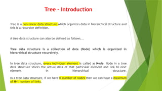
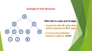
Tree – Introduction
Treeis a non-linear data structure which organizes data in hierarchical structure and
this is a recursive definition.
A tree data structure can also be defined as follows...
Tree data structure is a collection of data (Node) which is organized in
hierarchical structure recursively.
In tree data structure, every individual element is called as Node. Node in a tree
data structure stores the actual data of that particular element and link to next
element in hierarchical structure.
In a tree data structure, if we have N number of nodes then we can have a maximum
of N-1 number of links.
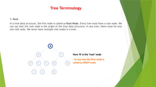
Tree Terminology
1. Root
Ina tree data structure, the first node is called as Root Node. Every tree must have a root node. We
can say that the root node is the origin of the tree data structure. In any tree, there must be only
one root node. We never have multiple root nodes in a tree.
5.
2. Edge
In atree data structure, the connecting link between any two nodes is called
as EDGE. In a tree with 'N' number of nodes there will be a maximum of 'N-1' number
of edges.
6.
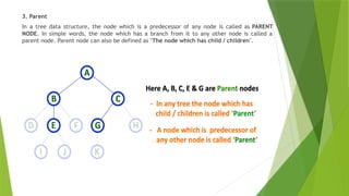
3. Parent
In atree data structure, the node which is a predecessor of any node is called as PARENT
NODE. In simple words, the node which has a branch from it to any other node is called a
parent node. Parent node can also be defined as "The node which has child / children".
7.
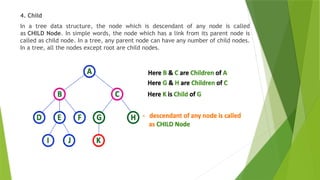
4. Child
In atree data structure, the node which is descendant of any node is called
as CHILD Node. In simple words, the node which has a link from its parent node is
called as child node. In a tree, any parent node can have any number of child nodes.
In a tree, all the nodes except root are child nodes.
8.
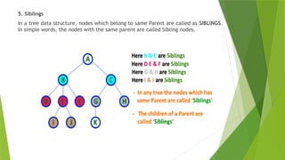
5. Siblings
In atree data structure, nodes which belong to same Parent are called as SIBLINGS.
In simple words, the nodes with the same parent are called Sibling nodes.
9.
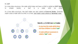
6. Leaf
In atree data structure, the node which does not have a child is called as LEAF Node.
In simple words, a leaf is a node with no child.
In a tree data structure, the leaf nodes are also called as External Nodes. External
node is also a node with no child. In a tree, leaf node is also called as 'Terminal' node.
10.
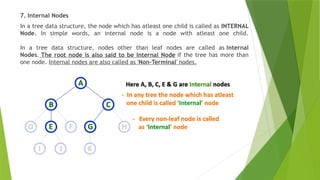
7. Internal Nodes
Ina tree data structure, the node which has atleast one child is called as INTERNAL
Node. In simple words, an internal node is a node with atleast one child.
In a tree data structure, nodes other than leaf nodes are called as Internal
Nodes. The root node is also said to be Internal Node if the tree has more than
one node. Internal nodes are also called as 'Non-Terminal' nodes.
11.
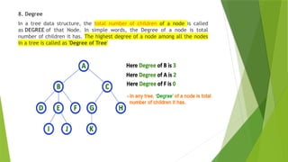
8. Degree
In atree data structure, the total number of children of a node is called
as DEGREE of that Node. In simple words, the Degree of a node is total
number of children it has. The highest degree of a node among all the nodes
in a tree is called as 'Degree of Tree'
12.
9. Level
In atree data structure, the root node is said to be at Level 0 and the children of
root node are at Level 1 and the children of the nodes which are at Level 1 will be
at Level 2 and so on... In simple words, in a tree each step from top to bottom is
called as a Level and the Level count starts with '0' and incremented by one at each
level (Step).
13.
10. Height
In atree data structure, the total number of edges from leaf node to a particular
node in the longest path is called as HEIGHT of that Node. In a tree, height of the
root node is said to be height of the tree. In a tree, height of all leaf nodes is '0'.
14.
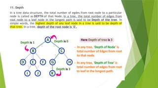
11. Depth
In atree data structure, the total number of egdes from root node to a particular
node is called as DEPTH of that Node. In a tree, the total number of edges from
root node to a leaf node in the longest path is said to be Depth of the tree. In
simple words, the highest depth of any leaf node in a tree is said to be depth of
that tree. In a tree, depth of the root node is '0'.
15.
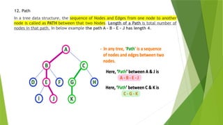
12. Path
In atree data structure, the sequence of Nodes and Edges from one node to another
node is called as PATH between that two Nodes. Length of a Path is total number of
nodes in that path. In below example the path A - B - E - J has length 4.
16.
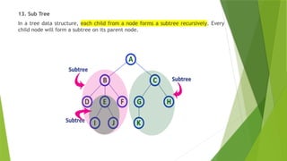
13. Sub Tree
Ina tree data structure, each child from a node forms a subtree recursively. Every
child node will form a subtree on its parent node.
17.
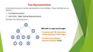
Tree Representations
A treedata structure can be represented in two methods. Those methods are as
follows...
List Representation
Left Child - Right Sibling Representation
Consider the following tree...
18.
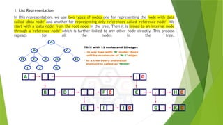
1. List Representation
Inthis representation, we use two types of nodes one for representing the node with data
called 'data node' and another for representing only references called 'reference node'. We
start with a 'data node' from the root node in the tree. Then it is linked to an internal node
through a 'reference node' which is further linked to any other node directly. This process
repeats for all the nodes in the tree.
19.
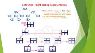
2. Left Child- Right Sibling Representation
In this representation, we use a list with one type of node which consists of three fields namely
Data field, Left child reference field and Right sibling reference field. Data field stores the actual
value of a node, left reference field stores the address of the left child and right reference field
stores the address of the right sibling node. Graphical representation of that node is as follows...
In this representation, every node's data field stores the actual value of that node. If
that node has left a child, then left reference field stores the address of that left child
node otherwise stores NULL. If that node has the right sibling, then right reference field
stores the address of right sibling node otherwise stores NULL.
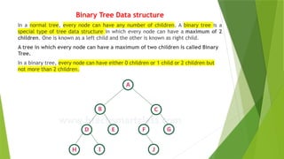
Binary Tree Datastructure
In a normal tree, every node can have any number of children. A binary tree is a
special type of tree data structure in which every node can have a maximum of 2
children. One is known as a left child and the other is known as right child.
A tree in which every node can have a maximum of two children is called Binary
Tree.
In a binary tree, every node can have either 0 children or 1 child or 2 children but
not more than 2 children.
22.
There are differenttypes of binary trees and they are...
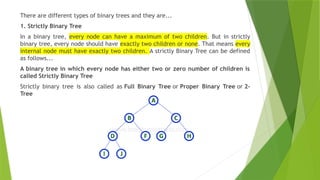
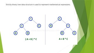
1. Strictly Binary Tree
In a binary tree, every node can have a maximum of two children. But in strictly
binary tree, every node should have exactly two children or none. That means every
internal node must have exactly two children. A strictly Binary Tree can be defined
as follows...
A binary tree in which every node has either two or zero number of children is
called Strictly Binary Tree
Strictly binary tree is also called as Full Binary Tree or Proper Binary Tree or 2-
Tree
23.
Strictly binary treedata structure is used to represent mathematical expressions.
24.
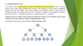
2. Complete BinaryTree
In a binary tree, every node can have a maximum of two children. But in strictly
binary tree, every node should have exactly two children or none and in complete
binary tree all the nodes must have exactly two children and at every level of
complete binary tree there must be 2level
number of nodes. For example at level 2
there must be 22
= 4 nodes and at level 3 there must be 23
= 8 nodes.
A binary tree in which every internal node has exactly two children and all leaf
nodes are at same level is called Complete Binary Tree.
Complete binary tree is also called as Perfect Binary Tree
25.
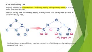
3. Extended BinaryTree
A binary tree can be converted into Full Binary tree by adding dummy nodes to existing
nodes wherever required.
The full binary tree obtained by adding dummy nodes to a binary tree is called as
Extended Binary Tree.
In above figure, a normal binary tree is converted into full binary tree by adding dummy
nodes (In pink colour).
26.
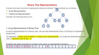
Binary Tree Representations
Abinary tree data structure is represented using two methods. Those methods are as follows...
Array Representation
Linked List Representation
Consider the following binary tree...
1. Array Representation of Binary Tree
In array representation of a binary tree, we use one-dimensional array (1-D Array) to represent a
binary tree.
To represent a binary tree of depth 'n' using array representation, we need one dimensional array
with a maximum size of 2n + 1.
Consider the above example of a binary tree and it is represented as follows...
27.
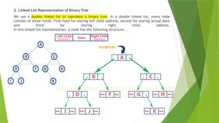
2. Linked ListRepresentation of Binary Tree
We use a double linked list to represent a binary tree. In a double linked list, every node
consists of three fields. First field for storing left child address, second for storing actual data
and third for storing right child address.
In this linked list representation, a node has the following structure...
28.
Binary Tree –ADT Algorithm
Procedure BinaryTree
//Objects : A finite set of nodes either empty or consisting of a root node, left
BinaryTree and rightBinaryTree
BinaryTree(); // Create an empty binary tree
Boolean IsEmpty(); // if the binary tree is empty, return TRUE(1); else return FALSE(0)
BinaryTree(BinaryTree bt1, Element <KeyType>item, BinaryTree bt2);
//Create a binary tree whose left subtree is bt1, whose right subtree is bt2 and whose
root node contains item
BinaryTree Lchild();
//if IsEmpty(), return error; else return the left subtree of *this
Element <keyType> Data();
//if IsEmpty(), return error; else return the data in the root node of *this
BinaryTree Rchild();
//if IsEmpty(), return error; else return the right subtree of *this
End Procedure
29.
Binary Tree Algorithm
Definition:A binary tree is a finite set of nodes which is either empty or consists of a root and two
disjoint binary trees called the left subtree and the right subtree.
structure BTREE
declare CREATE( ) → btree
ISEMTBT(btree) → boolean
MAKEBT(btree,item,btree) → btree
LCHILD(btree) → btree
DATA(btree) → item
RCHILD(btree) → btree
for all p,r btree, d item let
ISEMTBT(CREATE) :: = true
ISEMTBT(MAKEBT(p,d,r)) :: = false
LCHILD(MAKEBT(p,d,r)):: = p; LCHILD(CREATE):: = error
DATA(MAKEBT(p,d,r)) :: = d; DATA(CREATE) :: = error
RCHILD(MAKEBT(p,d,r)) :: = r; RCHILD(CREATE) :: = error
end
30.
Binary Tree Operations
Insertion
Deletion
Traversal
It Consists of three types
In-order Traversal (LC,ROOT,RC)
Pre-order Traversal (ROOT, LC,RC)
Post-order Traversal (LC,RC,ROOT)
31.
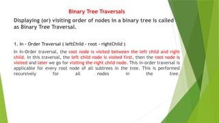
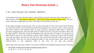
Binary Tree Traversals
Displaying(or) visiting order of nodes in a binary tree is called
as Binary Tree Traversal.
1. In - Order Traversal ( leftChild - root - rightChild )
In In-Order traversal, the root node is visited between the left child and right
child. In this traversal, the left child node is visited first, then the root node is
visited and later we go for visiting the right child node. This in-order traversal is
applicable for every root node of all subtrees in the tree. This is performed
recursively for all nodes in the tree.
32.
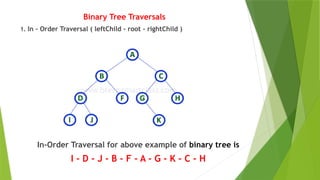
Binary Tree Traversals
1.In - Order Traversal ( leftChild - root - rightChild )
In-Order Traversal for above example of binary tree is
I - D - J - B - F - A - G - K - C - H
33.
Binary Tree Traversals
In- Order Traversal ( leftChild - root - rightChild )
procedure INORDER(T)
//T is a binary tree where each node has three fields
LCHILD,DATA,RCHILD//
if T = 0 then [call INORDER(LCHILD(T))
print(DATA(T))// Root
call(INORDER(RCHILD(T))]
end INORDER
34.
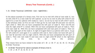
Binary Tree Traversals(Contd…)
1. In - Order Traversal ( leftChild - root - rightChild )
In the above example of a binary tree, first we try to visit left child of root node 'A', but
A's left child 'B' is a root node for left subtree. so we try to visit its (B's) left child 'D' and
again D is a root for subtree with nodes D, I and J. So we try to visit its left child 'I' and it
is the leftmost child. So first we visit 'I' then go for its root node 'D' and later we visit D's
right child 'J'. With this we have completed the left part of node B. Then visit 'B' and
next B's right child 'F' is visited. With this we have completed left part of node A. Then
visit root node 'A'. With this we have completed left and root parts of node A. Then we
go for the right part of the node A. In right of A again there is a subtree with root C. So go
for left child of C and again it is a subtree with root G. But G does not have left part so
we visit 'G' and then visit G's right child K. With this we have completed the left part of
node C. Then visit root node 'C' and next visit C's right child 'H' which is the rightmost
child in the tree. So we stop the process.
That means here we have visited in the order of I - D - J - B - F - A - G - K - C - H using
In-Order Traversal.
In-Order Traversal for above example of binary tree is
I - D - J - B - F - A - G - K - C - H
35.
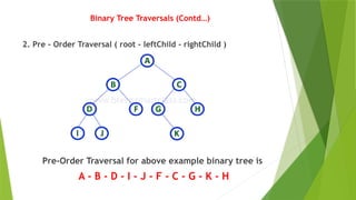
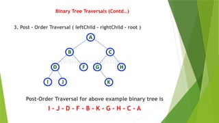
Binary Tree Traversals(Contd…)
2. Pre - Order Traversal ( root - leftChild - rightChild )
Pre-Order Traversal for above example binary tree is
A - B - D - I - J - F - C - G - K - H
36.
Binary Tree Traversals(Contd…)
Pre - Order Traversal ( root - leftChild - rightChild )
procedure PREORDER (T)
//T is a binary tree where each node has three fields
LCHILD,DATA,RCHILD//
if T = 0 then [print (DATA(T))
call PREORDER(LCHILD(T))
call PREORDER(RCHILD(T))]]
end PREORDER
37.
Binary Tree Traversals(Contd…)
2. Pre - Order Traversal ( root - leftChild - rightChild )
In Pre-Order traversal, the root node is visited before the left child and right child nodes. In
this traversal, the root node is visited first, then its left child and later its right child. This pre-
order traversal is applicable for every root node of all subtrees in the tree.
In the above example of binary tree, first we visit root node 'A' then visit its left child 'B' which
is a root for D and F. So we visit B's left child 'D' and again D is a root for I and J. So we visit D's
left child 'I' which is the leftmost child. So next we go for visiting D's right child 'J'. With this
we have completed root, left and right parts of node D and root, left parts of node B. Next visit
B's right child 'F'. With this we have completed root and left parts of node A. So we go for A's
right child 'C' which is a root node for G and H. After visiting C, we go for its left child 'G' which
is a root for node K. So next we visit left of G, but it does not have left child so we go for G's
right child 'K'. With this, we have completed node C's root and left parts. Next visit C's right
child 'H' which is the rightmost child in the tree. So we stop the process.
That means here we have visited in the order of A-B-D-I-J-F-C-G-K-H using Pre-Order Traversal.
Pre-Order Traversal for above example binary tree is
A - B - D - I - J - F - C - G - K - H
38.
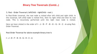
Binary Tree Traversals(Contd…)
3. Post - Order Traversal ( leftChild - rightChild - root )
Post-Order Traversal for above example binary tree is
I - J - D - F - B - K - G - H - C - A
39.
Binary Tree Traversals(Contd…)
Post - Order Traversal ( leftChild - rightChild - root )
procedure POSTORDER (T)
//T is a binary tree where each node has three fields L
CHILD,DATA,RCHILD//
if T = 0 then [call POSTORDER(LCHILD(T))
call POSTORDER(RCHILD(T))
print (DATA(T))]
end POSTORDER
40.
Binary Tree Traversals(Contd…)
3. Post - Order Traversal ( leftChild - rightChild - root )
In Post-Order traversal, the root node is visited after left child and right child. In
this traversal, left child node is visited first, then its right child and then its root
node. This is recursively performed until the right most node is visited.
Here we have visited in the order of I - J - D - F - B - K - G - H - C - A using Post-
Order Traversal.
Post-Order Traversal for above example binary tree is
I - J - D - F - B - K - G - H - C - A
41.
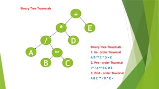
Binary Tree Traversals
+
*E
**
A
D
C
/
B
Binary Tree Traversals
1. In- order Traversal
A/B ** C * D + E
2. Pre – order Traversal
+* / A ** B C D E
3. Post – order Traversal
A B C ** / D * E +
42.
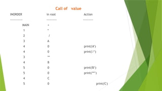
Call of value
INORDERin root Action
----------- --------- ---------
MAIN +
1 *
2 /
3 A
4 0 print('A’)
4 0 print('/’)
3 **
4 B
5 0 print('B’)
5 0 print('**’)
4 C
5 0 print('C')
43.
Call of value
INORDERin root Action
----------- --------- ---------
5 0 print('*’)
2 D
3 0 print('D’)
3 0 print('+’)
1 E
2 0 print('E’)
2 0
The elements get printed in the order
A/B ** C * D + E
44.
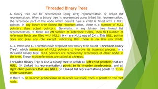
Threaded Binary Trees
Abinary tree can be represented using array representation or linked list
representation. When a binary tree is represented using linked list representation,
the reference part of the node which doesn't have a child is filled with a NULL
pointer. In any binary tree linked list representation, there is a number of NULL
pointers than actual pointers. Generally, in any binary tree linked list
representation, if there are 2N number of reference fields, then N+1 number of
reference fields are filled with NULL ( N+1 are NULL out of 2N ). This NULL pointer
does not play any role except indicating that there is no link (no child).
A. J. Perlis and C. Thornton have proposed new binary tree called "Threaded Binary
Tree", which makes use of NULL pointers to improve its traversal process. In a
threaded binary tree, NULL pointers are replaced by references of other nodes in
the tree. These extra references are called as threads.
Threaded Binary Tree is also a binary tree in which all left child pointers that are
NULL (in Linked list representation) points to its in-order predecessor, and all
right child pointers that are NULL (in Linked list representation) points to its in-
order successor.
If there is no in-order predecessor or in-order successor, then it points to the root
node.
45.
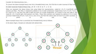
Consider the followingbinary tree...
To convert the above example binary tree into a threaded binary tree, first find the in-order traversal of that tree...
In-order traversal of above binary tree...H - D - I - B - E - A - F - J - C - G
When we represent the above binary tree using linked list representation, nodes H, I, E, F, J and G left child
pointers are NULL. This NULL is replaced by address of its in-order predecessor respectively (I to D, E to B, F to A, J
to F and G to C), but here the node H does not have its in-order predecessor, so it points to the root node A. And
nodes H, I, E, J and G right child pointers are NULL. These NULL pointers are replaced by address of its in-order
successor respectively (H to D, I to B, E to A, and J to C), but here the node G does not have its in-order successor, so
it points to the root node A.
Above example binary tree is converted into threaded binary tree as follows.
In the above figure, threads are indicated with dotted links.
46.
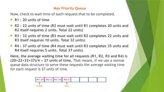
Max Priority Queue
Inthe normal queue data structure, insertion is performed at the end of the queue and
deletion is performed based on the FIFO principle. This queue implementation may not
be suitable for all applications.
Consider a networking application where the server has to respond for requests from
multiple clients using queue data structure. Assume four requests arrived at the queue
in the order of R1, R2, R3 & R4 where R1 requires 20 units of time, R2 requires 2 units
of time, R3 requires 10 units of time and R4 requires 5 units of time. A queue is as
follows...
47.
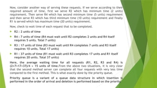
Max Priority Queue
Now,check to wait time of each request that to be completed.
R1 : 20 units of time
R2 : 22 units of time (R2 must wait until R1 completes 20 units and
R2 itself requires 2 units. Total 22 units)
R3 : 32 units of time (R3 must wait until R2 completes 22 units and
R3 itself requires 10 units. Total 32 units)
R4 : 37 units of time (R4 must wait until R3 completes 35 units and
R4 itself requires 5 units. Total 37 units)
Here, the average waiting time for all requests (R1, R2, R3 and R4) is
(20+22+32+37)/4 ≈ 27 units of time. That means, if we use a normal
queue data structure to serve these requests the average waiting time
for each request is 27 units of time.
48.
Now, consider anotherway of serving these requests. If we serve according to their
required amount of time, first we serve R2 which has minimum time (2 units)
requirement. Then serve R4 which has second minimum time (5 units) requirement
and then serve R3 which has third minimum time (10 units) requirement and finally
R1 is served which has maximum time (20 units) requirement.
Now, check to wait time of each request that to be completed.
R2 : 2 units of time
R4 : 7 units of time (R4 must wait until R2 completes 2 units and R4 itself
requires 5 units. Total 7 units)
R3 : 17 units of time (R3 must wait until R4 completes 7 units and R3 itself
requires 10 units. Total 17 units)
R1 : 37 units of time (R1 must wait until R3 completes 17 units and R1 itself
requires 20 units. Total 37 units)
Here, the average waiting time for all requests (R1, R2, R3 and R4) is
(2+7+17+37)/4 ≈ 15 units of time.From the above two situations, it is very clear
that the second method server can complete all four requests with very less time
compared to the first method. This is what exactly done by the priority queue.
Priority queue is a variant of a queue data structure in which insertion is
performed in the order of arrival and deletion is performed based on the priority.
49.
There are twotypes of priority queues they are as follows...
Max Priority Queue
Min Priority Queue
1. Max Priority Queue
In a max priority queue, elements are inserted in the order in which they arrive the
queue and the maximum value is always removed first from the queue. For example,
assume that we insert in the order 8, 3, 2 & 5 and they are removed in the order 8,
5, 3, 2.
The following are the operations performed in a Max priority queue...
isEmpty() - Check whether queue is Empty.
insert() - Inserts a new value into the queue.
findMax() - Find maximum value in the queue.
remove() - Delete maximum value from the queue.
50.
2. Min PriorityQueue Representations
Min Priority Queue is similar to max priority queue except for the removal of
maximum element first. We remove minimum element first in the min-priority
queue.
The following operations are performed in Min Priority Queue...
isEmpty() - Check whether queue is Empty.
insert() - Inserts a new value into the queue.
findMin() - Find minimum value in the queue.
remove() - Delete minimum value from the queue.
51.
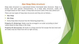
Max Heap Datastructure
Heap data structure is a specialized binary tree-based data structure. Heap is a
binary tree with special characteristics. In a heap data structure, nodes are
arranged based on their values. A heap data structure some times also called as B
There are two types of heap data structures and they are as follows...
Max Heap
Min Heap
Every heap data structure has the following properties...
Property #1 (Ordering): Nodes must be arranged in an order according to their
values based on Max heap or Min heap.
Property #2 (Structural): All levels in a heap must be full except the last level and
all nodes must be filled from left to right strictly.
52.
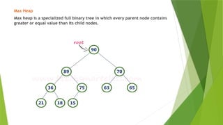
Max Heap
Max heapis a specialized full binary tree in which every parent node contains
greater or equal value than its child nodes.
53.
Operations on MaxHeap
The following operations are performed on a Max heap
data structure...
Finding Maximum
Insertion
Deletion
54.
Finding Maximum ValueOperation in Max Heap
Finding the node which has maximum value in a max heap is very simple. In
a max heap, the root node has the maximum value than all other nodes. So,
directly we can display root node value as the maximum value in max heap.
Insertion Operation in Max Heap
Insertion Operation in max heap is performed as follows...
Step 1 - Insert the newNode as last leaf from left to right.
Step 2 - Compare newNode value with its Parent node.
Step 3 - If newNode value is greater than its parent, then swap both of
them.
Step 4 - Repeat step 2 and step 3 until newNode value is less than its
parent node (or) newNode reaches to root.
55.
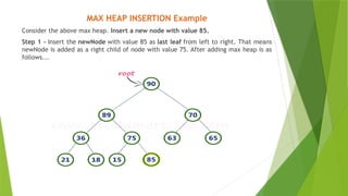
MAX HEAP INSERTIONExample
Consider the above max heap. Insert a new node with value 85.
Step 1 - Insert the newNode with value 85 as last leaf from left to right. That means
newNode is added as a right child of node with value 75. After adding max heap is as
follows...
56.
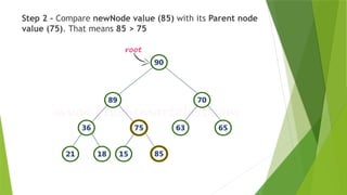
Step 2 -Compare newNode value (85) with its Parent node
value (75). That means 85 > 75
57.
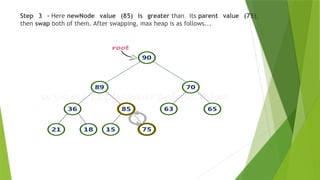
Step 3 -Here newNode value (85) is greater than its parent value (75),
then swap both of them. After swapping, max heap is as follows...
58.
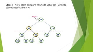
Step 4 -Now, again compare newNode value (85) with its
parent node value (89).
59.
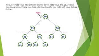
Here, newNode value(85) is smaller than its parent node value (89). So, we stop
insertion process. Finally, max heap after insertion of a new node with value 85 is as
follows...
60.
Deletion Operation inMax Heap
In a max heap, deleting the last node is very simple as it does not disturb max heap
properties.
Deleting root node from a max heap is little difficult as it disturbs the max heap
properties. We use the following steps to delete the root node from a max heap...
Step 1 - Swap the root node with last node in max heap
Step 2 - Delete last node.
Step 3 - Now, compare root value with its left child value.
Step 4 - If root value is smaller than its left child, then compare left child with
its right sibling. Else goto Step 6
Step 5 - If left child value is larger than its right sibling, then swap root with left
child otherwise swap root with its right child.
Step 6 - If root value is larger than its left child, then compare root value with
its right child value.
Step 7 - If root value is smaller than its right child, then swap root with right
child otherwise stop the process.
Step 8 - Repeat the same until root node fixes at its exact position.
61.
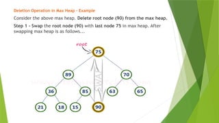
Deletion Operation inMax Heap – Example
Consider the above max heap. Delete root node (90) from the max heap.
Step 1 - Swap the root node (90) with last node 75 in max heap. After
swapping max heap is as follows...
62.
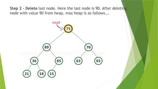
Step 2 -Delete last node. Here the last node is 90. After deleting
node with value 90 from heap, max heap is as follows...
63.
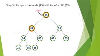
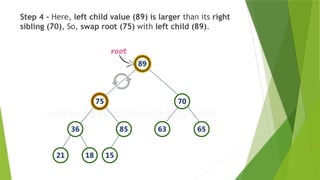
Step 3 -Compare root node (75) with its left child (89).
64.
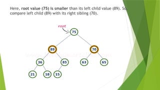
Here, root value(75) is smaller than its left child value (89). So,
compare left child (89) with its right sibling (70).
65.
Step 4 -Here, left child value (89) is larger than its right
sibling (70), So, swap root (75) with left child (89).
66.
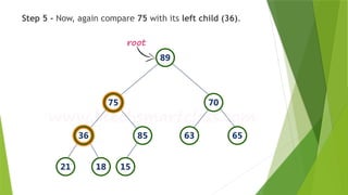
Step 5 -Now, again compare 75 with its left child (36).
67.
Here, node withvalue 75 is larger than its left child. So, we
compare node 75 with its right child 85.
68.
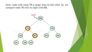
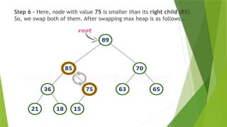
Step 6 -Here, node with value 75 is smaller than its right child (85).
So, we swap both of them. After swapping max heap is as follows...
69.
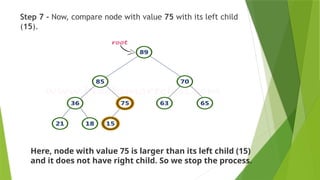
Step 7 -Now, compare node with value 75 with its left child
(15).
Here, node with value 75 is larger than its left child (15)
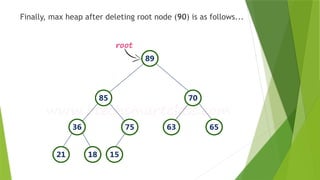
and it does not have right child. So we stop the process.
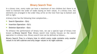
Binary Search Tree
Ina binary tree, every node can have a maximum of two children but there is no
need to maintain the order of nodes basing on their values. In a binary tree, the
elements are arranged in the order they arrive at the tree from top to bottom and
left to right.
A binary tree has the following time complexities...
Search Operation - O(n)
Insertion Operation - O(1)
Deletion Operation - O(n)
To enhance the performance of binary tree, we use a special type of binary tree
known as Binary Search Tree. Binary search tree mainly focuses on the search
operation in a binary tree. Binary search tree can be defined as follows...
Binary Search Tree is a binary tree in which every node contains only smaller
values in its left subtree and only larger values in its right subtree.
72.
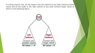
In a binarysearch tree, all the nodes in the left subtree of any node contains smaller
values and all the nodes in the right subtree of any node contains larger values as
shown in the following figure...
73.
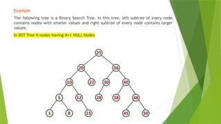
Example
The following treeis a Binary Search Tree. In this tree, left subtree of every node
contains nodes with smaller values and right subtree of every node contains larger
values.
In BST Tree N nodes having N+1 NULL Nodes
74.
Operations on aBinary Search Tree
The following operations are performed on a binary search tree...
Insertion
Search
Deletion
Every binary search tree is a binary tree but every binary tree need not to be
binary search tree.
A binary tree is a non-linear data structure in which a node can have utmost two
children, i.e., a node can have 0, 1 or maximum two children. A binary search
tree is an ordered binary tree in which some order is followed to organize the
nodes in a tree.
75.
Binary Search Algorithm
Whatis Search?
Search is a process of finding a value in a list of values. In other words, searching is the
process of locating given value position in a list of values.
Binary Search Algorithm
Binary search algorithm finds a given element in a list of elements with O(log n) time
complexity where n is total number of elements in the list. The binary search algorithm
can be used with only a sorted list of elements. That means the binary search is used
only with a list of elements that are already arranged in an order. The binary search can
not be used for a list of elements arranged in random order. This search process starts
comparing the search element with the middle element in the list. If both are matched,
then the result is "element found". Otherwise, we check whether the search element is
smaller or larger than the middle element in the list. If the search element is smaller,
then we repeat the same process for the left sublist of the middle element. If the search
element is larger, then we repeat the same process for the right sublist of the middle
element. We repeat this process until we find the search element in the list or until we
left with a sublist of only one element. And if that element also doesn't match with the
search element, then the result is "Element not found in the list".
76.
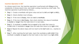
Insertion Operation inBST
In a binary search tree, the insertion operation is performed with O(log n) time
complexity. In binary search tree, new node is always inserted as a leaf node. The
insertion operation is performed as follows...
Step 1 - Create a newNode with given value and set its left and right to NULL.
Step 2 - Check whether tree is Empty.
Step 3 - If the tree is Empty, then set root to newNode.
Step 4 - If the tree is Not Empty, then check whether the value of newNode
is smaller or larger than the node (here it is root node).
Step 5 - If newNode is smaller than or equal to the node then move to
its left child. If newNode is larger than the node then move to its right child.
Step 6- Repeat the above steps until we reach to the leaf node (i.e., reaches to
NULL).
Step 7 - After reaching the leaf node, insert the newNode as left child if the
newNode is smaller or equal to that leaf node or else insert it as right child.
77.
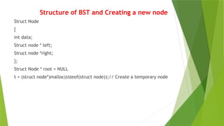
Structure of BSTand Creating a new node
Struct Node
{
int data;
Struct node * left;
Struct node *right;
};
Struct Node * root = NULL
t = (struct node*)malloc(sizeof(struct node));// Create a temporary node
78.
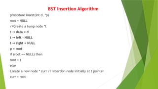
BST Insertion Algorithm
procedureinsert(int d, *p)
root = NULL
//Create a temp node *t
t data = d
→
t left – NULL
→
t right = NULL
→
p = root
if (root == NULL) then
root = t
else
Create a new node * curr // insertion node initially at t pointer
curr = root
79.
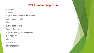
BST Insertion Algorithm
loop(curr)
p = curr
if ( t data > curr data) then
→ →
curr = curr right
→
else
curr = curr left
→
Repeat forever
if ( t data > p data) then
→ →
p right = t
→
else
p left = t
→
end procedure
80.
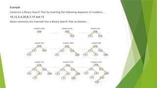
Example
Construct a BinarySearch Tree by inserting the following sequence of numbers...
10,12,5,4,20,8,7,15 and 13
Above elements are inserted into a Binary Search Tree as follows...
81.
Binary Search Algorithm
Procedurebinary_search
A = sorted array
N = size of array
X = value to be searched
Set lowerbound = 0
Set upperbound = n
loop x not found
If upperbound < lowerbound
EXIT : X does not exists.
Set midpoint = lowerbound + (upperbound – lowerbound) /2
If A[midpoint] < X then
Set lowerbound = midpoint + 1
midpoint = lowerbound + (upperbound – lowerbound) /2
If A[midpoint] > X then
Set upperbound = midpoint -1
midpoint = lowerbound + (upperbound – lowerbound) /2
If A[midpoint] = X then
EXIT: X found at location midpoint
End loop
End procedure
82.
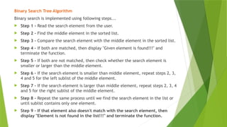
Binary Search TreeAlgorithm
Binary search is implemented using following steps...
Step 1 - Read the search element from the user.
Step 2 - Find the middle element in the sorted list.
Step 3 - Compare the search element with the middle element in the sorted list.
Step 4 - If both are matched, then display "Given element is found!!!" and
terminate the function.
Step 5 - If both are not matched, then check whether the search element is
smaller or larger than the middle element.
Step 6 - If the search element is smaller than middle element, repeat steps 2, 3,
4 and 5 for the left sublist of the middle element.
Step 7 - If the search element is larger than middle element, repeat steps 2, 3, 4
and 5 for the right sublist of the middle element.
Step 8 - Repeat the same process until we find the search element in the list or
until sublist contains only one element.
Step 9 - If that element also doesn't match with the search element, then
display "Element is not found in the list!!!" and terminate the function.
84.
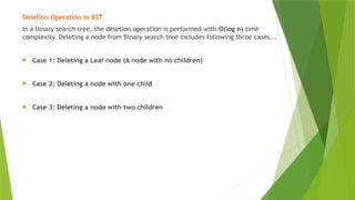
Deletion Operation inBST
In a binary search tree, the deletion operation is performed with O(log n) time
complexity. Deleting a node from Binary search tree includes following three cases...
Case 1: Deleting a Leaf node (A node with no children)
Case 2: Deleting a node with one child
Case 3: Deleting a node with two children
85.
Case 1: Deletinga leaf node
We use the following steps to delete a leaf node from BST...
Step 1 - Find the node to be deleted using search operation
Step 2 – Get the deleted value by using search operation and place it in the
current node
Step 3 - Delete the node using free function (If it is a leaf) and terminate the
function.
if (curr == parent right) then
→
parent right == NULL
→
else
parent left == NULL
→
free (curr)
86.
Case 2: Deletinga node with one child
We use the following steps to delete a node with one child from BST...
Step 1 - Find the node to be deleted using search operation
Step 2 - If it has only one child then create a link between its parent node and
child node in a four different ways
Step 3 - Get the deleted value by using search operation and place it in the
current node
Step 4 - Delete the node using free function and terminate the function.
87.
Case 2: Deletinga node with one child
Four Different Ways
First Way
if (curr left ! = NULL) then
→
if (curr == parent right)
→
parent right ==
→ curr left
→
curr left = NULL
→
free (curr)
Second Way
if (curr right ! = NULL) then
→
if (curr == parent right)
→
parent right ==
→ curr right
→
curr right = NULL
→
free (curr)
88.
Case 2: Deletinga node with one child
Four Different Ways
Third Way
if (curr right ! = NULL) then
→
if (curr == parent left)
→
parent left ==
→ curr right
→
curr right = NULL
→
free (curr)
Fourth Way
if (curr left ! = NULL) then
→
if (curr == parent left)
→
parent left ==
→ curr left
→
curr left = NULL
→
free (curr)
89.
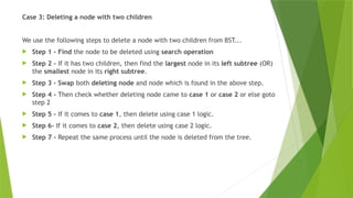
Case 3: Deletinga node with two children
We use the following steps to delete a node with two children from BST...
Step 1 - Find the node to be deleted using search operation
Step 2 - If it has two children, then find the largest node in its left subtree (OR)
the smallest node in its right subtree.
Step 3 - Swap both deleting node and node which is found in the above step.
Step 4 - Then check whether deleting node came to case 1 or case 2 or else goto
step 2
Step 5 - If it comes to case 1, then delete using case 1 logic.
Step 6- If it comes to case 2, then delete using case 2 logic.
Step 7 - Repeat the same process until the node is deleted from the tree.
90.
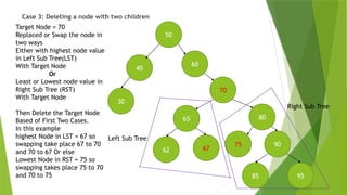
Case 3: Deletinga node with two children
90
50
40
60
30
62
70
67
80
65
95
75
85
Left Sub Tree
Right Sub Tree
Target Node = 70
Replaced or Swap the node in
two ways
Either with highest node value
in Left Sub Tree(LST)
With Target Node
Or
Least or Lowest node value in
Right Sub Tree (RST)
With Target Node
Then Delete the Target Node
Based of First Two Cases.
In this example
highest Node in LST = 67 so
swapping take place 67 to 70
and 70 to 67 Or else
Lowest Node in RST = 75 so
swapping takes place 75 to 70
and 70 to 75
91.
SET OPERATIONS
Union
Intersection
Difference
Cartesian Product
Complement
Null Set
Cardinality
Equivalence of Sets
Disjoint Sets
92.
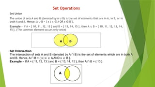
Set Operations
Set Union
Theunion of sets A and B (denoted by A B) is the set of elements that are in A, in B, or in
∪
both A and B. Hence, A B = { x | x A OR x B }.
∪ ∈ ∈
Example − If A = { 10, 11, 12, 13 } and B = { 13, 14, 15 }, then A B = { 10, 11, 12, 13, 14,
∪
15 }. (The common element occurs only once)
Set Intersection
The intersection of sets A and B (denoted by A ∩ B) is the set of elements which are in both A
and B. Hence, A ∩ B = { x | x A AND x B }.
∈ ∈
Example − If A = { 11, 12, 13 } and B = { 13, 14, 15 }, then A ∩ B = { 13 }.
93.
Set Operations
Set Difference/Relative Complement
The set difference of sets A and B (denoted by A – B) is the set of elements that are only in A but
not in B. Hence, A - B = { x | x A AND x B }.
∈ ∉
Example − If A = { 10, 11, 12, 13 } and B = { 13, 14, 15 }, then (A - B) = { 10, 11, 12 } and (B - A)
= { 14, 15 }. Here, we can see (A - B) ≠ (B - A)
Complement of a Set
The complement of a set A (denoted by A’) is the set of elements which are not in set A.
Hence, A' = { x | x A }.
∉
More specifically, A'= (U - A) where U is a universal set that contains all objects.
Example − If A = { x | x belongs to set of odd integers } then A' = { y | y does not belong to set
of odd integers }
94.
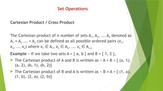
Set Operations
Cartesian Product/ Cross Product
The Cartesian product of n number of sets A1, A2, ... An denoted as
A1 × A2 ... × An can be defined as all possible ordered pairs (x1,
x2, ... xn) where x1 A
∈ 1, x2 A
∈ 2, ... xn A_
∈ n
Example − If we take two sets A = { a, b } and B = { 1, 2 },
The Cartesian product of A and B is written as − A × B = { (a, 1),
(a, 2), (b, 1), (b, 2)}
The Cartesian product of B and A is written as − B × A = { (1, a),
(1, b), (2, a), (2, b)}
95.
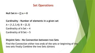
Set Operations
Null SetA = {} a = 0
Cardinality – Number of elements in a given set
A = {1,2,3,4}; B = {2,3}
Cardinality of A Set = 4
Cardinality of B Set = 5
Disjoint Sets – No Connection between two Sets
Find the Connection either two ends of the sets or beginning of the
two sets finally Combine the two Sets (Union)
96.
Set Operations inData Structures
List Representation
Hash Table Representation
Bit Vector
Tree Representation
97.
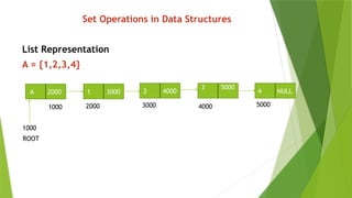
Set Operations inData Structures
List Representation
A = {1,2,3,4}
A 2000 1 3000 4 NULL
3 5000
2 4000
1000 2000 3000 4000 5000
1000
ROOT
98.
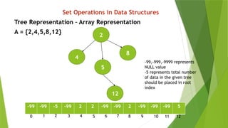
Set Operations inData Structures
Tree Representation – Array Representation
A = {2,4,5,8,12}
2
12
4
5
8
-99 -99 -5 -99 2 2 -99 -99 2 -99 -99 -99 5
-99,-999,-9999 represents
NULL value
-5 represents total number
of data in the given tree
should be placed in root
index
0 2
1 3 4 5 7
6 8 9 10 11 12


![Binary Tree Traversals
In - Order Traversal ( leftChild - root - rightChild )
procedure INORDER(T)
//T is a binary tree where each node has three fields
LCHILD,DATA,RCHILD//
if T = 0 then [call INORDER(LCHILD(T))
print(DATA(T))// Root
call(INORDER(RCHILD(T))]
end INORDER](https://image.slidesharecdn.com/ds-chapter5-260118064644-b52ed6e3/85/Data-Structure-Tree-and-Binary-Tree-Structure-33-320.jpg)
![Binary Tree Traversals (Contd…)
Pre - Order Traversal ( root - leftChild - rightChild )
procedure PREORDER (T)
//T is a binary tree where each node has three fields
LCHILD,DATA,RCHILD//
if T = 0 then [print (DATA(T))
call PREORDER(LCHILD(T))
call PREORDER(RCHILD(T))]]
end PREORDER](https://image.slidesharecdn.com/ds-chapter5-260118064644-b52ed6e3/85/Data-Structure-Tree-and-Binary-Tree-Structure-36-320.jpg)
![Binary Tree Traversals (Contd…)
Post - Order Traversal ( leftChild - rightChild - root )
procedure POSTORDER (T)
//T is a binary tree where each node has three fields L
CHILD,DATA,RCHILD//
if T = 0 then [call POSTORDER(LCHILD(T))
call POSTORDER(RCHILD(T))
print (DATA(T))]
end POSTORDER](https://image.slidesharecdn.com/ds-chapter5-260118064644-b52ed6e3/85/Data-Structure-Tree-and-Binary-Tree-Structure-39-320.jpg)


![Binary Search Algorithm
Procedure binary_search
A = sorted array
N = size of array
X = value to be searched
Set lowerbound = 0
Set upperbound = n
loop x not found
If upperbound < lowerbound
EXIT : X does not exists.
Set midpoint = lowerbound + (upperbound – lowerbound) /2
If A[midpoint] < X then
Set lowerbound = midpoint + 1
midpoint = lowerbound + (upperbound – lowerbound) /2
If A[midpoint] > X then
Set upperbound = midpoint -1
midpoint = lowerbound + (upperbound – lowerbound) /2
If A[midpoint] = X then
EXIT: X found at location midpoint
End loop
End procedure](https://image.slidesharecdn.com/ds-chapter5-260118064644-b52ed6e3/85/Data-Structure-Tree-and-Binary-Tree-Structure-81-320.jpg)