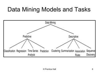
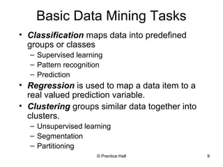
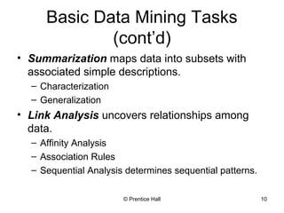
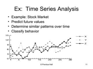
This document provides an overview and introduction to the course CIS 674 Introduction to Data Mining. It defines data mining, outlines basic data mining tasks such as classification, clustering, and association rule mining. It also discusses the relationship between data mining and knowledge discovery in databases (KDD), and highlights some issues in data mining such as handling large datasets, high dimensionality, and interpretation of results.

1. CIS 674
Introduction to Data Mining
Srinivasan Parthasarathy
srini@cse.ohio-state.edu
Office Hours: TTH 2-3:18PM
DL317
© Prentice Hall 1

2. Introduction Outline
GGooaall:: PPrroovviiddee aann oovveerrvviieeww ooff ddaattaa mmiinniinngg..
• Define data mining
• Data mining vs. databases
• Basic data mining tasks
• Data mining development
• Data mining issues
© Prentice Hall 2

3. Introduction
• Data is produced at a phenomenal rate
• Our ability to store has grown
• Users expect more sophisticated
information
• How?
UUNNCCOOVVEERR HHIIDDDDEENN IINNFFOORRMMAATTIIOONN
DDAATTAA MMIINNIINNGG
© Prentice Hall 3

4. Data Mining
• Objective: Fit data to a model
• Potential Result: Higher-level meta
information that may not be obvious when
looking at raw data
• Similar terms
– Exploratory data analysis
– Data driven discovery
– Deductive learning
© Prentice Hall 4

5. Data Mining Algorithm
• Objective: Fit Data to a Model
– Descriptive
– Predictive
• Preferential Questions
– Which technique to choose?
• ARM/Classification/Clustering
• Answer: Depends on what you want to do with data?
– Search Strategy – Technique to search the data
• Interface? Query Language?
• Efficiency
© Prentice Hall 5

6. Database Processing vs. Data
Mining Processing
© Prentice Hall 6
• Query
– Well defined
– SQL
• Query
– Poorly defined
– No precise query language
 OOuuttppuutt
– PPrreecciissee
– SSuubbsseett ooff ddaattaabbaassee
 OOuuttppuutt
– FFuuzzzzyy
– NNoott aa ssuubbsseett ooff ddaattaabbaassee

7. Query Examples
– FFiinndd aallll ccrreeddiitt aapppplliiccaannttss wwiitthh llaasstt nnaammee ooff SSmmiitthh..
– IIddeennttiiffyy ccuussttoommeerrss wwhhoo hhaavvee ppuurrcchhaasseedd mmoorree
tthhaann $$1100,,000000 iinn tthhee llaasstt mmoonntthh..
– Find all customers who hhaavvee ppuurrcchhaasseedd mmiillkk
– FFiinndd aallll ccrreeddiitt aapppplliiccaannttss wwhhoo aarree ppoooorr ccrreeddiitt
rriisskkss.. ((ccllaassssiiffiiccaattiioonn))
– IIddeennttiiffyy ccuussttoommeerrss wwiitthh ssiimmiillaarr bbuuyyiinngg hhaabbiittss..
((CClluusstteerriinngg))
© Prentice Hall 7
• Database
• Data Mining
– FFiinndd aallll iitteemmss wwhhiicchh aarree ffrreeqquueennttllyy ppuurrcchhaasseedd
wwiitthh mmiillkk.. ((aassssoocciiaattiioonn rruulleess))

8. Data Mining Models and Tasks
© Prentice Hall 8

9. Basic Data Mining Tasks
• Classification maps data into predefined
groups or classes
– Supervised learning
– Pattern recognition
– Prediction
• Regression is used to map a data item to a
real valued prediction variable.
• Clustering groups similar data together into
clusters.
– Unsupervised learning
– Segmentation
– Partitioning
© Prentice Hall 9

10. Basic Data Mining Tasks
(cont’d)
• Summarization maps data into subsets with
associated simple descriptions.
– Characterization
– Generalization
• Link Analysis uncovers relationships among
data.
– Affinity Analysis
– Association Rules
– Sequential Analysis determines sequential patterns.
© Prentice Hall 10

11. Ex: Time Series Analysis
• Example: Stock Market
• Predict future values
• Determine similar patterns over time
• Classify behavior
© Prentice Hall 11

12. Data Mining vs. KDD
• Knowledge Discovery in Databases
(KDD): process of finding useful
information and patterns in data.
• Data Mining: Use of algorithms to extract
the information and patterns derived by
the KDD process.
© Prentice Hall 12

13. Knowledge Discovery Process
– Data mining: the core
of knowledge discovery
Knowledge Interpretation
process.
Data Mining
Task-relevant Data
Data transformations
Preprocessed
Data
Data Cleaning
Data Integration
Databases
Selection

14. KDD Process Ex: Web Log
• Selection:
– Select log data (dates and locations) to use
© Prentice Hall 14
• Preprocessing:
– Remove identifying URLs
– Remove error logs
• Transformation:
– Sessionize (sort and group)
• Data Mining:
– Identify and count patterns
– Construct data structure
• Interpretation/Evaluation:
– Identify and display frequently accessed sequences.
• Potential User Applications:
– Cache prediction
– Personalization

15. Data Mining Development
•Similarity Measures
•Hierarchical Clustering
•IR Systems
•Imprecise Queries
•Textual Data
•Web Search Engines
•Bayes Theorem
•Regression Analysis
•EM Algorithm
•K-Means Clustering
•Time Series Analysis
•Neural Networks
•Decision Tree Algorithms
DATA MINING
© Prentice Hall 15
•Relational Data Model
•SQL
•Association Rule Algorithms
•Data Warehousing
•Scalability Techniques
•Algorithm Design Techniques
•Algorithm Analysis
•Data Structures
HIGH PERFORMANCE

16. KDD Issues
• Human Interaction
• Overfitting
• Outliers
• Interpretation
• Visualization
• Large Datasets
• High Dimensionality
© Prentice Hall 16

17. KDD Issues (cont’d)
• Multimedia Data
• Missing Data
• Irrelevant Data
• Noisy Data
• Changing Data
• Integration
• Application
© Prentice Hall 17

18. Social Implications of DM
• Privacy
• Profiling
• Unauthorized use
© Prentice Hall 18

19. Data Mining Metrics
• Usefulness
• Return on Investment (ROI)
• Accuracy
• Space/Time
© Prentice Hall 19

20. Database Perspective on Data
Mining
• Scalability
• Real World Data
• Updates
• Ease of Use
© Prentice Hall 20

21. Outline of Today’s Class
• Statistical Basics
– Point Estimation
– Models Based on Summarization
– Bayes Theorem
– Hypothesis Testing
– Regression and Correlation
• Similarity Measures
© Prentice Hall 21

22. Point Estimation
• Point Estimate: estimate a population
parameter.
• May be made by calculating the parameter for a
sample.
• May be used to predict value for missing data.
• Ex:
– R contains 100 employees
– 99 have salary information
– Mean salary of these is $50,000
– Use $50,000 as value of remaining employee’s
salary.
Is this a good idea?
© Prentice Hall 22

23. Estimation Error
• Bias: Difference between expected value and
actual value.
• Mean Squared Error (MSE): expected value of
the squared difference between the estimate
and the actual value:
• Why square?
• Root Mean Square Error (RMSE)
© Prentice Hall 23

24. Jackknife Estimate
• Jackknife Estimate: estimate of parameter is
obtained by omitting one value from the set of
observed values.
– Treat the data like a population
– Take samples from this population
– Use these samples to estimate the parameter
• Let θ(hat) be an estimate on the entire pop.
• Let θ(j)(hat) be an estimator of the same form
with observation j deleted
• Allows you to examine the impact of outliers!
© Prentice Hall 24

25. Maximum Likelihood
Estimate (MLE)
• Obtain parameter estimates that maximize
the probability that the sample data occurs for
the specific model.
• Joint probability for observing the sample
data by multiplying the individual probabilities.
Likelihood function:
© Prentice Hall 25
• Maximize L.

26. MLE Example
• Coin toss five times: {H,H,H,H,T}
• Assuming a perfect coin with H and T equally
likely, the likelihood of this sequence is:
• However if the probability of a H is 0.8 then:
© Prentice Hall 26

27. MLE Example (cont’d)
• General likelihood formula:
• Estimate for p is then 4/5 = 0.8
© Prentice Hall 27

28. Expectation-Maximization (EM)
• Solves estimation with incomplete data.
• Obtain initial estimates for parameters.
• Iteratively use estimates for missing data
and continue until convergence.
© Prentice Hall 28

29. EM Example
© Prentice Hall 29

30. EM Algorithm
© Prentice Hall 30

31. Bayes Theorem Example
• Credit authorizations (hypotheses):
h1=authorize purchase, h2 = authorize after
further identification, h3=do not authorize,
h4= do not authorize but contact police
• Assign twelve data values for all
combinations of credit and income:
1 2 3 4
Excellent x1 x2 x3 x4
Good x5 x6 x7 x8
Bad x9 x10 x11 x12
• From training data: P(h1) = 60%; P(h2)=20%;
P(h3)=10%; P(h4)=10%.
© Prentice Hall 31

32. Bayes Example(cont’d)
© Prentice Hall 32
• Training Data:
ID Income Credit Class xi
1 4 Excellent h1 x4
2 3 Good h1 x7
3 2 Excellent h1 x2
4 3 Good h1 x7
5 4 Good h1 x8
6 2 Excellent h1 x2
7 3 Bad h2 x11
8 2 Bad h2 x10
9 3 Bad h3 x11
10 1 Bad h4 x9

33. Bayes Example(cont’d)
• Calculate P(xi|hj) and P(xi)
• Ex: P(x7|h1)=2/6; P(x4|h1)=1/6; P(x2|h1)=2/6; P(x8|
h1)=1/6; P(xi|h1)=0 for all other xi.
• Predict the class for x4:
– Calculate P(hj|x4) for all hj.
– Place x4 in class with largest value.
– Ex:
• P(h1|x4)=(P(x4|h1)(P(h1))/P(x4)
=(1/6)(0.6)/0.1=1.
© Prentice Hall 33
• x4 in class h1.

34. Other Statistical Measures
© Prentice Hall 34
• Chi-Squared
– O – observed value
– E – Expected value based on hypothesis.
• Jackknife Estimate
– estimate of parameter is obtained by omitting one value from the
set of observed values.
• Regression
– Predict future values based on past values
– Linear Regression assumes linear relationship exists.
y = c0 + c1 x1 + … + cn xn
• Find values to best fit the data
• Correlation

35. Similarity Measures
• Determine similarity between two objects.
• Similarity characteristics:
• Alternatively, distance measure measure how
unlike or dissimilar objects are.
© Prentice Hall 35

36. Similarity Measures
© Prentice Hall 36

37. Distance Measures
• Measure dissimilarity between objects
© Prentice Hall 37

38. Information Retrieval
• Information Retrieval (IR): retrieving desired
information from textual data.
• Library Science
• Digital Libraries
• Web Search Engines
• Traditionally keyword based
• Sample query:
Find all documents about “data mining”.
DM: Similarity measures;
Mine text/Web data.
© Prentice Hall 38

39. Information Retrieval (cont’d)
• Similarity: measure of how close a
query is to a document.
• Documents which are “close enough”
are retrieved.
• Metrics:
–Precision = |Relevant and Retrieved|
|Retrieved|
–Recall = |Relevant and Retrieved|
|Relevant|
© Prentice Hall 39

40. IR Query Result Measures and
Classification
IR Classification
© Prentice Hall 40