Data base management system - Parallel Database

Database System Concepts, 6th
Ed.
©Silberschatz, Korth and Sudarshan
See www.db-book.com for conditions on re-use
Chapter 18: Parallel Databases

18.2
Database System Concepts - 6th
Edition
 Introduction
 I/O Parallelism
 Interquery Parallelism
 Intraquery Parallelism
 Intraoperation Parallelism
 Interoperation Parallelism
 Design of Parallel Systems

18.3
Edition
Introduction
Introduction
 Parallel machines are becoming quite common and affordable
 Prices of microprocessors, memory and disks have dropped
sharply
 Recent desktop computers feature multiple processors and this
trend is projected to accelerate
 Databases are growing increasingly large
 large volumes of transaction data are collected and stored for later
analysis.
 multimedia objects like images are increasingly stored in
databases
 Large-scale parallel database systems increasingly used for:
 storing large volumes of data
 processing time-consuming decision-support queries
 providing high throughput for transaction processing

18.4
Edition
Parallelism in Databases
Parallelism in Databases
 Data can be partitioned across multiple disks for parallel I/O.
 Individual relational operations (e.g., sort, join, aggregation) can be
executed in parallel
 data can be partitioned and each processor can work
independently on its own partition.
 Queries are expressed in high level language (SQL, translated to
relational algebra)
 makes parallelization easier.
 Different queries can be run in parallel with each other.
Concurrency control takes care of conflicts.
 Thus, databases naturally lend themselves to parallelism.

18.5
Edition
I/O Parallelism
I/O Parallelism
 Reduce the time required to retrieve relations from disk by partitioning
 The relations on multiple disks.
 Horizontal partitioning – tuples of a relation are divided among many
disks such that each tuple resides on one disk.
 Partitioning techniques (number of disks = n):
Round-robin:
Send the I th
tuple inserted in the relation to disk i mod n.
Hash partitioning:
 Choose one or more attributes as the partitioning attributes.
 Choose hash function h with range 0…n - 1
 Let i denote result of hash function h applied to the
partitioning attribute value of a tuple. Send tuple to disk i.

18.6
Edition
I/O Parallelism (Cont.)
I/O Parallelism (Cont.)
 Partitioning techniques (cont.):
 Range partitioning:
 Choose an attribute as the partitioning attribute.
 A partitioning vector [vo, v1, ..., vn-2] is chosen.
 Let v be the partitioning attribute value of a tuple. Tuples such that
vi  vi+1 go to disk I + 1. Tuples with v < v0 go to disk 0 and tuples
with v  vn-2 go to disk n-1.
E.g., with a partitioning vector [5,11], a tuple with partitioning
attribute value of 2 will go to disk 0, a tuple with value 8 will go to
disk 1, while a tuple with value 20 will go to disk2.

18.7
Edition
Comparison of Partitioning Techniques
Comparison of Partitioning Techniques
 Evaluate how well partitioning techniques support the following types
of data access:
1. Scanning the entire relation.
2. Locating a tuple associatively – point queries.
 E.g., r.A = 25.
3. Locating all tuples such that the value of a given attribute lies within
a specified range – range queries.
 E.g., 10  r.A < 25.

18.8
Edition
Comparison of Partitioning Techniques (Cont.)
Round robin:
 Advantages
 Best suited for sequential scan of entire relation on each query.
 All disks have almost an equal number of tuples; retrieval work is
thus well balanced between disks.
 Range queries are difficult to process
 No clustering -- tuples are scattered across all disks

18.9
Edition
Hash partitioning:
 Good for sequential access
 Assuming hash function is good, and partitioning attributes form a
key, tuples will be equally distributed between disks
 Retrieval work is then well balanced between disks.
 Good for point queries on partitioning attribute
 Can lookup single disk, leaving others available for answering
other queries.
 Index on partitioning attribute can be local to disk, making lookup
and update more efficient
 No clustering, so difficult to answer range queries

18.10
Edition
 Range partitioning:
 Provides data clustering by partitioning attribute value.
 Good for sequential access
 Good for point queries on partitioning attribute: only one disk needs to
be accessed.
 For range queries on partitioning attribute, one to a few disks may need
to be accessed
 Remaining disks are available for other queries.
 Good if result tuples are from one to a few blocks.
 If many blocks are to be fetched, they are still fetched from one to a
few disks, and potential parallelism in disk access is wasted
 Example of execution skew.

18.11
Edition
Partitioning a Relation across Disks
Partitioning a Relation across Disks
 If a relation contains only a few tuples which will fit into a single disk
block, then assign the relation to a single disk.
 Large relations are preferably partitioned across all the available disks.
 If a relation consists of m disk blocks and there are n disks available in
the system, then the relation should be allocated min(m,n) disks.

18.12
Edition
Handling of Skew
Handling of Skew
 The distribution of tuples to disks may be skewed — that is, some
disks have many tuples, while others may have fewer tuples.
 Types of skew:
 Attribute-value skew.
 Some values appear in the partitioning attributes of many
tuples; all the tuples with the same value for the partitioning
attribute end up in the same partition.
 Can occur with range-partitioning and hash-partitioning.
 Partition skew.
 With range-partitioning, badly chosen partition vector may
assign too many tuples to some partitions and too few to
others.
 Less likely with hash-partitioning if a good hash-function is
chosen.

18.13
Edition
Handling Skew in Range-Partitioning
Handling Skew in Range-Partitioning
 To create a balanced partitioning vector (assuming partitioning
attribute forms a key of the relation):
 Sort the relation on the partitioning attribute.
 Construct the partition vector by scanning the relation in sorted
order as follows.
 After every 1/nth
of the relation has been read, the value of
the partitioning attribute of the next tuple is added to the
partition vector.
 n denotes the number of partitions to be constructed.
 Duplicate entries or imbalances can result if duplicates are
present in partitioning attributes.
 Alternative technique based on histograms used in practice

18.14
Edition
Handling Skew using Histograms
Handling Skew using Histograms
 Balanced partitioning vector can be constructed from histogram in a
relatively straightforward fashion
 Assume uniform distribution within each range of the histogram
 Histogram can be constructed by scanning relation, or sampling (blocks
containing) tuples of the relation

18.15
Edition
Handling Skew Using Virtual Processor
Handling Skew Using Virtual Processor
Partitioning
Partitioning
 Skew in range partitioning can be handled elegantly using virtual
processor partitioning:
 create a large number of partitions (say 10 to 20 times the number
of processors)
 Assign virtual processors to partitions either in round-robin fashion
or based on estimated cost of processing each virtual partition
 Basic idea:
 If any normal partition would have been skewed, it is very likely the
skew is spread over a number of virtual partitions
 Skewed virtual partitions get spread across a number of
processors, so work gets distributed evenly!

18.16
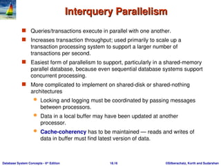
Edition
Interquery Parallelism
Interquery Parallelism
 Queries/transactions execute in parallel with one another.
 Increases transaction throughput; used primarily to scale up a
transaction processing system to support a larger number of
transactions per second.
 Easiest form of parallelism to support, particularly in a shared-memory
parallel database, because even sequential database systems support
concurrent processing.
 More complicated to implement on shared-disk or shared-nothing
architectures
 Locking and logging must be coordinated by passing messages
between processors.
 Data in a local buffer may have been updated at another
processor.
 Cache-coherency has to be maintained — reads and writes of
data in buffer must find latest version of data.

18.17
Edition
Cache Coherency Protocol
Cache Coherency Protocol
 Example of a cache coherency protocol for shared disk systems:
 Before reading/writing to a page, the page must be locked in
shared/exclusive mode.
 On locking a page, the page must be read from disk
 Before unlocking a page, the page must be written to disk if it
was modified.
 More complex protocols with fewer disk reads/writes exist.
 Cache coherency protocols for shared-nothing systems are similar.
Each database page is assigned a home processor. Requests to
fetch the page or write it to disk are sent to the home processor.

18.18
Edition
Intraquery Parallelism
Intraquery Parallelism
 Execution of a single query in parallel on multiple processors/disks;
important for speeding up long-running queries.
 Two complementary forms of intraquery parallelism:
 Intraoperation Parallelism – parallelize the execution of each
individual operation in the query.
 Interoperation Parallelism – execute the different operations in
a query expression in parallel.
the first form scales better with increasing parallelism because
the number of tuples processed by each operation is typically more
than the number of operations in a query.

18.19
Edition
Parallel Processing of Relational Operations
Parallel Processing of Relational Operations
 Our discussion of parallel algorithms assumes:
 read-only queries
 shared-nothing architecture
 n processors, P0, ..., Pn-1, and n disks D0, ..., Dn-1, where disk Di is
associated with processor Pi.
 If a processor has multiple disks they can simply simulate a single disk
Di.
 Shared-nothing architectures can be efficiently simulated on shared-
memory and shared-disk systems.
 Algorithms for shared-nothing systems can thus be run on shared-
memory and shared-disk systems.
 However, some optimizations may be possible.

18.20
Edition
Parallel Sort
Parallel Sort
Range-Partitioning Sort
 Choose processors P0, ..., Pm, where m  n -1 to do sorting.
 Create range-partition vector with m entries, on the sorting attributes
 Redistribute the relation using range partitioning
 all tuples that lie in the ith
range are sent to processor Pi
 Pi stores the tuples it received temporarily on disk Di.
 This step requires I/O and communication overhead.
 Each processor Pi sorts its partition of the relation locally.
 Each processors executes same operation (sort) in parallel with other
processors, without any interaction with the others (data parallelism).
 Final merge operation is trivial: range-partitioning ensures that, for 1 j
m, the key values in processor Pi
are all less than the key values in
Pj.

18.21
Edition
Parallel Sort (Cont.)
Parallel Sort (Cont.)
Parallel External Sort-Merge
 Assume the relation has already been partitioned among disks D0, ...,
Dn-1 (in whatever manner).
 Each processor Pi locally sorts the data on disk Di.
 The sorted runs on each processor are then merged to get the final
sorted output.
 Parallelize the merging of sorted runs as follows:
 The sorted partitions at each processor Pi are range-partitioned
across the processors P0, ..., Pm-1.
 Each processor Pi performs a merge on the streams as they are
received, to get a single sorted run.
 The sorted runs on processors P0,..., Pm-1 are concatenated to get
the final result.

18.22
Edition
Parallel Join
Parallel Join
 The join operation requires pairs of tuples to be tested to see if they
satisfy the join condition, and if they do, the pair is added to the join
output.
 Parallel join algorithms attempt to split the pairs to be tested over
several processors. Each processor then computes part of the join
locally.
 In a final step, the results from each processor can be collected
together to produce the final result.

18.23
Edition
Partitioned Join
Partitioned Join
 For equi-joins and natural joins, it is possible to partition the two input
relations across the processors, and compute the join locally at each
processor.
 Let r and s be the input relations, and we want to compute r r.A=s.B s.
 r and s each are partitioned into n partitions, denoted r0, r1, ..., rn-1 and
s0, s1, ..., sn-1.
 Can use either range partitioning or hash partitioning.
 r and s must be partitioned on their join attributes r.A and s.B), using
the same range-partitioning vector or hash function.
 Partitions ri and si are sent to processor Pi,
 Each processor Pi locally computes ri ri.A=si.B si. Any of the standard
join methods can be used.

18.24
Edition
Partitioned Join (Cont.)
Partitioned Join (Cont.)

18.25
Edition
Fragment-and-Replicate Join
Fragment-and-Replicate Join
 Partitioning not possible for some join conditions
 E.g., non-equijoin conditions, such as r.A > s.B.
 For joins were partitioning is not applicable, parallelization can be
accomplished by fragment and replicate technique
 Depicted on next slide
 Special case – asymmetric fragment-and-replicate:
 One of the relations, say r, is partitioned; any partitioning
technique can be used.
 The other relation, s, is replicated across all the processors.
 Processor Pi then locally computes the join of ri with all of s using
any join technique.

18.26
Edition
Depiction of Fragment-and-Replicate Joins
Depiction of Fragment-and-Replicate Joins

18.27
Edition
Fragment-and-Replicate Join (Cont.)
 General case: reduces the sizes of the relations at each processor.
 r is partitioned into n partitions,r0, r1, ..., r n-1;s is partitioned into m
partitions, s0, s1, ..., sm-1.
 Any partitioning technique may be used.
 There must be at least m * n processors.
 Label the processors as
 P0,0, P0,1, ..., P0,m-1, P1,0, ..., Pn-1m-1.
 Pi,j computes the join of ri with sj. In order to do so, ri is replicated
to Pi,0, Pi,1, ..., Pi,m-1, while si is replicated to P0,i, P1,i, ..., Pn-1,i
 Any join technique can be used at each processor Pi,j.

18.28
Edition
 Both versions of fragment-and-replicate work with any join condition,
since every tuple in r can be tested with every tuple in s.
 Usually has a higher cost than partitioning, since one of the relations
(for asymmetric fragment-and-replicate) or both relations (for general
fragment-and-replicate) have to be replicated.
 Sometimes asymmetric fragment-and-replicate is preferable even
though partitioning could be used.
 E.g., say s is small and r is large, and already partitioned. It may
be cheaper to replicate s across all processors, rather than
repartition r and s on the join attributes.

18.29
Edition
Partitioned Parallel Hash-Join
Partitioned Parallel Hash-Join
Parallelizing partitioned hash join:
 Assume s is smaller than r and therefore s is chosen as the build
relation.
 A hash function h1 takes the join attribute value of each tuple in s and
maps this tuple to one of the n processors.
 Each processor Pi reads the tuples of s that are on its disk Di, and
sends each tuple to the appropriate processor based on hash function
h1. Let si denote the tuples of relation s that are sent to processor Pi.
 As tuples of relation s are received at the destination processors, they
are partitioned further using another hash function, h2, which is used to
compute the hash-join locally. (Cont.)

18.30
Edition
Partitioned Parallel Hash-Join (Cont.)
Partitioned Parallel Hash-Join (Cont.)
 Once the tuples of s have been distributed, the larger relation r is
redistributed across the m processors using the hash function h1
 Let ri denote the tuples of relation r that are sent to processor Pi.
 As the r tuples are received at the destination processors, they are
repartitioned using the function h2
 (just as the probe relation is partitioned in the sequential hash-join
algorithm).
 Each processor Pi executes the build and probe phases of the hash-
join algorithm on the local partitions ri and s of r and s to produce a
partition of the final result of the hash-join.
 Note: Hash-join optimizations can be applied to the parallel case
 e.g., the hybrid hash-join algorithm can be used to cache some of
the incoming tuples in memory and avoid the cost of writing them
and reading them back in.

18.31
Edition
Parallel Nested-Loop Join
Parallel Nested-Loop Join
 Assume that
 relation s is much smaller than relation r and that r is stored by
partitioning.
 there is an index on a join attribute of relation r at each of the
partitions of relation r.
 Use asymmetric fragment-and-replicate, with relation s being
replicated, and using the existing partitioning of relation r.
 Each processor Pj where a partition of relation s is stored reads the
tuples of relation s stored in Dj, and replicates the tuples to every other
processor Pi.
 At the end of this phase, relation s is replicated at all sites that
store tuples of relation r.
 Each processor Pi performs an indexed nested-loop join of relation s
with the ith
partition of relation r.

18.32
Edition
Other Relational Operations
Other Relational Operations
Selection (r)
 If  is of the form ai = v, where ai is an attribute and v a value.
 If r is partitioned on ai the selection is performed at a single
processor.
 If  is of the form l <= ai <= u (i.e.,  is a range selection) and the
relation has been range-partitioned on ai
 Selection is performed at each processor whose partition overlaps
with the specified range of values.
 In all other cases: the selection is performed in parallel at all the
processors.

18.33
Edition
Other Relational Operations (Cont.)
Other Relational Operations (Cont.)
 Duplicate elimination
 Perform by using either of the parallel sort techniques
 eliminate duplicates as soon as they are found during sorting.
 Can also partition the tuples (using either range- or hash-
partitioning) and perform duplicate elimination locally at each
processor.
 Projection
 Projection without duplicate elimination can be performed as
tuples are read in from disk in parallel.
 If duplicate elimination is required, any of the above duplicate
elimination techniques can be used.

18.34
Edition
Grouping/Aggregation
Grouping/Aggregation
 Partition the relation on the grouping attributes and then compute the
aggregate values locally at each processor.
 Can reduce cost of transferring tuples during partitioning by partly
computing aggregate values before partitioning.
 Consider the sum aggregation operation:
 Perform aggregation operation at each processor Pi on those
tuples stored on disk Di
 results in tuples with partial sums at each processor.
 Result of the local aggregation is partitioned on the grouping
attributes, and the aggregation performed again at each processor
Pi to get the final result.
 Fewer tuples need to be sent to other processors during partitioning.

18.35
Edition
Cost of Parallel Evaluation of Operations
Cost of Parallel Evaluation of Operations
 If there is no skew in the partitioning, and there is no overhead due to
the parallel evaluation, expected speed-up will be 1/n
 If skew and overheads are also to be taken into account, the time
taken by a parallel operation can be estimated as
Tpart + Tasm + max (T0, T1, …, Tn-1)
 Tpart is the time for partitioning the relations
 Tasm is the time for assembling the results
 Ti is the time taken for the operation at processor Pi
 this needs to be estimated taking into account the skew, and
the time wasted in contentions.

18.36
Edition
Interoperator Parallelism
Interoperator Parallelism
 Pipelined parallelism
 Consider a join of four relations
 r1 r2 r3 r4
 Set up a pipeline that computes the three joins in parallel
 Let P1 be assigned the computation of
temp1 = r1 r2
 And P2 be assigned the computation of temp2 = temp1 r3
 And P3 be assigned the computation of temp2 r4
 Each of these operations can execute in parallel, sending result
tuples it computes to the next operation even as it is computing
further results
 Provided a pipelineable join evaluation algorithm (e.g., indexed
nested loops join) is used

18.37
Edition
Factors Limiting Utility of Pipeline
Factors Limiting Utility of Pipeline
Parallelism
Parallelism
 Pipeline parallelism is useful since it avoids writing intermediate
results to disk
 Useful with small number of processors, but does not scale up well
with more processors. One reason is that pipeline chains do not
attain sufficient length.
 Cannot pipeline operators which do not produce output until all
inputs have been accessed (e.g., aggregate and sort)
 Little speedup is obtained for the frequent cases of skew in which
one operator's execution cost is much higher than the others.

18.38
Edition
Independent Parallelism
Independent Parallelism
 Independent parallelism
 Consider a join of four relations
r1 r2 r3 r4
 Let P1 be assigned the computation of
temp1 = r1 r2
 And P2 be assigned the computation of temp2 = r3 r4
 And P3 be assigned the computation of temp1 temp2
 P1 and P2 can work independently in parallel
 P3 has to wait for input from P1 and P2
– Can pipeline output of P1 and P2 to P3, combining independent
parallelism and pipelined parallelism
 Does not provide a high degree of parallelism
 useful with a lower degree of parallelism.
 less useful in a highly parallel system.

18.39
Edition
Query Optimization
Query Optimization
 Query optimization in parallel databases is significantly more complex
than query optimization in sequential databases.
 Cost models are more complicated, since we must take into account
partitioning costs and issues such as skew and resource contention.
 When scheduling execution tree in parallel system, must decide:
 How to parallelize each operation and how many processors to
use for it.
 What operations to pipeline, what operations to execute
independently in parallel, and what operations to execute
sequentially, one after the other.
 Determining the amount of resources to allocate for each operation is
a problem.
 E.g., allocating more processors than optimal can result in high
communication overhead.
 Long pipelines should be avoided as the final operation may wait a lot
for inputs, while holding precious resources

18.40
Edition
Query Optimization (Cont.)
Query Optimization (Cont.)
 The number of parallel evaluation plans from which to choose from is much larger
than the number of sequential evaluation plans.
 Therefore heuristics are needed while optimization
 Two alternative heuristics for choosing parallel plans:
 No pipelining and inter-operation pipelining; just parallelize every operation
across all processors.
 Finding best plan is now much easier --- use standard optimization
technique, but with new cost model
 Volcano parallel database popularize the exchange-operator model
– exchange operator is introduced into query plans to partition and
distribute tuples
– each operation works independently on local data on each processor,
in parallel with other copies of the operation
 First choose most efficient sequential plan and then choose how best to
parallelize the operations in that plan.
 Can explore pipelined parallelism as an option
 Choosing a good physical organization (partitioning technique) is important to
speed up queries.

18.41
Edition
Design of Parallel Systems
Design of Parallel Systems
Some issues in the design of parallel systems:
 Parallel loading of data from external sources is needed in order to
handle large volumes of incoming data.
 Resilience to failure of some processors or disks.
 Probability of some disk or processor failing is higher in a parallel
system.
 Operation (perhaps with degraded performance) should be
possible in spite of failure.
 Redundancy achieved by storing extra copy of every data item at
another processor.

18.42
Edition
Design of Parallel Systems (Cont.)
Design of Parallel Systems (Cont.)
 On-line reorganization of data and schema changes must be
supported.
 For example, index construction on terabyte databases can take
hours or days even on a parallel system.
 Need to allow other processing (insertions/deletions/updates)
to be performed on relation even as index is being constructed.
 Basic idea: index construction tracks changes and “catches up” on
changes at the end.
 Also need support for on-line repartitioning and schema changes
(executed concurrently with other processing).

Database System Concepts, 6th
Ed.
See www.db-book.com for conditions on re-use
End of Chapter
End of Chapter

18.44
Edition
Figure 18.01
Figure 18.01

18.45
Edition
Figure 18.02
Figure 18.02

18.46
Edition
Figure 18.03
Figure 18.03

Data base management system - Parallel Database

More Related Content

Similar to Data base management system - Parallel Database

More from Mercy Joseph

Recently uploaded

Data base management system - Parallel Database