About Hard Problems

1. SOME BASIC CONCEPTS:
I. Input and output sizes:
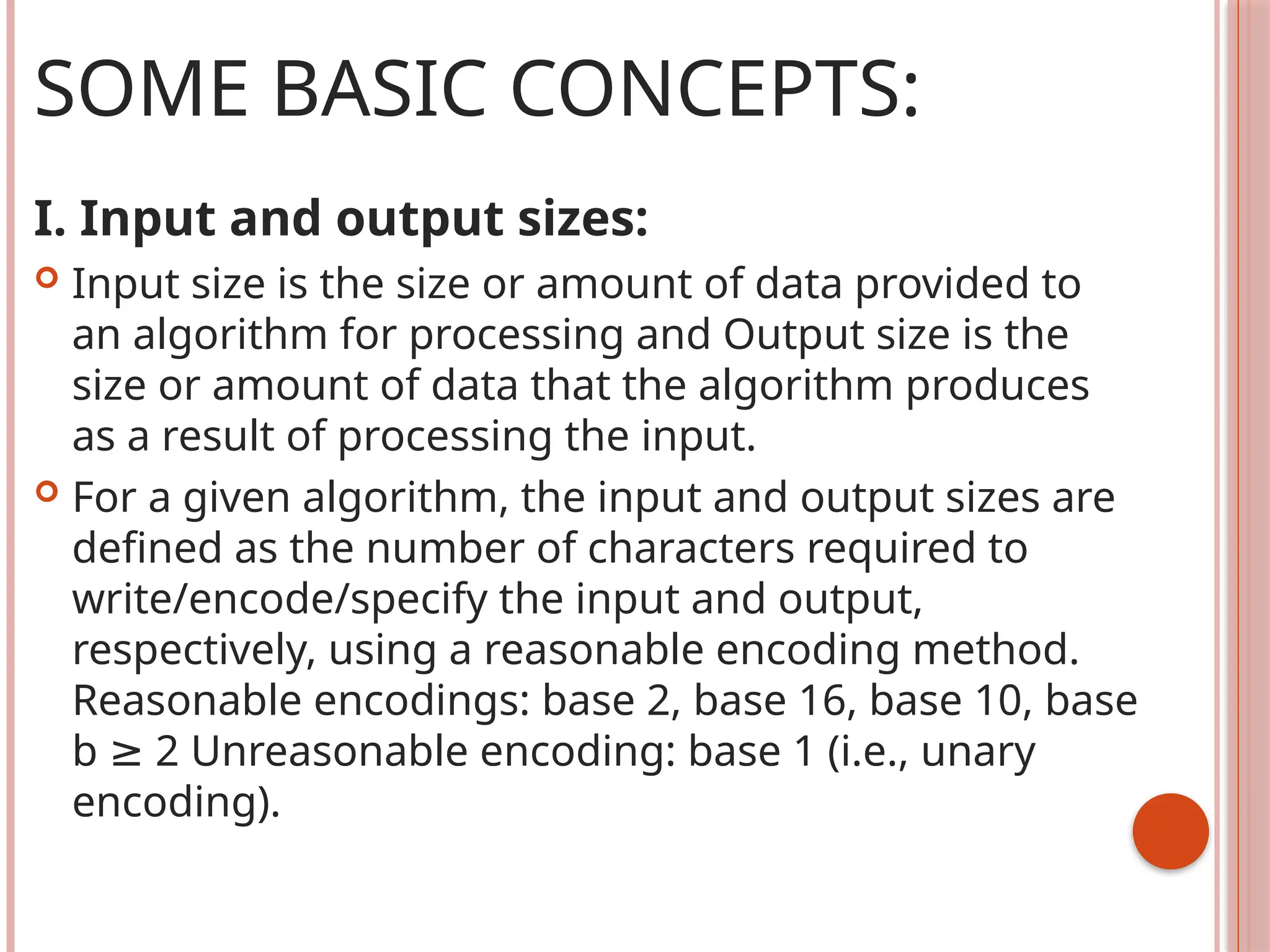
 Input size is the size or amount of data provided to
an algorithm for processing and Output size is the
size or amount of data that the algorithm produces
as a result of processing the input.
 For a given algorithm, the input and output sizes are
defined as the number of characters required to
write/encode/specify the input and output,
respectively, using a reasonable encoding method.
Reasonable encodings: base 2, base 16, base 10, base
b 2 Unreasonable encoding: base 1 (i.e., unary
≥
encoding).

2. II. Polynomial time algorithm:
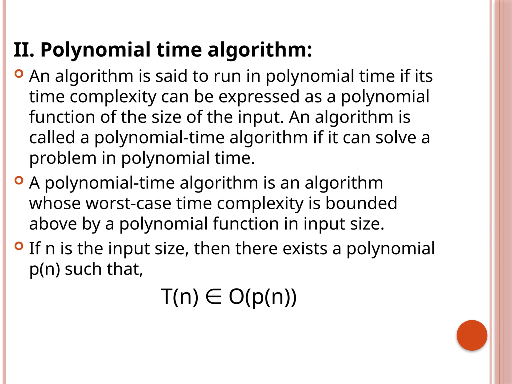
 An algorithm is said to run in polynomial time if its
time complexity can be expressed as a polynomial
function of the size of the input. An algorithm is
called a polynomial-time algorithm if it can solve a
problem in polynomial time.
 A polynomial-time algorithm is an algorithm
whose worst-case time complexity is bounded
above by a polynomial function in input size.
 If n is the input size, then there exists a polynomial
p(n) such that,
T(n) O(p(n))
∈

3. III. Hardness of problems:
1. Tractable Problems:
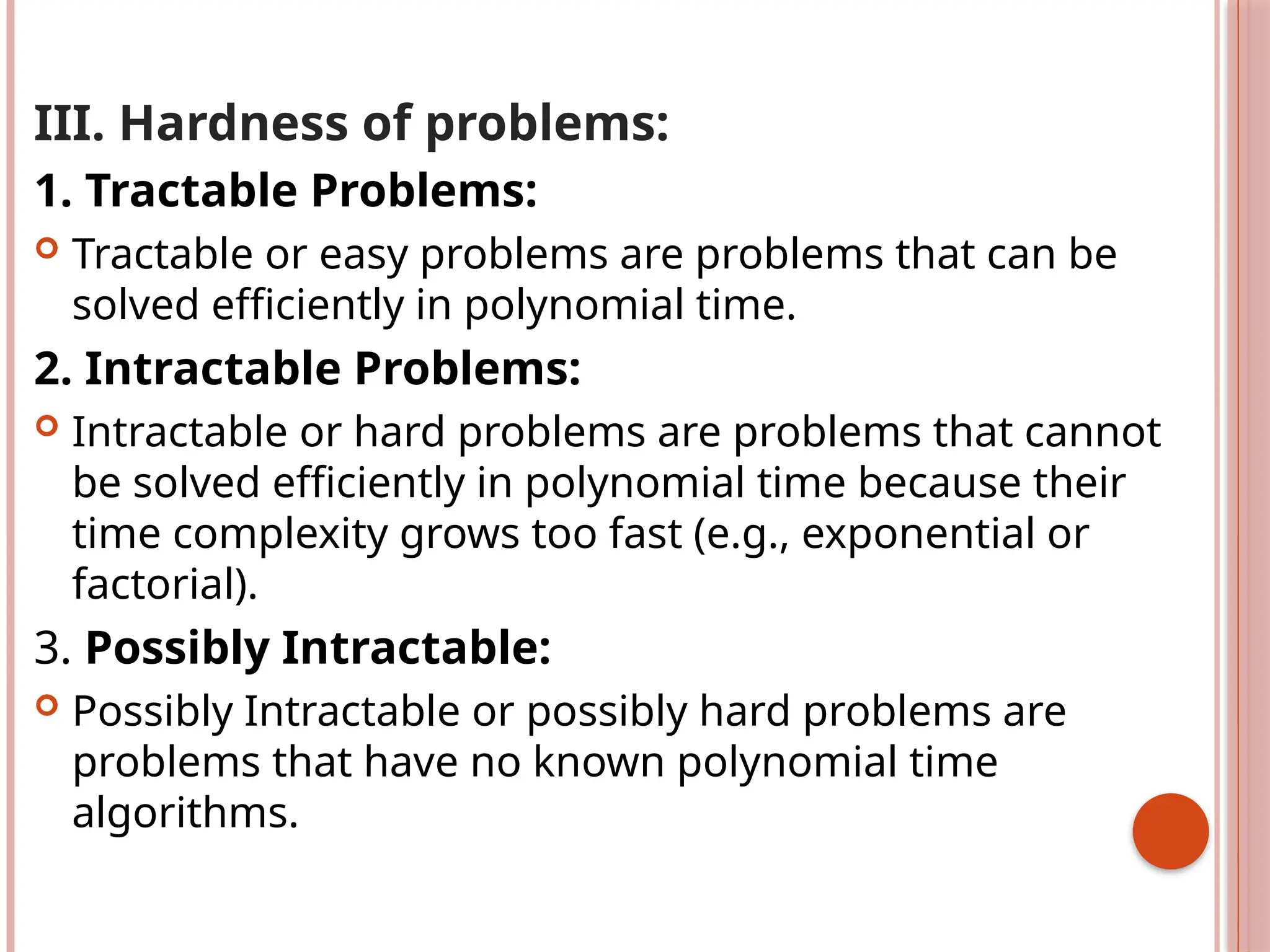
 Tractable or easy problems are problems that can be
solved efficiently in polynomial time.
2. Intractable Problems:
 Intractable or hard problems are problems that cannot
be solved efficiently in polynomial time because their
time complexity grows too fast (e.g., exponential or
factorial).
3. Possibly Intractable:
 Possibly Intractable or possibly hard problems are
problems that have no known polynomial time
algorithms.

4. CLASSIFICATION OF ALGORITHMS
I. Deterministic Algorithms:
 A deterministic algorithm is one where the behavior
is entirely predictable. Given a specific input, the
algorithm will always produce the same output and
follow the same sequence of steps. This predictability
makes deterministic algorithms reliable and consistent.
II. Non-Deterministic Algorithms:
 A non-deterministic algorithm is one where the
behavior can vary even with the same input. These
algorithms can produce different outputs on different
executions due to inherent randomness or multiple
possible execution paths.
In computer science, algorithms can be broadly classified
into two categories: deterministic and non-deterministic.

5. NON-DETERMINISTIC
ALGORITHMS
 A non-deterministic algorithm is a theoretical type of
algorithm that can try all possible solutions at the same
time and "guess" the correct one.
 These algorithms contain operations whose outcomes
are not uniquely defined but are limited to specified sets
of possibilities. The machine executing such operations
is allowed to choose any one of these outcomes subject
to a termination condition to be defined later. To specify
such algorithms, we use functions:
 Choice(S) - arbitrarily chooses one of the elements of set
S.
 Failure() – signals an unsuccessful completion.
 Success() – signals a successful completion.

6.  A non deterministic algorithm terminates
unsuccessfully if and only if there exists no set of
choices leading to a success signal. A machine capable
of executing a nondeterministic algorithm is called a
nondeterministic machine.
 For example: A nondeterministic algorithm for the
problem of searching for an element x in a given set of
elements A[1,n],n > 1 is given as,
1. j:=Choice(1,n);
2. if A[j] = x then{write(j); Success();}
3. write (0); Failure();
 From the way a nondeterministic algorithm
computation is defined ,it follows that the number 0 can
be output if and only if there is no j such that A[j] = x.

7. COMPLEXITY CLASSES
 In computer science, problems are divided into classes
known as Complexity Classes. In complexity theory, a
Complexity Class is a set of problems with related complexity.
With the help of complexity theory, we try to cover the
following.
 Problems that cannot be solved by computers.
 Problems that can be efficiently solved by computers.
 Problems for which no efficient solution exist.
 The common resources required by a solution are time and
space, meaning how much time the algorithm takes to solve
a problem and the corresponding memory usage.
 The time complexity of an algorithm is used to describe the
number of steps required to solve a problem, but it can also
be used to describe how long it takes to verify the answer.
 The space complexity of an algorithm describes how much
memory is required for the algorithm to operate.

8. TYPES OF COMPLEXITY CLASSES
I. P Class:
 The P in the P class stands for Polynomial Time. It
is the collection of decision problems that can be
solved by a deterministic machine in polynomial
time or problems solvable efficiently in polynomial
time by a deterministic algorithm.
 P is often a class of computational problems that
are solvable and tractable. Tractable means that
the problems that can be solved efficiently in
polynomial time .
 Example: Sorting a list using algorithms like
Merge Sort.

9. II. NP Class:
 The NP in NP class stands for Non-deterministic
Polynomial Time. It is the collection of decision
problems that can be solved by a non-deterministic
machine in polynomial time or problems where a
solution can be verified in polynomial time, but finding
the solution may not be efficient.
 The solutions of the NP class might be hard to find
since they are being solved by a non-deterministic
machine but the solutions are easy to verify.
 Problems of NP can be verified by a deterministic
machine in polynomial time.
 Example: The Satisfiability (SAT) problem.

10. III. NP-hard class:
 An NP-hard problem is at least as hard as the hardest
problem in NP and it is a class of problems such that
every problem in NP reduces to NP-hard.
 All NP-hard problems are not in NP.
 It takes a long time to check them. This means if a
solution for an NP-hard problem is given then it takes
a long time to check whether it is right or not.
 A problem A is in NP-hard if, for every problem L in
NP, there exists a polynomial-time reduction from L to
A.
 Example: Longest path problem in a graph.

11. IV. NP-complete class:
 A problem is NP-complete if it is both NP and NP-hard.
NP-complete problems are the hard problems in NP. If
any NP-complete problem is solvable in polynomial
time, then all NP problems are solvable in polynomial
time.
 NP-complete problems are special as any problem in NP
class can be transformed or reduced into NP-complete
problems in polynomial time.
 If one could solve an NP-complete problem in
polynomial time, then one could also solve any NP
problem in polynomial time.
 Example: Traveling Salesman Problem (decision
version).

12. NP-HARD PROBLEMS
I. Capacitated Network Design Problem (CNDP):
 CNDP involves designing a network with capacities assigned to
edges to meet certain demands between nodes, while
minimizing the overall cost.
 A coloring of a graph G = (V, E) is a function f : V → {1,2,...,k}
defined for all i belongs to V. If (u,v) belongs to E, then f(u) ≠
f{v).The chromatic number decision problem is to determine
whether G has a coloring for a given k.
 The problem is computationally challenging because:
 It requires finding an optimal combination of edges and
capacities to satisfy demands.
 The number of possible combinations grows exponentially
with the size of the graph..
 Solving CNDP exactly in polynomial time is not feasible unless P
= NP.
 The CNDP problem has applications in : Telecommunications,
Water Distribution Systems etc.

13. II. Directed Hamiltonian Cycle (DHC):
 A directed Hamiltonian cycle in a directed graph G = (V, E),
is a directed cycle of length n = |V|. A Hamiltonian cycle is
a cycle that visits each vertex in the graph exactly once
and returns to the starting vertex. The DHC problem is to
determine whether G has a directed Hamiltonian cycle.
 The problem is computationally challenging because:
 It requires checking all possible permutations of
vertices to determine if a Hamiltonian cycle exists.
 The number of permutations grows factorially with the
number of vertices, making it infeasible to solve
efficiently for large graphs.
 Solving DHC exactly in polynomial time is not possible
unless P = NP.
 The DHC problem has applications in : Traveling
Salesman Problem (TSP), Network Design, Scheduling etc.

14. III. Traveling Salesman Problem (TSP):
 TSP involves finding the shortest possible route that allows a
salesman (or any traveler) to visit a given set of cities exactly
once and return to the starting city.
 The decision problem is to determine whether a complete
directed graph G= (V,E) with edge costs c(u,v) has a tour of
cost at most M.
 Input: A weighted graph where nodes represent cities and
edge weights represent distances or costs.
 Output: A Hamiltonian cycle with the minimum total weight
(distance or cost).
 The problem is computationally challenging because:
 The problem requires evaluating all possible permutations
of cities (which grows factorially as n! for n cities)..
 There’s no known polynomial-time algorithm for solving it
unless P = NP.
 The TSP problem has applications in : Logistics and delivery
routing, Manufacturing ,DNA sequencing.

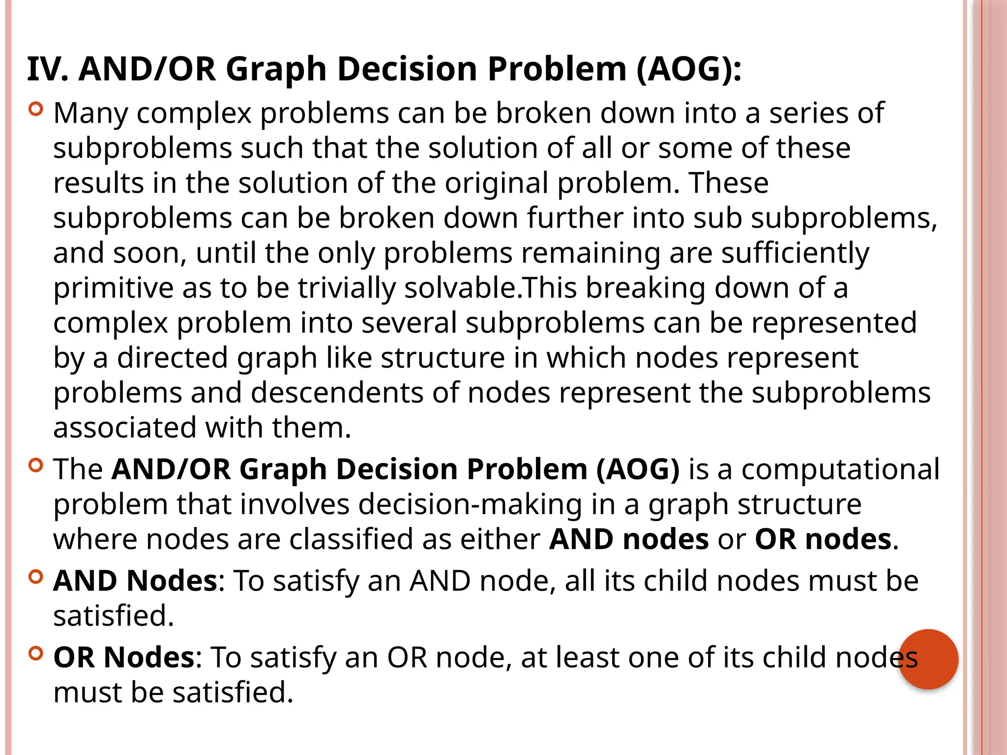
15. IV. AND/OR Graph Decision Problem (AOG):
 Many complex problems can be broken down into a series of
subproblems such that the solution of all or some of these
results in the solution of the original problem. These
subproblems can be broken down further into sub subproblems,
and soon, until the only problems remaining are sufficiently
primitive as to be trivially solvable.This breaking down of a
complex problem into several subproblems can be represented
by a directed graph like structure in which nodes represent
problems and descendents of nodes represent the subproblems
associated with them.
 The AND/OR Graph Decision Problem (AOG) is a computational
problem that involves decision-making in a graph structure
where nodes are classified as either AND nodes or OR nodes.
 AND Nodes: To satisfy an AND node, all its child nodes must be
satisfied.
 OR Nodes: To satisfy an OR node, at least one of its child nodes
must be satisfied.

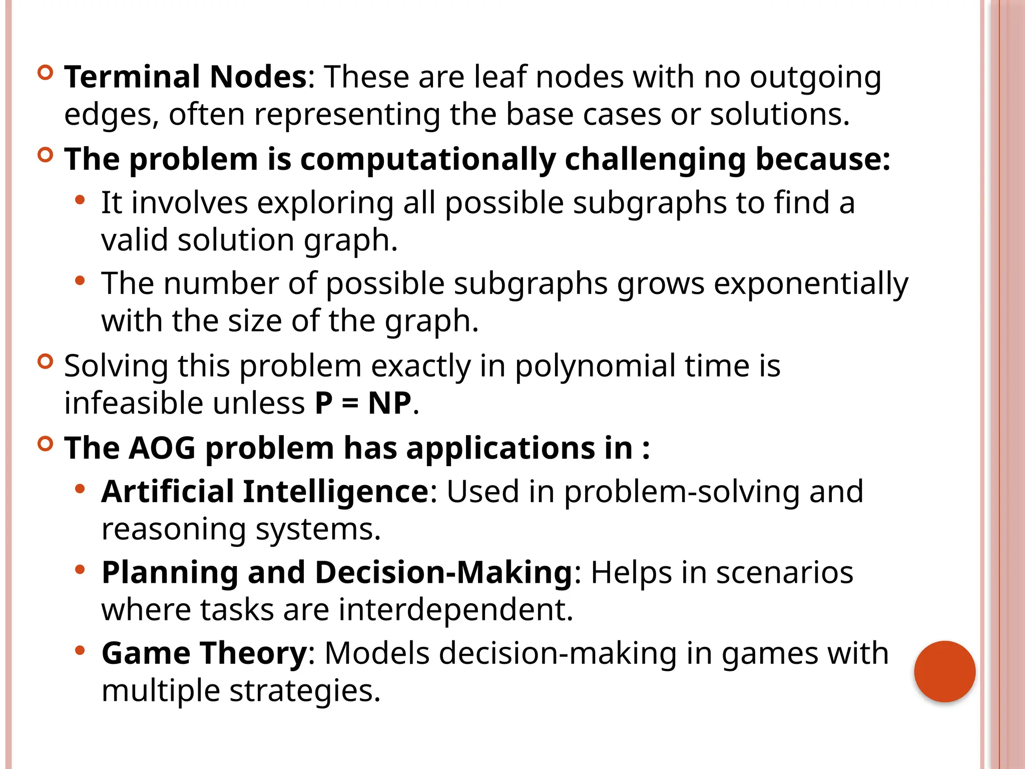
16.  Terminal Nodes: These are leaf nodes with no outgoing
edges, often representing the base cases or solutions.
 The problem is computationally challenging because:
 It involves exploring all possible subgraphs to find a
valid solution graph.
 The number of possible subgraphs grows exponentially
with the size of the graph.
 Solving this problem exactly in polynomial time is
infeasible unless P = NP.
 The AOG problem has applications in :
 Artificial Intelligence: Used in problem-solving and
reasoning systems.
 Planning and Decision-Making: Helps in scenarios
where tasks are interdependent.
 Game Theory: Models decision-making in games with
multiple strategies.