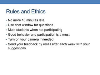
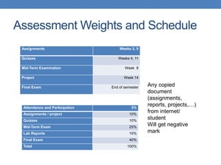
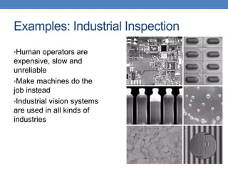
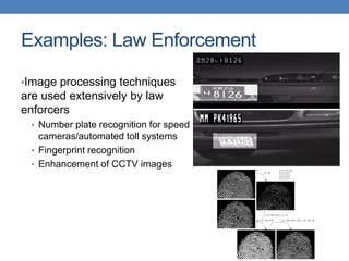
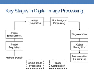
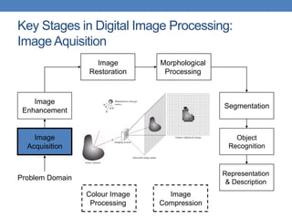
This document provides an introduction and overview of the CSE367 Digital Image Processing course. It outlines the rules and ethics for the course, the assessment weights and schedule, and potential article reading and project topics. It also lists some key journals and conferences in image processing. The lecture will cover an introduction to digital image processing, examples of applications, key processing stages, fundamentals of electromagnetic spectrum and light, image acquisition, representation, sampling and interpolation. Textbooks and extra materials are also referenced.

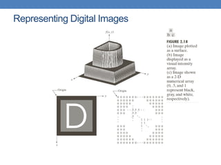
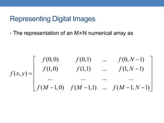
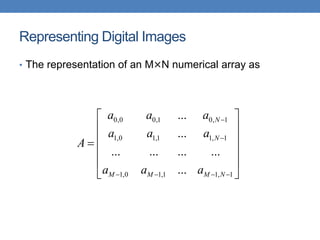
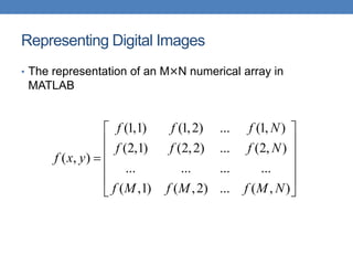
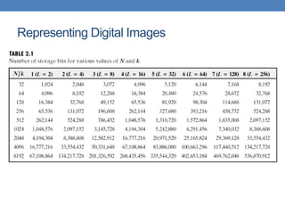
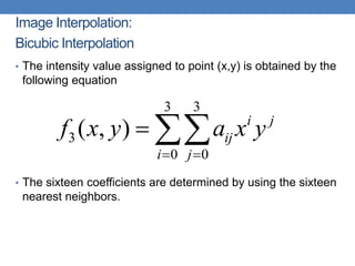
![Representing Digital Images
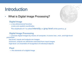
• Discrete intensity interval [0, L-1], L=2k
• The number b of bits required to store a M × N
digitized image
b = M × N × k](https://image.slidesharecdn.com/cse367lecture1-240220083834-b68fe356/85/CSE367-Lecture-1-image-processing-lecture-56-320.jpg)