Corruption-Draft 2

Abstract:
Corruption is commonly and universally thought to diminish societal welfare by constructing
a market operating via informal institutions perceived to be more efficient than the formal
institutions. Hayek, in The Road to Serfdom claims that “economic control is not merely control
of a sector of human life which can be separated from the rest; it is the control of the means for
all our ends.” Hayek’s belief that a controlled economy will result in our down fall is true to a
certain extent; not all corruption is ruthless. When an economy is centrally controlled there is
more of a chance of corruption to be present, with this corruption certain types assist in
lubricating the avenues by which the economy operates. This paper aims to determine whether
there is an optimal amount of corruption in a country that results in the highest wealth per capita
of its citizens. What is determined is that there is indeed a negative quadratic relationship
between corruption and welfare per capita; however, the results from the original equation have
lower t-statistics as interaction terms and other variables are included in the models. Also
determined was that increased corruption Granger causes welfare per capita, through a series of
regressions ranging from forty-four countries to one hundred fifty countries and data from 2008
to 2011.
Corruption in this paper is focused on bureaucratic corruption, which happens to be the most
popular type of corruption in many countries, particularly the less developed nations. Corruption
is defined as an “extra-legal institution used by individuals or groups to gain influence over the
actions of the bureaucracy” (Leff). Taking this further, it is assumed that the group or individuals
who hold influence are the ones that participate in the decision-making process to a larger degree
than normal, meaning that the people that have power are the ones that control the decision-
making process. This affects a country in numerous ways, namely in what the citizens of a
country receive from the government by way of infrastructure, education, and programs that are

2
geared toward creating wealth. Logically thinking, a more bureaucratically corrupt country will
have more control over what decisions are made, good or bad, and any proceeds from the bill
will hypothetically go into their pockets. Now a country with little or no corruption should
observe the same affect, however the means would be different in that the government does not
construct barriers to cash flows but the cash flows might be used in in less than desirable ways.
1. Introduction:
The effect of increased corruption on a country’s economy is ambiguous. Many argue that
corruption creates an extra-legal set of institutions that grinds the economy to a halt; while other
academics argue that in certain situations corruption can actually facilitate the growth of the
economy. The definition of corruption in this paper refers to the government and any
decentralized units (police, military, transit authorities, etc.) that abuse their entrusted power for
private gain, rather than use their power and funds to improve citizens’ lives.
Numerous academic papers have argued that corruption has a detrimental effect on the
economy and the growth of that economy. North (1990) claims that cumbersome and fraudulent
bureaucracies could possibly prohibit the distribution of permits and licenses, thus decreasing the
speed at which new processes become integrated into society. Mauro (1995) focuses on the
effects corruption has on business investment, finding that corruption decreases private
investment partly due to the risk involved of regime turnover, and the diminished property rights
that come with corruption. This lack of investment hampers the functioning of the economy and
its future growth if the corruption persists. Breaking this down further, Mauro explains that the
funds used to pay bribes to corruption officials could have been used in a more efficient manner.
Qerimi and Sergi (2012) analyze the Baltic nations and the relationship between corruption and
economic freedom. They find that the countries with the highest economic freedom scores also

3
made the most prominent progress in reducing corruption. Lastly, Susan Rose-Ackerman (1978)
and (2008) has investigated corruption and overall has theorized that corruption has a negative
effect on a country in that its citizens come to disregard some if not the majority of formal
institutions when there are informal laws that are much more efficient. This being said, nowhere
in her work does she claim that the informal institutions are necessarily better for the citizens,
there could be a possibility of higher crime, violence, and illicit markets that result from the lack
of control the government has over people’s lives.
On the other side, reasonable arguments have been made indicating that corruption can have
a positive effect and can facilitate the functioning of the economy when bureaucracies and
government fail to provide necessary institutions and goods to the public. Leff (1964) pioneered
this claim by arguing that corruption can have positive effects by ways of “speed money”, or
payments to bureaucrats for favors when institutions do not permit certain activities. Leff claims
that corruption is necessitated in situations when bureaucracies and government are indifferent
and/or hostile to their constituents or when government priorities do not match the public’s
priorities. When these situations are present, corruption acts as an operation to decrease
uncertainty, increasing investment as a result. Corruption is explained to aid innovation by
turning to government officials and making payments to secure property rights, increase
efficiency, and act as a hedge against bad policy with funds bypassing formal mechanisms and
bureaucratic red tape to get the money working faster.
Huntington (1968) follows Leff’s theory of how corruption can benefits society, claiming
that “order” is necessary for developing nations; this order however does not have to be created
or maintained through formal institutions. There are possibilities where the legislation is not
orderly and the informal institutions present that order necessary to help the economy function.

4
For example, after World War II in mainland Europe, the total destruction disabled the ports and
farmland was rendered useless, citizens were subject to rationing and with an interim
government of the allied forces that was more a police force, citizens were forced to buy good
outside of what the ration books provided on the black market, to bribe ration officials for extra
rations, or by looting, this market provided more goods, more efficiently to the citizens than the
rationing books (Gollehon, 2014). Another advocate of beneficial corruption, Carden and Verdon
(2010) analyze the view that all corruption is bad by examining corruption by country for
different segments (military, education, business, the legal system, police, and tax). Of those
different segments, only business corruption is shown to increase economic growth conditional
on the country being economically less free than every other segment, and had a negative
association between corruption and economic growth. In other words, the business industry
benefits from corruption in that if there is are prohibitive levels of bureaucratic red tape or less
economically free areas, corruption in business would lead to more activity in the economy than
if abiding by the red tape.
The main goal of this paper is to, rather than looking for a linear pattern of the relationship
between corruption and wealth per capita, look to find a level of corruption that results in the
highest welfare per capita. The effect is somewhat similar to the Laffer curve, where there is an
unknown amount of the tax rate that results in the largest amount of revenues; in this case there
is some value of the Corruption Perception Index that results in the largest welfare per capita.
This paper proceeds as follows, section 2 sets out the definitions of corruption, economic
freedom, and the hypothetical implications of the study; section 3 provides an in depth analysis
of the data used and it’s limitations; section 4 talks about the empirical estimations of the paper;
and section 5 analyzes the results from the regression.

5
2. Conditions
Before proceeding into an in depth analysis of the results, there are some conditions that need
to be mentioned, first is the definition of corruption and how it relates to the paper, the definition
of economic freedom and how it relates to the paper, the definitions of institutions, and the
hypothetical implications of each.
The underlying theory is that if one country had a corruption score of zero represents a
country that is completely corrupt, where bureaucrats are present in many facets of daily life, the
government or formal institutions are not strong in the presence of its citizens and there are
minimal institutions that protect people and their property rights. Hypothetically, a country at the
max wealth per capita would have a corruption score that falls between the two scores, and
represents an economy where there is just enough corruption where red tape is maneuvered
around and helps speed the economy through not completely legal methods, but there is still a
basic trust in the governing body and institutions that protect property rights and fosters
innovation and investment.
The following examples of how too much and too little corruption can have negative effects
on the economy. An example is when there a patent on a product that could increase the
harvesting capacity to the degree that the current practice is obsolete. A country with minimal
corruption and largely agricultural, might not see the patent come through the systems because
the money that would be used to develop it could possibly have been used elsewhere. The same
country, now with a large amount of corruption, might not see the patent submitted for approval
because of the “fee” required by the inventor is not available to him. Either way results in the
economy suffering from not seeing a more efficient method being approved because the patent
was not submitted due to the institutions.

6
Economic freedom in this paper is also argued to be an alternative measure of the degree of
bureaucratic corruption. This freedom is defined as “the absence of government constraint or
coercion on the production, distribution, or consumption of goods and services beyond the extent
that is necessary for citizens to protect and maintain liberty itself” (O’Driscoll, Fuelner, and
O’Grady, 2003). Applying this to corruption and welfare per capita, the less corruption that is
present in that country, the more options available for citizens to spend money. What I expect to
find is a positive relationship between corruption and economic freedom. This relationship is
then extended to support the claim of a positive relationship between economic freedom and
overall economic growth, which Ayal and Karras (1998), Gwartney, Lawson, and Holcombe
(1999), De Haan and Sturm (2000), and Carlsson and Lundström (2002) have each determined.
One final note concerning the use of terminology is needed. Rather than referring to laws or
bills passed by the legislative body or decrees from the supreme ruler, the term institutions refers
lifestyles, ethics, and rules of which society operates; an example would be how well governing
agencies protect its citizens and their property rights, and foster a fair market place. There are
two types of institutions that addressed in this paper, formal and informal. Formal institutions
which are institutions that are set up in the constitution formally stated and enforced by
government. Informal institutions are ways of life that are not from the government, but take
place on a very normal basis. Some examples would be the corruption of government officials in
order to speed things through red tape; cars going overtly fast on a road where it is common
knowledge that no cops are present, both of these examples involve people disobeying written
rules and following rules that are common knowledge or are generally accepted by the public.
3. Data Description

7
The data for this paper is drawn from four different sources, the Corruption Perception Index,
Gross Domestic Product per Capita net government spending and the Gini coefficients for each
country available from the World Bank, and the Economic Freedom score for each country from
the Heritage Foundation.
The primary measure used to quantify corruption is the annual Corruption Perception Index
created by Transparency.org. This index ranks the countries used in this paper based on how
corrupt the citizens in that country perceive the public sector to be. A scale of one to one hundred
is used and the higher the score the less corrupt a country’s government is perceived to be. In the
indices prior to 2012 the scale ranged from zero to ten and to bring those scores to the same scale
as the current measures, a factor of ten was multiplied to the older scores. The rating is
determined relative to other countries and territories included in this index. This index was used
in order to quantify the level of corruption in a country and to determine whether there is a
relationship between corruption and wealth per capita in regression analysis and to show if there
is an optimal level of corruption. The theory behind using this measure and the square was that a
more corrupt country and a less corrupt country will have less wealth per capita, relative to a
country that has some corruption that helps speed up production or investment. For this paper,
every index back to the original index in 1995 was used to use for more inclusive data and for
the effects of changes in corruption on the welfare per capita.
The gross domestic product per capita from the World Bank was used as a primary measure
of wealth per capita. One modification to this measure was to subtract out government spending
per capita since this paper focuses on the impact from changes in institutional quality on private
sector performance, included government spending would lead to an endogeneity bias. This
value was calculated by dividing the government spending per year (in current US dollars) by the

8
population and then subtracted the quotient from the GDP per capita. This number is recorded in
current US dollars and quantifies how wealthy a country’s citizens are. The reasoning behind
using this measure is that it accounts for the size of a country’s economy by spreading it out
among its citizens. Obviously a large country, like the United States, will have a larger gross
domestic product than of Benin or Armenia; however, the per capita measure may not have the
same conclusion. In other words the per capita scaling allows for size of economy to be
dismissed and allows for a more direct relationship between corruption and its effect on its
citizens. The hypothetical relationship between gross domestic product per capita and the
Corruption Perception Index would be that the highest per capita gross domestic product should
fall somewhere around the average of the index scores.
The Gini index, from the World Bank databank, measures the extent that a country’s income
distribution or consumption from individual households in an economy deviates from an equal
distribution. As part of this index, the Lorenz curve for each country plots the cumulative percent
of income earned on the cumulative percent of people from lowest income to highest income.
Since a perfect distribution is very rare, the area between the perfect distribution and the Lorenz
curve creates the Gini index, or the percent of deviation from the perfect distribution line. The
Gini index measure is used along with the corruption perception index scores can show a
relationship between income distribution and corruption; meaning in countries with a very
unequal income distribution, the majority of wealth is held by a smaller percent of the citizens;
this small group having extreme wealth could stem from graft or wealth being held by
bureaucrats. Having the Gini index included along with corruption scores and their squares
would allow for an aspect of corruption based on income distribution. The data used in this paper
begins in 1995 because this is the year when the Corruption Perception Index was first created;

9
however, the Gini coefficient for many countries was not taken on an annual scale and became
the variable that limited the amount of entries for the final data set.
The final measure was the Economic Freedom of each country provided by the Heritage
Foundation. This index measures ten components of economic freedom: business freedom, trade
freedom, fiscal freedom, government spending, monetary freedom, investment freedom,
financial freedom, property rights, freedom from corruption, and labor freedom (O’Driscoll,
Feulner, O’Grady, 2003). This measure was used as a supplement to corruption because
increased economic freedom in an economy is associated with an increase per capita wealth
along with “a variety of positive social and economic goals” (O’Driscoll, Feulner, O’Grady,
2003). This paired with the corruption measure will add another dimension to relationship of
wealth per capita in the regression that would account for the ability of the citizens to not only
control their property, but also for movement of investments. Hypothetically, a less economically
free country has power that is centralized and has a larger government intervention in the
economy, and that is correlated with increased probability of corruption since the people have
less control of what they can do with their money.
There are some obstacles when it comes to the data that is being used in this paper, there is the
obvious issue of subjectivity in certain measures, scaling changes from prior editions of the
indices, and measures that have not been updated in quite some time. The subjectivity issues
becomes a concern in the data on corruption and the economic freedom scores. The corruption
perception index is created based on the perception of a country’s government; the economic
freedom scores are also subjective in the sense that scores are derived partly by qualitative
measures and not strictly quantitative measures. This subjectivity can result in biasedness of
scores results in inaccurate data. Another issue with the data is that some countries did not have

10
scores for Gini coefficients that were successive on periodic, or these countries were missing
values completely. Not having periodic scores creates a discrepancy in the data, in that Gini
scores may have changed drastically since the last recording and regression analysis may not
accurately describe the relationship between corruption and welfare since those values had to be
eliminated. The missing values resulted in a shrinking of the data set from over one thousand
data points to around seven hundred values; this was not an issue solely with the Gini, the CPI
did not have measures on all countries since 1995, rather it started around fifty and then grew
steadily to become all inclusive. A final issue with the data was scaling changes on the
corruption measure, some of the data did not have the most current corruption scores an attempt
was made to get corruption scores for years where the Gini index was last recorded; a scaling
change between 2011 and 2012 made scores lie on a scale of zero to one hundred rather than the
original scale of zero to ten. This was overcome, as mentioned earlier, by scaling older values by
ten. Descriptive statistics of all included variables can be found in Table 1.
Table 1: Descriptive Statistics of Data Set
Mean
Standard
Deviation Minimum Maximum
Corruption Perception Index 40.034 18.977 15 100
Corruption Perception Index^2 1962.818 2021.762 225 10000
GINI 40.421 10.027 16.23 67.4
Gross Domestic Product per Capita $6,914.79 $9,757.18 $3.69 $67,460.36
Economic Freedom 61.006 9.497 24.3 89.9
4. Empirical Estimates
This section analyzes the plots between certain variables to determine the relationship relative
to presiding theories (4.1), the general regression of the theory and modification to the equation
(4.2 to 4.6), the regression between corruption and Gini (4.7), and the Granger-Causality
regressions (4.8).

11
4.1 Plots
The xy-plots below provides an overview of the relationships of Gini and corruption (4.1.1),
economic freedom and corruption (4.1.2), economic freedom and Gini values (4.1.3), and
welfare per capita values to corruption (4.1.4). There are 683 values that come from over 150
countries with data entries ranging from 1995 to 2013, not all of the countries had values from
1995 to 2013, the limiting factors were the Gini coefficients from the World Bank database since
many countries have those numbers every four or five years, and the Corruption Perception
Index from Transparency international since the study was founded in 1995 and was limited to
only fifty countries.
4.1.1: Gini to Corruption
The relationship between Gini and Corruption is hypothetically negative. This is relationship
is reasonable in the sense that the as the corruption perception value increases (a country is more
clean from corruption), there should be less inequality of distribution (or more equality) as the
Lorenz curve becomes closer to the equal distribution line.
When the Gini scores are plotted against corruption as a second order polynomial the
resulting curve shows that there is a value of corruption that maximizes Gini, and the fit of data
is slightly better. The data appear to have a funneling shape to it, the data are very spread out
when the closer to the origin, however when moving away from the origin, the data tends to be
less variable, one reason could be that few countries have corruption perception scores higher
than 80 and many tend to fall between 20 and 50. This wide range of values has the ability to
take on a large amount of Gini values and could account for the pattern seen and with that large
range of Gini values a lower R2 value relative to other plots shown below.

12
4.1.2: Economic Freedom and Corruption
The relationship, much like the Gini index analysis previously, is logical. At first glance, it
shows that as corruption perception increases so does the economic freedom scores. This is
relationship is supporting numerous studies mentioned previously that show economic freedom
and corruption are negatively associated. That being said, as the corruption perception value
increases, there should be more economic freedom. The same process was taken and plotting the
Economic Freedom Scores against the second order polynomial of Corruption. The resulting
curve shows that there is a value of corruption that maximizes Economic Freedom, and the fit of
data is again slightly better. The relative maximum of this function for corruption is
approximately 91.42, and an Economic Freedom value of 72.25. The same pattern is present as
with the Gini coefficient and corruption, where it becomes more concentrated in the spread of
values as corruption perception scores increase.
y = -0.1184x + 45.182
R² = 0.0501
0
20
40
60
80
0 20 40 60 80 100 120
GiniIndex
Corruption Percpetion Score
Gini to Corruption
y = -0.0038x2
+ 0.2762x + 36.811
R² = 0.0732
0
20
40
60
80
0 20 40 60 80 100 120
GiniIndex
Corruption Percpetion
Gini to Corruption

13
4.1.3: Economic Freedom and Gini
The relationship between EF and Gini is almost nonexistent, and if there is one it would be
essentially a flat line. The R2 value for the relationship is 0.0045, the slope is slightly negative
but less than 0.10. Since the trend line has a slope of approximately zero, I view these terms as
interchangeable. What the lack of a correlation could mean is that Gini values and economic
freedom values cannot be predicted from the other or that economic freedom at a certain level
implies a Gini at another. According to the trend line, it appears that lower Gini values, or more
equality of income, are associated with higher economic freedom values. Which is pragmatic
sense if more a country has a more equality in its income distribution, there is not a minority of
y = 0.3023x + 48.823
R² = 0.345
0.0
20.0
40.0
60.0
80.0
100.0
0 20 40 60 80 100 120
EconomicFreedom
Corruption
EF to Corruption
y = -0.0038x2
+ 0.6948x + 40.499
R² = 0.369
0.0
20.0
40.0
60.0
80.0
100.0
0 20 40 60 80 100 120
EconomicFreedom
Corruption
EF on Corruption

14
people that control the majority of the money, and thus there is more economic freedom for the
citizens and less opportunities for corruption to develop.
4.1.4: Welfare per Capita and Corruption
With the welfare per capita and corruption relationship, it seems obvious that as corruption
decrease net welfare per capita increases. That’s the very point that the first xy scatter plot
illustrates. The less corruption in a society, the more money that people are able to spend rather
than having to spend it to get through red tape. The first trend line is a linear relationship, and
has a very high R2 value, however for the data set used the lower bound was not negative, thus
plotting it on the quadratic of corruption the R2 increases approximately 5%. At the tail end of
the graph however, the data has a pattern of dispersing. This could mean that there are more data
points where corruption is higher and welfare per capita is lower relative to low corruption and
high net welfare per capita countries, or the claim that lower corruption leads to higher welfare
per capita is entirely correct. Looking at the overall trend that appears to be the case, however,
looking at Corruption scores of 60 and above, the variance of the data points greatly increases
there appear to be just as many points below the trend line as there are above meaning many of
the countries suffer from lower than expected welfare per capita values with lower corruption.
y = -0.0653x + 63.559
R² = 0.0045
0.0
20.0
40.0
60.0
80.0
100.0
0 10 20 30 40 50 60 70 80
EconomicFreedom
Gini Coefficient
EF to GINI

15
4.2 General Regression
The theory behind this paper, as mentioned previously, is to find a negative quadratic
relationship between welfare per capita and corruption. The first equation output, below,
contains, simply, the welfare per capita ran against corruption perception and its square. What it
shows is that there is an extremely significant relationship between corruption, corruption
squared, and welfare per capita. One of the reasons why these variables are so highly significant
is that the unobserved errors are contained in the constant, thus by adding other variables that
could help predict corruption or at least the possibility of corruption would help make this
regression more robust.
Based on this equation, the “optimal” amount of corruption appears to be 83.31, which is
representative of very low level of corruption in a country. This corruption value corresponds to
a welfare per capita value of $1815.26, which is very low considering the average welfare per
y = 394.56x - 8876.2
R² = 0.5898
-$10,000.00
$0.00
$10,000.00
$20,000.00
$30,000.00
$40,000.00
$50,000.00
$60,000.00
$70,000.00
$80,000.00
0 20 40 60 80 100 120
Welfare per Capita to Corruption
y = 5.1203x2 - 139.68x + 2455.7
R² = 0.6346
$0.00
$20,000.00
$40,000.00
$60,000.00
$80,000.00
0 20 40 60 80 100 120
Welfare per Capita to Corruption

16
capita value was closer to $7,000. This is accounted for by having a data set for welfare per
capita that has a very large variance, in this case it was close to $95,000, (Table 2) and in this
situation this data was skewed to the right with the majority of the values falling below $10,000.
How this relates to the data used to compute this regression, the maximum corruption value falls
above the seventy-fifth percentile, and while the welfare per capita values falls between the
twenty-fifth and fiftieth percentile. One other noticeable factor is the R2 value, it is a respectable
35% (Table 2, Model 1) and shows that there is some resemblance of a trend between corruption,
its square, and welfare per capita.
4.3 Original Regression with Gini and Economic Freedom
After analyzing the first equation, the next step was to add some variables that could imply
some sort of corruption based on their values; thus, the Gini Coefficients and the economic
freedom scores were added; since a larger Gini hints at more corruption and more economic
freedom hints at lower corruption and to help account for variations in the data. The output in
Table 2, Model 2, contains the regression that has the Gini and economic freedom values. The
results show that Gini is extremely significant when predicting welfare per capita, however, the
CPI and its square are no longer significant at the 1% percent level, but they are significant only
at the 10% level. This shows that once accounting for other measures of corruption the
corruption index values lose weight when it comes to predicting welfare per capita. The
following changes to the regression will be squaring Economic Freedom, adding an interaction
term between corruption and economic freedom, and adding both the square of Economic
Freedom and the interaction term.
After analyzing the first equation, the next step was to add some variables that could imply
some sort of corruption based on their values; thus, the Gini Coefficients and the economic

17
freedom scores were added; since a larger Gini hints at more corruption and more economic
freedom hints at lower corruption and to help account for variations in the data. The output
below, contains the regression that has the Gini and economic freedom values. The results show
that Gini is extremely significant when predicting welfare per capita, however, the CPI and its
square are no longer significant at the 1% percent level, but they are significant only at the 10%
level (Table 2). This shows that once accounting for other measures of corruption the corruption
index values lose weight when it comes to predicting welfare per capita. The following changes
to the regression will be squaring Economic Freedom, adding an interaction term between
corruption and economic freedom, and adding both the square of Economic Freedom and the
interaction term.
4.4 Economic Freedom Squared
The following regression ran contained the variable of economic freedom squared replacing
corruption squared. This was to see, if an alternative measure of corruption would render the
same results with the same significance as the original equation.
What is determined that both economic freedom and economic freedom squared are
extremely significant at the 1% level, the same reasoning applies with the original equation,
however, one thing that differs is that the R2 value for this equation is significantly higher at
88.43% (Table 2, Model 3), obviously this model is a much better fit for this data than using a
direct corruption scores.
What is determined that both economic freedom and economic freedom squared are
extremely significant at the 1% level, the same reasoning applies with the original equation,
however, one thing that differs is that the R2 value for this equation is significantly higher at

18
88.43% (Table 2), obviously this model is a much better fit for this data than using a direct
corruption scores.
After analyzing the first equation, the Gini and corruption perception index values were
added to the model to directly account for corruption and another measure that could help
account for the welfare per capita given the distribution of income. The results of the new
equation are astounding, economic freedom and its square are still extremely significant at the
1% level and have slightly more drastic t-statistics which show a stronger relationship ship
between economic freedom and welfare per capita and that economic freedom is a very accurate
predictor of welfare per capita (Table 2, Model 4). Comparing this regression to the one above,
the R2 values are almost identical, the slope coefficients for both economic freedom and its
square are nearly identical, and corruption is significant at the 10% level, and Gini is no longer
significant relative to when corruption was squared (Table 2 Model 4).
Table 2: Ordinary Least Squares Estimatesof GDP perCapita, Year
Model 1 Model 2 Model 3 Model 4
Coefficient Coefficient Coefficient Coefficient
Constant
-85.626
** 334.967
***
-
1496.750 *** -1500.280
***
(36.048) (65.215) (75.685) (73.574)
Corruption Percpetion Index 14.592 *** 3.473 * 0.336 *
(1.595) (2.068) (0.171)
Corruption Perception Index^2 -0.0840 *** -0.0328 *
(0.015) (0.0189)
Gini -2.467 *** -0.186
(0.768) (0.262)
Economic Freedom 0.437 40.744 *** 41.072 ***
(0.987) (2.358) (2.371)
Economic Freedom^2 -0.172 *** -0.178 ***
(0.019) (0.019)
R^2 0.351 0.020 0.885 0.885
Observations 683 683 683 683
Notes: Standard errors inparentheses. Statisticalsignificanceat1%,5%,and 10% denoted by ***, **, and *, respectively.

19
4.5 Original Regression with Interaction Term
The next step in the analysis was to add an interaction term between corruption and
economic freedom. The reasoning behind adding this interaction term was to see if the
relationship between corruption perception or economic freedom and welfare per capita is
different at different values of the other explanatory variable. Meaning that, it would help us to
determine if there is a larger or smaller effect of corruption perception on welfare per capita if
economic freedom decreases.
The coefficient for this interaction term should be positive, since the increasing corruption
perception score signifies lower corruption, and a higher economic freedom score is better. The
coefficient from the regression output however is negative and significant at the 1% level (Table
3, Model 5). Additionally, CPI2 becomes statistically significant at the 10% level (Table 3,
Model 5) but does not have a negative sign with it, which would signify that the equation is
flipped, and Gini variable is no longer significant at the 1% level (Table 3, Model 5).
4.6 Economic Freedom Squared and Interaction Term
The next regression performed involves economic freedom and its square with an interaction
term between economic freedom and corruption perception. With these calculations, it shows
that economic freedom is a more robust variable than corruption perception and can be viewed as
a substitute to corruption.
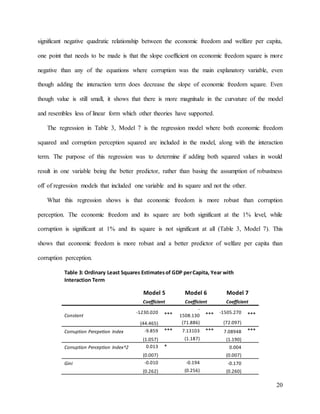
Since economic freedom can be viewed as a better predictor of welfare per capita, Table 3
Model 6 shows that every variable except the Gini coefficients were significant at the 1% level
and results in a higher adjusted R2 value than before. This regression shows that there is a

20
significant negative quadratic relationship between the economic freedom and welfare per capita,
one point that needs to be made is that the slope coefficient on economic freedom square is more
negative than any of the equations where corruption was the main explanatory variable, even
though adding the interaction term does decrease the slope of economic freedom square. Even
though value is still small, it shows that there is more magnitude in the curvature of the model
and resembles less of linear form which other theories have supported.
The regression in Table 3, Model 7 is the regression model where both economic freedom
squared and corruption perception squared are included in the model, along with the interaction
term. The purpose of this regression was to determine if adding both squared values in would
result in one variable being the better predictor, rather than basing the assumption of robustness
off of regression models that included one variable and its square and not the other.
What this regression shows is that economic freedom is more robust than corruption
perception. The economic freedom and its square are both significant at the 1% level, while
corruption is significant at 1% and its square is not significant at all (Table 3, Model 7). This
shows that economic freedom is more robust and a better predictor of welfare per capita than
corruption perception.
Table 3: Ordinary Least Squares Estimatesof GDP perCapita, Year with
Interaction Term
Model 5 Model 6 Model 7
Coefficient Coefficient Coefficient
Constant
-1230.020 ***
-
1508.130 *** -1505.270 ***
(44.465) (71.886) (72.097)
Corruption Percpetion Index -9.859 *** 7.13103 *** 7.08948 ***
(1.057) (1.187) (1.190)
Corruption Perception Index^2 0.013 * 0.004
(0.007) (0.007)
Gini -0.010 -0.194 -0.170
(0.262) (0.256) (0.260)

21
Economic Freedom 25.680 *** 36.869 *** 36.757 ***
(0.802) (2.428) (2.437)
Economic Freedom^2 -0.111 *** -0.108 ***
(0.022) (0.022)
Interaction Term of CPI and EF -0.166 *** -0.103 *** -0.109 ***
(0.017) (0.018) (0.021)
R^2 0.887 0.891 0.891
Observations 683 683 683
Notes: Standard errors inparentheses. Statisticalsignificanceat1%,5%,and 10% denoted by ***, **, and *,
respectively.
4.7 Corruption and Gini Regression
One additional regression that needed to be modeled was that of corruption and its square on
Gini coefficients. This was to see if there is a negative quadratic relationship between the three
variables.
The results in Table 4, shows that indeed there is a negative quadratic relationship between
corruption and Gini, and both the corruption and its square variable coefficients are significant at
the 1% level, this is the same output as the xy-scatter plot presented previously. What is seen is
that corruption and its square are both extremely significant at the 1% level. this equation was
derived to determine the relative max of corruption and the corresponding Gini value in this
function, which was determined to be approximately 36.34, and the Gini value of 41.83; the
trend is that when corruption is lower (closer to 30), the Gini tends to be higher (less equal in
distribution) which is logical.
The result, as shown below, shows that indeed there is a negative quadratic relationship
between corruption and Gini, and both the corruption and its square variable coefficients are
significant at the 1% level, this is the same output as the xy-scatter plot presented previously
(Table 4). What is seen is that corruption and its square are both extremely significant at the 1%

22
level (Table 4). this equation was derived to determine the relative max of corruption and the
corresponding Gini value in this function, which was determined to be approximately 36.34, and
the Gini value of 41.83; the trend is that when corruption is lower (closer to 30), the Gini tends to
be higher (less equal in distribution) which is logical.
Table 4: Ordinary Least Squares
Estimates ofGini Coefficient
Model 8
DV: GINI Coefficient
Constant 36.824 ***
(2.210)
Corruption Percpetion Index 0.276 ***
(0.098)
Corruption Perception
Index^2
-0.004
***
(0.001)
R^2 0.885
Observations 683
Notes: Standard errors inparentheses. Statistical
significanceat 1%, 5%, and 10%denotedby ***, **,
and *, respectively.
4.8 Granger-Causality Results
After determining that there is a negative quadratic relationship between corruption and
welfare per capita and that it was robust when modifying the original equation to add Gini,
economic freedom, the square of economic freedom, an interaction term, and the square of
economic freedom and the interaction term; the next move was to determine whether or not there
is a causal relationship between corruption and welfare per capita.
Starting out, an issue of how many lags used to run this test was solved by running a test with
three year lags (2008-2010 and using the current period as 2011), and two year lags with the

23
same current period. Also, of the 683 data points used in the first regression, only forty-three
countries, after reduction had values for both welfare per capita and corruption for 2008 to 2011.
To make sure that any significant F-stats were not due to limited data, all 150 countries from the
original data set were included in another test with welfare per capita values and corruption and
are referred to complete. Thus, there were four data sets to test for Granger-Causality, 3yr lags,
2yr lags, and; and there were four regressions run, each data set had two regressions, one with
corruption as the dependent variable and the other as welfare per capita as the dependent
variable.
After performing the regression analysis, what is found is that all of the F-statistics where the
corruption perception index was the dependent variable were not significant. With respect to the
regressions where the welfare per capita values were used every regression. Thus proving that
one side causality is evident with corruption granger-causing welfare per capita. These tables are
exhibits at the end of this paper. The next process in the Granger-Causality analysis is to see if
the growth rates of welfare per capita and corruption from year to year would provide more
evidence of causality between corruption and welfare per capita. The growth rates were annual
growth rates of two year lags using the growth from the three year lag data. The results did not
expose any new results, even results supporting the original causality statement. All the F-
statistics were insignificant at the 5% level. These tables are located in the exhibits at the end of
this paper after the original causality results.
Since it was determined earlier that economic freedom is a substitute for corruption
perception, the same Granger-Causality tests were performed on the data to see if there was one
side causality between economic freedom and welfare per capita. The results were inconclusive,
the only test that came back significant at the 5% level was the two year lags with welfare per

24
capita as the dependent variable. What this concludes is that there is no evidence supporting the
claim that economic freedom Granger-Causes welfare per capita.
Concluding Remarks and Basis for Future Research
This paper analyzed the effects of corruption on welfare per capita for numerous countries
over a span of eighteen years in an attempt to determine if there is a negative quadratic
relationship between corruption and welfare per capita and if there is a causal relationship
between them as well. This paper researches a view that is opposite of a more accepted view,
where there is a negative linear relationship between corruption and welfare per capita.
What is found is, at first glance, that there is an extremely significant relationship between
the corruption and welfare, however, as other measurements of corruption are accounted for in
the model (Gini and economic freedom), the significance of corruption and its square is reduced.
In further research, this paper shows that between corruption and the Gini coefficient there is
significant negative quadratic relationship; and when substituting economic freedom for
corruption perception the model becomes more robust with the coefficients remaining
statistically significant at the 1% level with Gini and corruption values added, adding an
interaction term of economic freedom and corruption, and when adding corruption and its square
to the equation. Another aspect of this paper was to determine if there was a causal relationship
between corruption and welfare per capita, what is found is that corruption Granger-Causes
welfare per capita for every regression except when the 2yr lags of forty-four countries were
statistically significant at the 5% level.
This paper could be further developed into determining whether countries with more
emphasis on a certain industry sector (agriculture, services, manufacturing) result in more
corruption and if that relationship has an effect on welfare per capita. This would help explain

25
countries with a higher emphasis on agriculture there may tend to be lower values of welfare per
capita because the countries may not be as developed or mature as other nations. A second
development of this paper would be to take the Organization of Economic Cooperation and
Development (OECD) categorizations of countries, in the same year that the rest of the data was
collected, to account for the welfare per capita discrepancy between developed and
underdeveloped countries and other classifications within that spectrum. A third development
would be developed in the next few years when more inclusive data is available. That being said,
the greater available data would give way to causality tests with lags of five and ten years to get
a more significant relationship.

26
Figure 1 (a): 3 Year Lag Granger-Causality Test with CPI and Welfare per Capita
Figure 1(b): 2 year Lag Granger-Causality Test with CPI and Welfare per Capita
Unrestricted
equation
Restricted
Equation
DV: CPI 2011 DV: CPI 2011
ANOVA ANOVA
df SS MS F Significance F df SS MS F Significance F
Regression 6 65100.88722 10850.14787 1490.071742 3.1891E-126 Regression 3 65082.3899 21694.12995 2988.707 8.4803E-131
Residual 143 1041.27278 7.281627836 Residual 146 1059.77014 7.258699616
Total 149 66142.16 Total 149 66142.16
Numerator 6.165787794
Denominator 7.281627836
0.846759534
F-Stat for CPI
Unrestrictecd
Equation
Restricted
Equation
DV GDPPC 2011 DV GDPPC 2011
ANOVA ANOVA
Regression 6 42782343566 7130390594 10763.56056 3.4584E-187 Regression 3 42763020134 14254340045 18246.8012 1.006E-187
Total 149 42877074845 Total 149 42877074845
9.723120407
F-Stat Calculation
Unrestricted
Equation
Restricted
Equation
ANOVA ANOVA
Total 149 66142.16 Total 149 66142.16
0.163607841
F-Stat

27
Figure 2: 2 Year Lag Growth Granger-Causality Test with CPI and Welfare per Capita
Figure 3 (a): 3 Year Lag Granger-Causality Test with EF and Welfare per Capita
Unrestricted
Equation
Restricted
Equation
DV: GDPPC 2011 DV: GDPPC 2011
ANOVA ANOVA
Regression 4 42760886979 10690221745 13341.17065 5.6618E-185 Regression 2 4.2749E+10 21374650385 24590.85 2.2646E-186
Residual 145 116187866.4 801295.6306 Residual 147 127774076 869211.3986
Total 149 42877074845 Total 149 4.2877E+10
7.229671995
F-Stat
Unrestricted
Equation
Restricted
Equation
ANOVA ANOVA
Total 149 0.949695141 Total 149 0.94969514
0.09055289
F-Stat
Unrestricted
Equation
Restricted
Equation
ANOVA ANOVA
Total 149 30.89804933 Total 149 30.8980493
1.510292481
F-Stat
Unrestricted
Equation
Restricted
Equation
DV: EF 2011 DV: EF 2011
ANOVA ANOVA
Total 132 15907.01789 Total 132 15907.0179
0.964440915
F-Stat

28
Figure 3(b): 2 year Lag Granger-Causality Test with EF and Welfare per Capita
Unrestricted
Equation
Restricted
Equation
ANOVA ANOVA
Total 132 38503606771 Total 132 3.8504E+10
1.493171865
F-Stat
Unrestricted
Equation
Restricted
Equation
DV: EF 2011 DV: EF 2011
ANOVA ANOVA
Total 145 17949.56247 Total 145 17949.5625
0.679382477
F-Stat
Unrestricted
Equation
Restricted
Equation
ANOVA ANOVA
Total 145 42132573629 Total 145 4.2133E+10
3.392231653
F-Stat

30
References:
Buchanan, James, and Gordon Tullock. The Calculus of Consent. Ann Arbor: University of
Michigan, 1962. Print.
Carden, Art, and Lisa Verdon. “When is Corruption a Substitute for Economic Freedom?” The
Law and Development Review. 3.1 (2010): 40-63. Print.
Gollehon, Garrett. “Black Market Economies in World War II” (2014)
Hayek, Friedrich Von. Road to Serfdom. Chicago: University of Chicago, 1944. Print.
Heineman, B.W. Jr., and F. Heimann. "The Long War Against Corruption." Foreign Affairs 31.1
(2006): 75-86. Print.
Huntington, Samuel. Political Order in Changing Societies. New Haven: Yale UP, 1968. Print.
Kau, James B., and Paul H. Rubin. "Self-Interest, Ideology, and Logrolling in Congressional
Voting." The Journal of Law and Economics 22.22 (1979): 368-80. Print.
Leff, Nathaniel. "Economic Development through Bureaucratic Corruption." The American
Behavioral Scientist 8.3 (1964): 8-14. Print.
Mauro, Paolo. "Corruption and Growth." The Quarterly Journal of Economics 110.3 (1995):
681-712. Print.
Mo, P.H. "Corruption and Economic Growth." Journal of Comparative Economics 29 (2001):
66-79. Print.
North, Douglass. Institutions, Institutional Change and Economic Performance. New York:
Cambridge UP, 1990. Print.
O'Driscoll, G.P. Jr., E.J. Feulner, and M.A. O'Grady. Index of Economic Freedom. Washington,
D.C.: Heritage Foundation and Dow Jones, 2003. Print.

31
Posner, Richard. "Taxation by Regulation." The Bell Journal of Economics and Management
Science 2.1 (1971): 29. Print.
Qerimi, Qerim, and Bruno Sergi. "The Boundaries of a Neglected Relationship: Corruption and
Economic Freedom." Problems of Economic Transition 55.2 (2012): 68-97. Print.
Rose-Ackerman, Susan. "Democracy and 'Grand' Corruption." International Social Science
Journal 48.3 (1996): 14. Print.
Rose-Ackerman, Susan. Corruption: A Study in Political Economy. New York, Academic Press,
1978. Print.
Schumpter, Joseph. Capitalism, Socialism, and Democracy. 3rd ed. New York: Harper-
Perennial, 1950. Print.
Shepsle, Kenneth A., and Barry R. Weingast. "Political Preferences for the Pork Barrel: A
Generalization." American Journal of Political Science 25.1 (1981): 16. Print.
Stigler, George. "The Theory of Economic Regulation." The Bell Journal of Economics and
Management Science 2.1 (1971): 19. Print.
Stockman, David. 1975. The social pork barrel. Public Interest, 39: 3-30

Corruption-Draft 2

More Related Content

What's hot

Similar to Corruption-Draft 2

Corruption-Draft 2