covolution neural networks

1. Introduction
• Convolutional Neural Networks (CNNs) exploit
two main principles:
• • Inductive Bias – prior assumptions like
locality and weight sharing
• • Translation Equivariance – filter response
shifts predictably with input
• These help CNNs generalize efficiently with
fewer parameters.
• Fig: CNN Feature Hierarchy

2. Mathematical Definition of
Convolution
• Given image I: Z^2 -> R and kernel K:
• (I * K)(x) = Σ I(x + u) K(u)
• where x = (x1, x2) indexes pixel location.
• Fig: 2D Convolution Operation

3. Example: Horizontal Edge
Detection
• Kernel Kh = [[-1 -1 -1], [0 0 0], [1 1 1]]
• Image I = [[0 0 0], [0 0 0], [1 1 1]]
• Result: (I * Kh)(0,0) = 3 → strong horizontal
edge.
• Fig: Edge Detection Response Map

4. Translation Equivariance
• Definition: f(Tt I) = Tt f(I)
• If an object shifts, the filter output shifts
accordingly.
• This ensures spatial generalization.
• Fig: Equivariance Illustration

5. From Equivariance to Invariance
• Equivariance: Output shifts with input
• Invariance: Pooling removes spatial
dependence
• Example: MaxPooling creates shift-invariant
features.
• Fig: Pooling and Translation Invariance

6. ResNet Motivation
• Deeper networks degrade due to vanishing
gradients and optimization difficulty.
• Solution: Add skip connections to allow
gradient flow.
• Fig: Degradation vs Residual Learning

7. Residual Learning Formulation
• Instead of learning H(x) directly, learn residual
F(x, W):
• H(x) = F(x, W) + x
• If F(x, W) = 0, identity mapping H(x) = x
• Fig: Residual Block Diagram

8. Gradient Flow Through Residuals
• During backpropagation:
• dL/dx = dL/dy * (dF(x)/dx + I)
• Even if dF/dx ≈ 0, gradient passes through I,
preventing vanishing gradients.
• Fig: Gradient Path in ResNet

9. ResNet-18 Architecture
• Stages:
• 1. 7x7 Conv + MaxPool
• 2. Conv2_x → 56x56x64
• 3. Conv3_x → 28x28x128
• 4. Conv4_x → 14x14x256
• 5. Conv5_x → 7x7x512
• Then: Global Avg Pool + FC
• Fig: ResNet-18 Pipeline

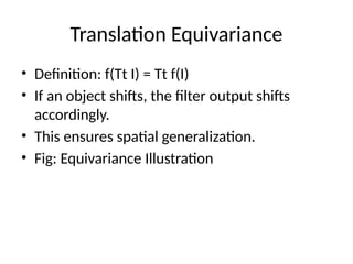
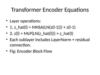
10. Vision Transformer (ViT) Overview
• ViT splits image into non-overlapping patches
and applies self-attention.
• No convolutions used.
• Each patch (P x P) flattened and embedded
into D-dimensional space.
• Fig: Patch Embedding Process

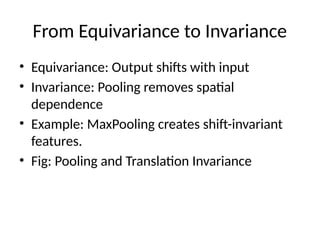
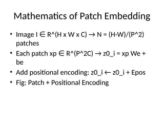
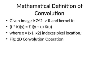
11. Mathematics of Patch Embedding
• Image I R^(H x W x C) → N = (H·W)/(P^2)
∈
patches
• Each patch xp R^(P^2C) → z0_i = xp We +
∈
be
• Add positional encoding: z0_i ← z0_i + Epos
• Fig: Patch + Positional Encoding

12. Transformer Encoder Equations
• Layer operations:
• 1. z_hat(l) = MHSA(LN(z(l-1))) + z(l-1)
• 2. z(l) = MLP(LN(z_hat(l))) + z_hat(l)
• Each sublayer includes LayerNorm + residual
connection.
• Fig: Encoder Block Flow

13. Multi-Head Self-Attention (MHSA)
• Attention(Q,K,V) = softmax(QK^T / sqrt(dk)) V
• Where Q = XWQ, K = XWK, V = XWV
• Captures global dependencies.
• Fig: Self-Attention Mechanism

14. Feed-Forward Network (MLP)
• MLP(x) = W2 * σ(W1x + b1) + b2
• Usually expansion ratio = 4.
• Activation: GELU(x) = 0.5x(1 + tanh(√(2/π)(x +
0.0447x^3)))
• Fig: Transformer MLP Block

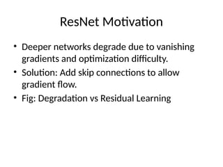
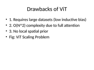
15. Drawbacks of ViT
• 1. Requires large datasets (low inductive bias)
• 2. O(N^2) complexity due to full attention
• 3. No local spatial prior
• Fig: ViT Scaling Problem

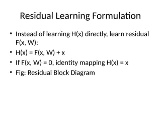
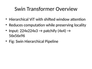
16. Swin Transformer Overview
• Hierarchical ViT with shifted window attention
• Reduces computation while preserving locality
• Input: 224x224x3 → patchify (4x4) →
56x56x96
• Fig: Swin Hierarchical Pipeline

17. Window-based Self-Attention
• Local attention on 7x7 windows → 49 tokens
per window
• Attention(Q,K,V) = softmax(QK^T / sqrt(d)) V
• FLOPs per window ≈ 2 * Nw^2 * d
• Fig: Window Attention Computation

18. FLOPs Comparison
• Global ViT: O(N^2) = 6.3x10^8
• Swin: Local windows O(M^2N) = 2.9x10^7
• ~20x reduction in computation.
• Fig: FLOPs Reduction Visualization

19. Shifted Windows
• Shift by (M/2, M/2) patches for cross-window
info.
• Enables overlapping receptive fields.
• Fig: Shifted vs Non-Shifted Windows

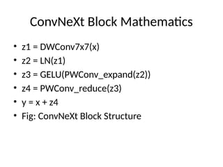
20. ConvNeXt Introduction
• Modernized CNN reintroducing convolutional
inductive biases with Transformer inspiration.
• Overcomes ViT limitations with efficient
convolutions.
• Fig: ConvNeXt Overview

21. ConvNeXt Block Mathematics
• z1 = DWConv7x7(x)
• z2 = LN(z1)
• z3 = GELU(PWConv_expand(z2))
• z4 = PWConv_reduce(z3)
• y = x + z4
• Fig: ConvNeXt Block Structure

22. FLOPs in ConvNeXt
• Example: H=W=28, C=192
• DWConv7x7 ≈ 7.4M
• Expand 1x1 Conv ≈ 116M
• Reduce 1x1 Conv ≈ 116M
• Total ≈ 239M FLOPs per block
• Fig: FLOP Breakdown

23. ConvNeXt vs Transformer
• DWConv ≈ Local Attention
• Inverted Bottleneck ≈ MLP Expansion
• LN + GELU → Transformer-style training
• ConvNeXt retains locality with efficiency.
• Fig: Comparison Table

24. Conclusion
• ConvNeXt bridges CNNs and Transformers:
• ConvNeXt = Modern ConvNet + Transformer-
inspired Design
• Efficient, robust, and hardware-friendly.
• Fig: Unified CNN-Transformer Paradigm