Recently, the use of artificial intelligence techniques has become widespread, having been adopted in brain-computer interfaces (BCIs) with electroencephalograms (EEGs). BCIs allow direct communication between a person's brain and a computer, and have various uses ranging from assistive technology to neuroscientific study. This paper provides an introductory overview of BCIs and EEG. We adopted the use of machine learning (ML) algorithms, including K-nearest neighbors (KNN), logistic regression, decision trees, random forests, and support vector machine (SVM). Additionally, we proposed a hybrid model of deep learning (DL) and ML by combining convolutional neural networks (CNNs) and SVMs. Our achieved 98% accuracy. The goal is to classify EEG signals into three emotional states: happy, normal, and sad. The study aims to achieve a comprehensive understanding of the effectiveness of these algorithms in accurately classifying emotional states based on EEG data. By comparing the performance of traditional ML methods and the proposed hybrid model, we seek to identify the most robust and accurate approach to sentiment classification.

1. IAES International Journal of Artificial Intelligence (IJ-AI)
Vol. 13, No. 3, September 2024, pp. 3671~3685
ISSN: 2252-8938, DOI: 10.11591/ijai.v13.i3.pp3671-3685  3671
Journal homepage: http://ijai.iaescore.com
Comparing emotion classification: machine learning algorithms
and hybrid model with support vector machines
Ghufran Hamid Zghair, Dheyaa Shaheed Al-Azzawi
Department of Software Science, College of Computer Science and Information Technology, Wasit University, Wasit, Iraq
Article Info ABSTRACT
Article history:
Received Jan 31, 2024
Revised Feb 12, 2024
Accepted Feb 28, 2024
Recently, the use of artificial intelligence techniques has become widespread,
having been adopted in brain-computer interfaces (BCIs) with
electroencephalograms (EEGs). BCIs allow direct communication between a
person's brain and a computer, and have various uses ranging from assistive
technology to neuroscientific study. This paper provides an introductory
overview of BCIs and EEG. We adopted the use of machine learning (ML)
algorithms, including K-nearest neighbors (KNN), logistic regression,
decision trees, random forests, and support vector machine (SVM).
Additionally, we proposed a hybrid model of deep learning (DL) and ML by
combining convolutional neural networks (CNNs) and SVMs. Our achieved
98% accuracy. The goal is to classify EEG signals into three emotional states:
happy, normal, and sad. The study aims to achieve a comprehensive
understanding of the effectiveness of these algorithms in accurately
classifying emotional states based on EEG data. By comparing the
performance of traditional ML methods and the proposed hybrid model, we
seek to identify the most robust and accurate approach to sentiment
classification.
Keywords:
Brain-computer interfaces
CNNs with SVMs
Deep learning
Electroencephalogram
Machine learning
This is an open access article under the CC BY-SA license.
Corresponding Author:
Ghufran Hamid Zghair
Department of Software Science, College of Computer Science and Information Technology, Wasit University
St. Textile, Al Kut, Wasit, Iraq
Email: ghufraan.hamed@uowasit.edu.iq
1. INTRODUCTION
The principle behind the brain-computer interface (BCI) is to establish a line of communication
between the human brain and a computer or other device. The BCI system monitors changes in brain activity
and computer screens or other real objects, such as emotions that have been categorised or other external
devices. For neurorehabilitation or as a support system for people with a variety of health problems or
long-term health effects, BCI has received substantial research in recent years. BCI technology can be effective
for idea-only communication [1], [2]. Machine learning (ML) algorithms use input data to achieve goals
without explicit programming, replicating human learning from experience [3], [4]. Deep learning (DL) is a
ML branch that uses artificial neural networks (ANNs) to create complex neural systems with over 10 layers.
It is crucial in medical image processing, disease classification, segmentation, and clinical data recognition [5],
[6]. Emotion is a multifaceted condition that reflects human consciousness, and is characterized as a response
to stimuli in the environment. Generally, emotions arise in response to thoughts, memories, or events within
our surroundings. They play a crucial role in decision-making and interpersonal communication among
humans. Decision-making is influenced by emotional states, and the presence of negative emotions can
contribute to both psychological and physical issues. Conversely, positive emotions may contribute to
improved health, whereas negative emotions could potentially result in a reduced quality of life [7]. In this

2.  ISSN: 2252-8938
Int J Artif Intell, Vol. 13, No. 3, September 2024: 3671-3685
3672
paper, we discuss a group of studies presented by researchers in the field of identifying emotions using different
algorithms and methods.
Djamal and Lodaya [8], emotional therapy, medical rehabilitation, and applications of the BCI all
depend on emotional identification. Electroencephalogram (EEG) signals fall into three categories: happy,
relaxed, and sad. This research suggests utilising wavelet and learning vector quantization (LVQ) to track
human emotion in real-time. Alpha, beta, and theta waves were created in 10 seconds by processing data from
480 sets of data. The method used wavelet extraction and an asymmetric channel to increase accuracy by 72%
to 87%. Without losing accuracy, LVQ reduced computation time to under a minute. For the purpose of
tracking emotional states in real time, a wireless EEG was integrated into the system. Reolid et al. [9] describes
an experiment to evaluate the emotional state categorization precision offered by the application programming
interface (API) of the emotiv EPOC+ headset. The international affective picture system (IAPS) dataset is used
in the study to examine the emotional states using photographs. To determine the classification accuracy,
participants' responses are compared to validated values, and ANNs are put to the test. The ANN setup with
three hidden layers and 30, 8, and 3 neurons for layers 1, 2, and 3 produces the best results. The emotional
states delivered by the headset can be employed in real-time applications based on users' emotional states with
high confidence thanks to this configuration's 85% classification accuracy. Additionally, the study shows that
multilayer perceptron ANN designs are enough.
Huang et al. [10] describes an EEG-based BCI system for emotion identification that uses
subject-specific frequency bands to identify happy and melancholy. It was verified in two studies and reached
an average online accuracy for two classes of 91.5%, with the gamma band being more closely associated with
emotions of happiness and melancholy. Ramdhani et al. [11], the BCI system model presented is based on
motor imagery and emotion. Eight classes are created from the recovered EEG signals using wavelet
transformation: "happy forward," "happy stop," "happy right," "happy left," "neutral forward," "neutral stop,"
"neutral right," and "neutral left". With AdaMax and VGG16, the model classified the characteristics into eight
groups with an accuracy of 90%. Users of this BCI system can control external devices without using their
muscles or motor abilities.
Ardito et al. [12], BCI allow for machine control using EEG signal processing. EEG signals were
used in a study to identify emotional states like valence, arousal, and dominance. The development of a deep
neural network to dynamically identify emotions led to the creation of a prototype for an EEG-based emotion
recognizer. As a result, the prototype can be used for screening and epidemiological research that require
real-time observation of emotional history. With a mean absolute error of 0.08 and an accuracy: R2
of 0.93, the
convolutional neural network (CNN) performed well. The high metrics, however, are based on a limited
population sample, necessitating additional validation on a larger test sample. Pandey and Sharma [13], the
BCI is a communication device for people with impairments and mental illnesses that translates commands
from brain EEG signals. A 96% accurate model for emotion classification developed recently in BCI
technology has the potential to enhance device performance.
Wu and Dai [14], the emo-net neural decoding framework, a data-driven method, aims to properly
read emotions from neural activity segments for emotional BCI. While DL has great potential, its development
has been hampered by the use of non-human primates and noise in training data. This method improves the
functionality and decoding skills of basic DL models, enabling the recognition of animal model emotion. DL
models are up to 92.02% accurate on a variety of classification and reconstruction tasks. Si et al. [15], a DL
model for emotion recognition utilising functional near-infrared spectroscopy (fNIRS) and videos is presented
in the study. the model achieves 90% outstanding decoding performance. The model also exhibits promise for
tasks requiring emotion recognition, although it has drawbacks, including the inability to subdivide emotions
and subpar decoding for negative versus neutral emotions.
Researchers who have explored the connection between EEG, BCIs, and emotion have made
significant contributions to the field. Their work has focused on investigating how EEG signals can be used to
detect and interpret emotional states in individuals using BCIs. These studies have shown promising results in
enabling communication and understanding of emotions in individuals with limited motor control. The
researchers have employed various methods, such as ML algorithms and pattern recognition techniques, to
analyse and classify EEG signals associated with different emotional states. In this research, we present a study
where we used some ML algorithms and proposed a hybrid model that combines DL with ML to achieve results
with acceptable accuracy and higher than others [8]‒[15]. We compared the results of the algorithms we
adopted in our study with each other, as well as with the results of other researchers.
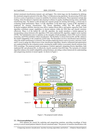
2. PROPOSAL MODEL SCHEMA
The proposed model for classifying emotions unfolds across five phases, offering a comprehensive
approach to leveraging EEG data. Phase1 of EEG dataset classification: the EEG dataset incorporates three

3. Int J Artif Intell ISSN: 2252-8938 
Comparing emotion classification: machine learning algorithms and hybrid … (Ghufran Hamid Zghair)
3673
distinct emotional classifications (natural, sad, and happy). This initial stage sets the foundation by defining
the emotional categories present in the data. Phase 2 of data processing operations: the processing of EEG data
involves a series of operations to ensure its suitability for emotion classification. These operations include data
loading, where the dataset is imported, data cleaning to enhance its quality, handling missing values, and finally
transforming data. The dataset is then divided into separate groups for training and testing, a critical step in
evaluating model performance. Phase 3 of ML algorithms: in the third stage, a group of ML algorithms is
employed for emotion classification. The chosen algorithms within this ML group include
K-nearest neighbors (KNNs), decision trees (DTs), random forests (RFs), and logistic regression (LR). Each
algorithm contributes unique capabilities to discern patterns within the EEG data and classify emotions
effectively. Phase 4 of the hybrid DL with ML algorithm: the model introduces a hybrid approach by
incorporating a choice between a DL algorithm, CNN, and a traditional ML algorithm, support vector machine
(SVM). This hybridization aims to capitalise on the strengths of both paradigms, where CNN excels in feature
extraction, and SVM contributes robust classification. The flexibility to choose between DL and ML enhances
the model's adaptability to the complexity of EEG data. The final phase involves classification and evaluation,
where the model's performance is assessed. This includes employing metrics such as accuracy, precision, recall,
and F1-score to gauge the effectiveness of the classification algorithms. Iterative refinement and optimization
are conducted based on the evaluation results, ensuring the model's ability to accurately classify emotions from
EEG recordings. The proposed model encompasses a holistic approach, integrating diverse algorithms, both
traditional ML and advanced DL, to effectively classify emotions from EEG data. The inclusion of a hybrid
algorithm enhances the model's adaptability and performance, providing a robust framework for understanding
and categorizing emotions in neural signals. As shown in Figure 1.
Figure 1. The proposal model schema
2.1. Electroencephalogram
EEG datasets are crucial for exploring and categorizing emotions, providing recordings of brain
activity to unveil neural patterns linked to diverse emotional states. The process of emotion classification with
Start
Dataset EEG (BCIs)
Dataset EEG split into two sets
Data loading
Data cleaning
Missing values
Transform data
Pre-processing
Training of 80% dataset Testing of 20% dataset
Classification Evaluation
CNN + SVM
DT
KNN RF
Logistic regression
Hybrid DL and ML Machine learning
RMSE
MSE F1-score
Precision
Recall
Accuracy
End
Feuture
Extraction
Section 2.1
Section 2.2
Section 2.4
Section 2.5
Section 2.3

4.  ISSN: 2252-8938
Int J Artif Intell, Vol. 13, No. 3, September 2024: 3671-3685
3674
EEG entails extracting significant features from these recordings, which then serve as inputs for ML models.
These datasets play a pivotal role in the creation and assessment of a wide range of algorithms, spanning from
classical approaches like LR and DT to sophisticated methods such as CNN and hybrid models. This
contributes to a deeper comprehension of emotions through neural signals [16].
2.2. Pre-processing
In the preparation phase for emotion classification using EEG datasets, crucial measures are taken to
enhance data quality before utilizing ML algorithms. This encompasses addressing missing values, converting
labels into numeric form, and choosing pertinent features. Ensuring uniform scaling through standardization
or naturalization is key, and the division of data into training and test sets is fundamental. Supplementary
techniques, such as feature scaling and transformation, are employed to optimize the performance of ensuing
emotion classification algorithms, thereby improving accuracy and dependability in identifying emotional
states [17]. Algorithm 1 representation of the steps performed in the code:
Algorithm 1. The phases of pre-processing and dividing the dataset
Input: Dataset
Output: Number of Missing Values, Transformed Data (X and Y), Scaled Data, Train-Test Split,
Standardized Features
Step 1: Start
Step 2: Import necessary libraries: (numpy, pandas, confusion_matrix, matplotlib. pyplot, seaborn,
accuracy_score, recall_score, roc_auc_score, classification_report, precision_score, f1_score,
mean_squared_error).
Step 3: Finding Number of Missing Values: a) Apply a function to check for missing values in each column
of the dataset. b) Display the shape of the dataset (data), indicating the number of rows and
columns.
Step 4: Transform Data: a) Define a function named 'Transform_data' taking 'data' as input. b) Replace
labels ('POSITIVE', 'NEUTRAL', 'NEGATIVE') in the 'label' column with numerical values (2, 0,
1). c) Separate the predictor variables (X) and the target variable (Y). d) Return X and Y.
Step 5: Call Transformation Function and Split Data: a) Call 'Transform_data(data)' to obtain X and Y. b)
Use 'MinMaxScaler' from 'sklearn. preprocessing' to scale the features in the range [0, 1].
Step 6: Train-Test Split: a) Import 'train_test_split' from 'sklearn. model_selection'. b) Split the dataset into
training and test sets (X_train, X_test, Y_train, Y_test) with a testing size of 20% and a training
size of 80%.
Step 7: Standardize Features: a) Import 'StandardScaler' from 'sklearn. preprocessing'. b) Standardize the
features using 'fit_transform' for training data and 'transform' for test data.
Step 8: End
2.3. Machine learning
ML algorithms use input data to achieve goals without explicit programming, replicating human
learning from experience. Used to analyze large datasets, perform predictive analytics faster than humans, and
use statistical theory to build mathematical models. This branch of artificial intelligence focuses on algorithm
development and assessment [18].
2.3.1. K-nearest neighbors
Utilized in emotion classification within EEG datasets, the KNN classifier algorithm determines the
emotion class of a data point by assessing the classes of its nearest neighbors. The approach relies on the
proximity of instances in feature space, assigning the most prevalent emotion within the KNN [19].
Well-suited for multiclass emotion classification, this method offers a straightforward yet efficient means of
identifying emotional states in EEG data, analyzing patterns based on neighboring instances in the dataset [20],
[21]. As shown in Figure 2. Algorithm 2 representation of the steps performed in the code:
Algorithm 2. Implementing the K-nearest neighbors algorithm
Input: Training Data (X_train, Y_train), Test Data (X_test)
Output: Trained Model, Predictions, Performance Metrics, Confusion Matrix, Classification Report, Error
Handling
Step 1: Start

5. Int J Artif Intell ISSN: 2252-8938 
Comparing emotion classification: machine learning algorithms and hybrid … (Ghufran Hamid Zghair)
3675
Step 2: Import necessary libraries: a) Import 'KNeighborsClassifier' from 'sklearn.neighbors'. b) Import
'model_selection' and 'neighbors' from 'sklearn'. c) Import other required libraries such as
(''accuracy_score, precision_score, recall_score, f1_score, mean_squared_error,
confusion_matrix'', classification_report, numpy, matplotlib. pyplot, and seaborn).
Step 3: Create a KNeighborsClassifier: Initialize a KNeighborsClassifier object as 'clf'.
Step 4: Train the classifier: Fit the classifier on the train-ing data (X_train and Y_train) and store the trained
model in 'knn_clf'.
Step 5: Predict outcomes for the test set: Use the train-ed classifier to predict outcomes for the test set
(`X_test`) and store the predictions in 'Y_pred_test'.
Step 6: Predict outcomes for the training set: Use the trained classifier to predict outcomes for the training
set ('X_train') and store the predictions in 'Y_pred_train'.
Step 7: Calculate and print performance metrics for the training and testing set: Calculate and print the
(''accuracy, precision, recall, F1-Score, mean squared error, and root mean squared error'').
Step 8: Generate and display a confusion matrix for the test set: a) Use 'confusion_matrix' to calculate the
confusion matrix for the test set. b) Create a heatmap using 'seaborn' and 'matplotlib.pyplot' to
visualize the confusion matrix.
Step 9: Print the classification report for the test set: Generate and print the classification report using
'classification_report' for the test set.
Step 10: End
Figure 2. Basic KNN structure
2.3.2. Logistic regression
LR, commonly utilized in emotion classification within EEG datasets, establishes a connection
between input features and emotions. It generates probabilities for each emotion class through a logistic
function, facilitating the prediction of the most probable emotion. This algorithm proves effective for both
binary and multiclass classification, offering valuable insights into discerning emotions from EEG data. Its
efficiency and interpretability contribute to a better understanding of the intricate patterns underlying emotional
states in EEG recordings [22], [23]. As shown in Figure 3. Algorithm 3 representation of the steps performed
in the code:
Algorithm 3. Implementing the logistic regression algorithm
Input: Training Data (X_train, Y_train), Test Data (X_test)
Output: Trained Model, Predictions, Performance Metrics, Confusion Matrix, Classification Report, Error
Handling
Step 1: Start
Step 2: Import necessary libraries: a) Import 'LogisticRegression' from 'sklearn. linear_model'. b) Import
other required libraries such as (''accuracy_score, precision_score, recall_score, f1_score,
mean_squared_error, confusion_matrix'', classification_report, numpy, matplotlib. pyplot, and
seaborn).
Step 3: Create a Logistic Regression model: Initialize a Logistic Regression model object as 'model'.
Step 4: Train the model: Fit the model on the training data (X_train and Y_train).
Step 5: Predict outcomes for the test set: Use the trained model to predict outcomes for the test set (X_test)
and store the predictions in 'y_pred_test'.
Step 6: Predict outcomes for the training set: Use the trained model to predict outcomes for the training set
(X_train) and store the predictions in 'Y_pred_train'.

6.  ISSN: 2252-8938
Int J Artif Intell, Vol. 13, No. 3, September 2024: 3671-3685
3676
Step 7: Calculate and print performance metrics for the training and testing set: Calculate and print the
(''accuracy, precision, recall, F1-Score, mean squared error, and root mean squared error'').
Step 8: Generate and display a confusion-matrix for the test set: a) Use 'confusion_matrix' to calculate the
confusion-matrix for the test set. b) Create a heatmap using 'seaborn' and 'matplotlib. pyplot' to
visualize the confusion matrix.
Step 9: Print the classification report for the test set: Generate and print the classification report using
'classification_report' for the test set.
Step 10: Handle potential errors during the generation of the confusion-matrix for the test set: Use a 'try-
except' block to catch any 'ValueError' during the generation of the confusion matrix and print an
error message if it occurs.
Step 11: End
Figure 3. Basic LR structure
2.3.3. Decision tree
Utilized in classifying emotions within EEG datasets, the DT classifier employs a tree-like model to
make decisions based on input features, forming a hierarchical structure of nodes [24]. Through recursive
partitioning, the dataset branches into nodes that culminate in leaf nodes, each representing specific emotion
classes. Particularly effective for multiclass emotion classification in EEG data, DT offer interpretable
outcomes by visualizing decision-making processes. They excel at identifying patterns associated with diverse
emotional states, contributing to insightful analyses in emotion classification [25]. As shown in Figure 4.
Algorithm 4 representation of the steps performed in the code:
Algorithm 4. Implementing the decision tree algorithm
Input: Training Data (X_train, Y_train), Test Data (X_test)
Output: Trained Model, Predictions, Performance Metrics, Confusion Matrix, Classification Report, Error
Handling
Step 1: Start
Step 2: Import necessary libraries: a) Import 'DecisionTreeClassifier' from 'sklearn. tree'. b) Import other
required libraries such as (''accuracy_score, precision_score, recall_score, f1_score,
mean_squared_error, confusion_matrix'', classification_report, numpy, matplotlib. pyplot, and
seaborn).
Step 3: Create a Decision Tree Classifier: Initialize a Decision Tree Classifier object as 'dtc_clf' with a
specified 'random_state'.
Step 4: Train the Decision Tree Classifier: Fit the Decision Tree Classifier on the training data (X_train
and Y_train).
Step 5: Predict outcomes for the test set: Use the train-ed Decision Tree Classifier to predict outcomes for
the test set (X_test) and store the predictions in 'y_pred_test'.
Step 6: Predict outcomes for the training set: Use the trained Decision Tree Classifier to predict outcomes
for the training set (X_train) and store the predictions in 'y_pred_train'.
Step 7: Calculate and print performance metrics for the training and testing set: Calculate and print the
(''accuracy, precision, recall, F1-Score, mean squared error, and root mean squared error'').
Step 8: Generate and display a confusion-matrix for the test set: a) Use 'confusion_matrix' to calculate the
confusion matrix for the test set. b) Create a heatmap using 'seaborn' and 'matplotlib. pyplot' to
visualize the confusion matrix.

7. Int J Artif Intell ISSN: 2252-8938 
Comparing emotion classification: machine learning algorithms and hybrid … (Ghufran Hamid Zghair)
3677
Step 9: Print the classification report for the test set: Generate and print the classification report using
'classification_report' for the test set.
Step 10: Handle potential errors during the generation of the confusion-matrix for the test set: Use a 'try-
except' block to catch any 'ValueError' during the generation of the confusion matrix and print an
error message if it occurs.
Step 11: End
Figure 4. Structure of the DT algorithm
2.3.4. Random forest
The RF classifier plays a vital role in emotion classification within EEG datasets. This ensemble
learning technique utilizes multiple DT to improve accuracy and resilience [26]. By consolidating predictions
from diverse trees, the RF mitigates overfitting, yielding more dependable outcomes. Particularly adept at
capturing intricate patterns in EEG data related to emotions, this algorithm's versatility, capacity for handling
multiclass scenarios, and resistance to noise render it an invaluable asset for identifying emotional states in
EEG recordings [1]. As shown in Figure 5. Algorithm 5 representation of the steps performed in the code:
Algorithm 5. Implementing the random forest algorithm
Input: Training Data (X_train, Y_train), Test Data (X_test)
Output: Trained Model, Predictions, Performance Metrics, Confusion Matrix, Classification Report, Error
Handling
Step 1: Start
Step 2: Import necessary libraries: a) Import 'RandomForestClassifier' from 'sklearn. ensemble'. b) Import
other required libraries such as (''accuracy_score, precision_score, recall_score, f1_score,
mean_squared_error, confusion_matrix'', classification_report, numpy, matplotlib. pyplot, and
seaborn).
Step 3: Create a Random Forest Classifier: a) Initialize a Random Forest Classifier object (rmf) with a
specified 'random_state'. b) Fit the Random Forest Classifier on the training data (X_train and
Y_train) and store the trained model in 'rmf_clf'.
Step 4: Predict outcomes for the test set: Use the trained Random Forest Classifier to predict outcomes for
the test set (X_test) and store the predictions in 'y_pred_test'.
Step 5: Predict outcomes for the training set: Use the trained Random Forest Classifier to predict outcomes
for the training set (X_train) and store the predictions in 'y_pred_train'.
Step 6: Calculate and print performance metrics for the training and testing set: Calculate and print the
(''accuracy, precision, recall, F1-Score, mean squared error, and root mean squared error'').
Step 7: Generate and display a confusion matrix for the test set: a) Use 'confusion_matrix' to calculate the
confusion matrix for the test set. b) Create a heatmap using 'seaborn' and 'matplotlib. pyplot' to
visualize the confusion matrix.
Step 8: Print the classification report for the test set: Generate and print the classification report using
'classification_report' for the test set.
Step 9: Handle potential errors during the generation of the confusion matrix for the test set: Use a 'try-
except' block to catch any 'ValueError' during the generation of the confusion matrix and print an
error message if it occurs.
Step 10: End

8.  ISSN: 2252-8938
Int J Artif Intell, Vol. 13, No. 3, September 2024: 3671-3685
3678
Figure 5. RF algorithm with n DT
2.4. Hybrid deep learning with machine learning
The integration of DL with ML is utilized for emotion classification in EEG datasets [27]. This hybrid
model combines DL architectures, including CNNs and SVMs, with traditional ML methods to optimize
performance. By synergistically leveraging the strengths of both paradigms, the model proficiently captures
spatial and temporal patterns within EEG data, ensuring resilient emotion recognition. This unified approach
significantly improves classification accuracy and adaptability, establishing it as a potent tool for deciphering
emotions in intricate EEG recordings [18].
2.4.1 Hybrid convolutional neural network with support vector machine
The fusion of a CNN with SVM classifier is utilized to classify emotions in EEG datasets [28]. This
hybrid method merges CNN's feature extraction capabilities with SVM's classification strength. CNN extracts
spatial features from EEG data, and SVM categorizes these features into emotions. This combined model
proficiently captures spatial and temporal patterns, boosting the precision of emotion classification in EEG
recordings, particularly in scenarios involving intricate and high-dimensional data [29]. As shown in Figure 6.
Algorithm 6 representation of the steps performed in the code:
Algorithm 6. Implementing the hybrid convolutional neural network with support vector machine algorithms
Input: Training and Testing Data (X_train, X_test, Y_train), Original Labels (Y_train), Parameters
Output: Trained Models (CNN, SVM), Predictions (CNN (Y_pred_cnn), SVM (Y_pred_svm)),
Performance Metrics (Accuracy, Classification Report, Additional Metrics), Visualizations
(Training History Plot, Confusion Matrix Plot)
Step 1: Start
Step 2: Import necessary libraries: a) Import 'pandas' as 'pd'. b) Import 'train_test_split' from 'sklearn.
Model _selection'. c) Import 'StandardScaler' from 'sklearn. preprocessing'. d) Import necessary
modules from 'keras': "Sequential, Dense, Conv1D, Flatten, and MaxPooling1D". e) Import 'SVC'
from 'sklearn.svm'. f) Import 'accuracy_score' and 'classification_report' from 'sklearn. Metrics '. k)
Import 'numpy' as 'np'.
Step 3: Reshape data for CNN: a) Reshape the training and testing data for 1D Convolutional Neural
Network (CNN) using 'reshape'. b) Assuming it's EEG data, reshape to (number_of_samples,
time_steps, 1).
Step 4: One-hot encode the labels: Use 'to_categorical' from 'tensorflow. keras. utils ' to convert the
categorical labels (Y_train and Y_test) to one-hot encoded format.
Step 5: Define the 1D CNN model: a) Initialize a sequential model (`cnn_model`). b) Add a 1D
convolutional layer with 64 filters, kernel size 3, and ReLU activation. c) Add a 1D MaxPooling
layer with pool size 2. d) Flatten the output. e) Add a dense layer with 50 units and ReLU activation.
e) Add the output layer with 3 units (for 3 classes) and softmax activation.
Step 6: Compile the model: Compile the model use-ing 'adam' optimizer and 'categorical_crossentropy'
loss.
Step 7: Train the model with one-hot encoded labels: a) Train the model on the reshaped training data
(X_train_cnn) with one-hot encoded labels (Y_train_one_hot). b) Use 10 epochs and a batch size
of 32.
Step 8: Plot training history: a) Create a DataFrame (histdf) from the training history. b) Plot training
accuracy and loss using 'matplotlib'.

9. Int J Artif Intell ISSN: 2252-8938 
Comparing emotion classification: machine learning algorithms and hybrid … (Ghufran Hamid Zghair)
3679
Step 9: Extract features from the trained CNN: Use the trained CNN model to extract features from the
reshaped training and test data.
Step 10: Train an SVM on the extracted features: a) Initialize an SVM model (svm_model) with a linear
kernel. b) Fit the SVM model on the extracted features and the original training labels.
Step 11: Make predictions with the SVM: Use the trained SVM model to make predictions on the extracted
features from the test set.
Step 12: Evaluate the model: a) Calculate and print accuracy. b) Print classification report.
Step 13: Calculate additional evaluation metrics: a) Calculate and print ''precision, recall, f1-score, mean
squared error, and root mean squared error''. b) Generate and display a confusion matrix using
'confusion_matrix' and 'seaborn'.
Step 14: End
Figure 6. The hybrid CNN with SVM
2.5. Classification and evaluation
In the realm of emotion classification with EEG datasets, the classification and evaluation process
entails utilizing diverse ML algorithms to categorize emotional states. Following model training with labeled
data, performance assessment utilizes metrics such as accuracy, precision, recall, and F1-score. This iterative
approach strives to enhance the model's proficiency in accurately discerning emotions. The incorporation of
robust evaluation measures ensures the credibility of emotion classification outcomes, fostering a more
profound comprehension of emotional states within EEG recordings [30].
3. RESULTS AND DISCUSSION
The results and discussion section presents the outcomes of the study which employed a combination of
algorithms, including ML and DL, to classify emotions using an EEG dataset. The algorithms processed the EEG
data, extracting patterns and features relevant to emotional states. ML algorithms were likely employed for their
ability to discern complex relationships within the data, while DL models, known for their capacity to
automatically learn hierarchical representations, played a crucial role in capturing intricate patterns. The results
showcase the effectiveness of the proposed approach in accurately categorizing emotions based on EEG signals.
Furthermore, the discussion interprets these findings, highlighting the significance of the chosen algorithms, their
performance metrics, and their potential implications for emotion recognition applications. This section
contributes to the overall understanding of the methodology's robustness and its implications for advancing
emotion classification in EEG-based studies. The following, we discuss several cases involving our findings.
3.1. Case studies of machine learning algorithms
The success of each system depends on its accuracy and performance. In this case, we discuss the
results of the ML algorithms for (KNN, LR, DT, and RF). Table 1 shows an explanation of the results we
reached in the training and testing phases. In which we used precision, recall, F1-score, mean squared error
(MSE), root mean squared error (RMSE), and accuracy to evaluate the models. The work of the proposed
system was divided into two phases: the first was training, and the second was testing with a total of 2132 data
sets. In the training phase, 80% of the total data was approved, as the algorithms achieved an accuracy of 98%,
88%, 100%, and 100% for each of the KNN, LR, DT, and RF algorithms for a data set of 1705. As for the
testing phase, 20% of the total data was used, as the algorithms achieved 94%, 88%, 94%, and 97% accuracy
for each of the KNN, LR, DT, and RF algorithms for a data set of 427.

10.  ISSN: 2252-8938
Int J Artif Intell, Vol. 13, No. 3, September 2024: 3671-3685
3680
Table 1. The accuracy results of ML algorithms (training and testing)
ML Precision Recall F1-Score MSE RMSE Accuracy Support
Training KNN 0.97 0.97 0.97 0.06 0.25 0.98 1705
LR 0.88 0.88 0.88 0.20 0.45 0.88
DT 1.00 1.00 1.00 0.00 0.00 1.00
RF 1.00 1.00 1.00 0.00 0.00 1.00
Testing KNN 0.94 0.94 0.94 0.11 0.32 0.94 427
LR 0.88 0.88 0.88 0.17 0.41 0.88
DT 0.94 0.94 0.94 0.11 0.33 0.94
RF 0.97 0.97 0.97 0.06 0.24 0.97
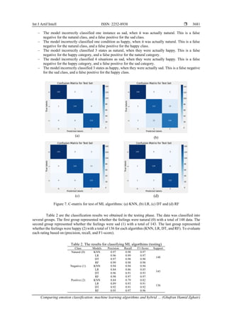
A confusion-matrix is a table that shows how well a classificat-ion model performs on a set of test
data, where the true labels are known. The rows represent the actual labels, and the columns represent the
expected labels. Each cell displays the number of cases that fall into the corresponding category. For example,
the cell in the upper left corner shows the number of cases that were correctly classified as natural, the cell in
the middle of the diagonal shows the number of cases that were correctly classified as wild, and the cell in the
lower right corner shows the number of cases that were correctly classified as happy. Cells outside the diagonal
show misclassifications, or instances that were expected to belong to a different category than the actual
category [31]. The following is a summary of the values in Figure 7.
a) Figure 7(a) C-matrix for test of KNN algorithm:
‒ The model naturally classified 145 cases as happy, 134 cases as sad, and 124 cases as happy. These are
the real positives of each category.
‒ The model incorrectly classified one instance as sad, when it was actually natural. This is a false
negative for the natural class, and a false positive for the sad class.
‒ The model incorrectly classified 4 cases as happy, when they were actually natural. This is a false
negative for the natural class, and a false positive for the happy class.
‒ The model incorrectly classified 3 states as natural , when they were actually happy. This is a false
negative for the happy category, and a false positive for the natural category.
‒ The model incorrectly classified 8 cases as sad, when they were actually happy. This is a false negative
for the happy category, and a false positive for the sad category.
‒ The model incorrectly classified 8 cases as happy, when they were actually sad. This is a false negative
for the sad class, and a false positive for the happy class.
b) Figure 7(b) C-matrix for test of LR algorithm:
‒ The model naturally classified 146 cases as happy, 123 cases as sad, and 108 cases as happy. These are
the real positives of each category.
‒ The model incorrectly classified one instance as sad, when it was actually natural. This is a false
negative for the natural class, and a false positive for the sad class.
‒ The model incorrectly classified 5 cases as happy, when they were actually natural. This is a false
negative for the natural class, and a false positive for the happy class.
‒ The model incorrectly classified 2 cases as natural, when they were actually happy. This is a false
negative for the happy category, and a false positive for the natural category.
‒ The model incorrectly classified 19 cases as sad, when they were actually happy. This is a false negative
for the happy category, and a false positive for the sad category.
‒ The model incorrectly classified 23 cases as happy, when they were actually sad. This is a false negative
for the sad class, and a false positive for the happy class.
c) Figure 7(c) C-matrix for test of DT algorithm:
‒ The model naturally classified 145 cases as happy, 130 cases as sad, and 126 cases as happy. These are
the real positives of each category.
‒ The model incorrectly classified 4 cases as happy, when they were actually natural. This is a false
negative for the natural class, and a false positive for the happy class.
‒ The model incorrectly classified 3 states as natural, when they were actually happy. This is a false
negative for the happy category, and a false positive for the natural category.
‒ The model incorrectly classified 13 cases as sad, when they were actually happy. This is a false negative
for the happy category, and a false positive for the sad category.
‒ The model incorrectly classified 6 states as happy, when they were actually sad. This is a false negative
for the sad class, and a false positive for the happy class.
d) Figure 7(d) C-matrix for test of RF algorithm:
‒ The model naturally classified 145 cases as happy, 138 cases as sad, and 132 cases as happy. These are
the real positives of each category.

11. Int J Artif Intell ISSN: 2252-8938 
Comparing emotion classification: machine learning algorithms and hybrid … (Ghufran Hamid Zghair)
3681
‒ The model incorrectly classified one instance as sad, when it was actually natural. This is a false
negative for the natural class, and a false positive for the sad class.
‒ The model incorrectly classified one condition as happy, when it was actually natural. This is a false
negative for the natural class, and a false positive for the happy class.
‒ The model incorrectly classified 3 states as natural, when they were actually happy. This is a false
negative for the happy category, and a false positive for the natural category.
‒ The model incorrectly classified 4 situations as sad, when they were actually happy. This is a false
negative for the happy category, and a false positive for the sad category.
‒ The model incorrectly classified 3 states as happy, when they were actually sad. This is a false negative
for the sad class, and a false positive for the happy class.
(a) (b)
(c) (d)
Figure 7. C-matrix for test of ML algorithms: (a) KNN, (b) LR, (c) DT and (d) RF
Table 2 are the classification results we obtained in the testing phase. The data was classified into
several groups. The first group represented whether the feelings were natural (0) with a total of 148 data. The
second group represented whether the feelings were sad (1) with a total of 143. The last group represented
whether the feelings were happy (2) with a total of 136 for each algorithm (KNN, LR, DT, and RF). To evaluate
each rating based on (precision, recall, and F1-score).
Table 2. The results for classifying ML algorthims (testing)
Class Models Precision Recall F1-Score Support
Natural (0) KNN 0.97 0.98 0.97
148
LR 0.96 0.99 0.97
DT 0.97 0.98 0.98
RF 0.99 0.98 0.98
Negative (1) KNN 0.94 0.94 0.94
143
LR 0.84 0.86 0.85
DT 0.96 0.91 0.93
RF 0.98 0.97 0.97
Positive (2) KNN 0.84 0.79 0.82
136
LR 0.89 0.93 0.91
DT 0.92 0.91 0.92
RF 0.95 0.97 0.96

12.  ISSN: 2252-8938
Int J Artif Intell, Vol. 13, No. 3, September 2024: 3671-3685
3682
3.2. Case studies of hybrid deep learning with machine learning algorithms
In this case, we discuss the results of the hybrid system our proposed. In which the CNN DL algorithm
was adopted to train and test the system with the SVM ML algorithm to classify the results into three groups
of emotions (natural, sad, and happy). Table 3 and Figure 8 show the training phase where we achieved 100%
accuracy and 0% loss. As shown in Figure 8, the loss index, which represents the orange line, decreased and
the accuracy index, which represents the blue line, increased after they reached Epoch 10/10.
A confusion matrix serves as a tabular representation for evaluating the performance of a classification
model on a specific set of test data with known true labels. It comprises rows representing actual labels and
columns indicating expected labels. Each cell indicates the count of cases falling into its corresponding
category. Correct classifications are depicted along the diagonal, with misclassifications shown in cells outside
the diagonal [31]. The provided summary encapsulates the key values outlined in Figure 9. Figure 9 C-matrix
for test of hybrid CNN with SVM algorithm:
‒ The model naturally classified 141 cases as happy, 146 cases as sad, and 133 cases as happy. These are the
real positives of each category.
‒ The model incorrectly classified 3 cases as happy, when they were actually natural. This is a false negative
for the natural class, and a false positive for the happy class.
‒ The model incorrectly classified 2 states as natural, when they were actually happy. This is a false negative
for the happy category, and a false positive for the natural category.
‒ The model incorrectly classified 2 cases as sad, when they were actually happy. This is a false negative for
the happy category, and a false positive for the sad category.
Table 3. The epochs for training the hybrid model
Epochs Loss Accuracy
Epoch 1/10 1.0059 0.8194
Epoch 2/10 0.1997 0.9390
Epoch 3/10 0.1460 0.9484
Epoch 4/10 0.0556 0.9865
Epoch 5/10 0.0430 0.9906
Epoch 6/10 0.0291 0.9930
Epoch 7/10 0.0186 0.9988
Epoch 8/10 0.0104 1.0000
Epoch 9/10 0.0078 1.0000
Epoch 10/10 0.0055 1.0000
Figure 8. The epochs for training the hybrid model
(CNN+SVM)
Figure 9. C-Matrix for test of hybrid CNN with
SVM algorithm
Table 4 shows the classification results our obtained in the testing phase. The data was classified into
several groups. The first group represented if the feelings were natural (0) with a total of 148, the second group
represented if the feelings were sad (1) with a total of 143, and the last group represented if the feelings were
happy (2) with a total of 136 for the proposed hybrid system in which our adopted the CNN with SVM
algorithm. The rating for each classification is calculated based on (precision, recall, F1-score, and accuracy).
In which we achieved 98% accuracy.
x
y

13. Int J Artif Intell ISSN: 2252-8938 
Comparing emotion classification: machine learning algorithms and hybrid … (Ghufran Hamid Zghair)
3683
Table 4. The results for classifying hybrid CNN with SVM algorithms (testing)
DL with ML – Models Class Precision Recall F1-Score Support
Hybrid CNN with
SVM Algorithm
Natural (0) 0.98 0.99 0.98 148
Negative (1) 1.00 0.99 0.99 143
Positive (2) 0.97 0.98 0.97 136
Accuracy 0.98 427
In Table 5, when comparing the results we achieved in the first case shown in section 3.1 with the
results our achieved in the second case in section 3.2, it turns out that the hybrid system is characterized by
higher accuracy in achieving results, as shown in Figure 10. Therefore, it is preferable to adopt a hybrid system
to achieve high accuracy in emotion classification. Also, in Table 6, we discuss the test results reached by a
group of researchers and compare them with the accuracy we achieved in the proposed hybrid system.
Table 6, shows the differences that show that the results achieved by our paper are 98% higher than the results
achieved by the researchers mentioned in Figure 11.
Table 5. Comparison of results ML with results DL+ML
AI Models Accuracy
ML
KNN 94%
LR 88%
DT 94%
RF 97%
DL+ML CNN + SVM 98%
Figure 10. The accuracy chart of our study results
Table 6. Comparison of our results with other researcher's results
Authors [8] [9] [10] [11] [12] [13] [14] [15] Our
Years 2017 2018 2019 2020 2022 2022 2023 2023 2024
Models Wavelet analysis
and LVQ
ANNs Real-time emotion
recognition system
CNN CNN-
1D
LGBM,
RFC, DTC
Emo-
Net
fNIRS CNN+SVM
Accuracy 87% 85% 91.5% 90% 93% 96% 92.02% 90% 98%
Figure 11. A chart of the accuracy of our study results with the researchers' results

14.  ISSN: 2252-8938
Int J Artif Intell, Vol. 13, No. 3, September 2024: 3671-3685
3684
4. CONCLUSION
Our research employed various ML algorithms (KNNs, LR, DT, and RF) for emotion classification
(94%, 88%, 94%, and 97%) and introduced a hybrid model combining DL (CNN) with ML (SVM). The
proposed hybrid system demonstrated exceptional performance, achieving an impressive 98% accuracy in
emotion classification. Comparative analysis against existing research highlighted the superior results of our
model, showcasing its efficacy in distinguishing emotions. This underscores the significance of hybrid
approaches in enhancing accuracy and reliability in emotion classification systems.
REFERENCES
[1] E. Antoniou et al., “EEG-based eye movement recognition using brain–computer interface and random forests,” Sensors, vol. 21,
no. 7, pp. 1–12, Mar. 2021, doi: 10.3390/s21072339.
[2] P. Stegman, C. S. Crawford, M. Andujar, A. Nijholt, and J. E. Gilbert, “Brain-computer interface software: A review and
discussion,” IEEE Transactions on Human-Machine Systems, vol. 50, no. 2, pp. 101–115, 2020, doi: 10.1109/THMS.2020.2968411.
[3] D. S. Al-Azzawi, “Evaluation of genetic algorithm optimization in machine learning,” Journal of Information Science and
Engineering, vol. 36, no. 2, pp. 231–241, 2020, doi: 10.6688/JISE.202003_36(2).0004.
[4] I. El Naqa and M. J. Murphy, “What is machine learning?,” in Machine Learning in Radiation Oncology, Cham: Springer
International Publishing, pp. 3–11, 2015, doi: 10.1007/978-3-319-18305-3_1.
[5] D. S. Al-Azzawi, “Application and evaluation of the neural network in gearbox,” Telecommunication Computing Electronics and
Control (TELKOMNIKA), vol. 18, no. 1, pp. 19–29, Feb. 2020, doi: 10.12928/telkomnika.v18i1.13760.
[6] A. S. Lundervold and A. Lundervold, “An overview of deep learning in medical imaging focusing on MRI,” Zeitschrift fur
Medizinische Physik, vol. 29, no. 2, pp. 102–127, 2019, doi: 10.1016/j.zemedi.2018.11.002.
[7] M. Naji, M. Firoozabadi, and P. Azadfallah, “Emotion classification during music listening from forehead biosignals,” Signal,
Image and Video Processing, vol. 9, no. 6, pp. 1365–1375, 2015, doi: 10.1007/s11760-013-0591-6.
[8] E. C. Djamal and P. Lodaya, “EEG based emotion monitoring using wavelet and learning vector quantization,” in 2017 4th
International Conference on Electrical Engineering, Computer Science and Informatics (EECSI), IEEE, Sep. 2017, pp. 1–6, doi:
10.1109/EECSI.2017.8239090.
[9] R. S. -Reolid et al., “Artificial neural networks to assess emotional states from brain-computer interface,” Electronics, vol. 7, no.
12, pp. 1–12, Dec. 2018, doi: 10.3390/electronics7120384.
[10] H. Huang et al., “An EEG-Bbased brain computer interface for emotion recognition and its application in patients with disorder of
consciousness,” IEEE Transactions on Affective Computing, vol. 12, no. 4, pp. 832–842, Oct. 2021, doi:
10.1109/TAFFC.2019.2901456.
[11] D. R. Ramdhani, E. C. Djamal, and F. Nugraha, “Brain-computer interface based on motor imagery and emotion using convolutional
neural networks,” in 2020 FORTEI-International Conference on Electrical Engineering (FORTEI-ICEE), IEEE, pp. 108–112, Sep.
2020, doi: 10.1109/FORTEI-ICEE50915.2020.9249937.
[12] C. Ardito et al., “Brain computer interface: deep learning approach to predict human emotion recognition,” in 2022 IEEE
International Conference on Systems, Man, and Cybernetics (SMC), IEEE, Oct. 2022, pp. 2689–2694, doi:
10.1109/SMC53654.2022.9945554.
[13] N. Pandey and O. Sharma, “Emotion recognition classification using an EEG-based brain computer interface system based on
different machine learning models,” in 2022 2nd International Conference on Innovative Sustainable Computational Technologies
(CISCT), IEEE, pp. 1–5, Dec. 2022, doi: 10.1109/CISCT55310.2022.10046601.
[14] X. Wu and J. Dai, “A deep-learning-based neural decoding framework for emotional brain-computer interfaces,” ArXiv-Computer
Science, pp. 1–22, 2023.
[15] X. Si, H. He, J. Yu, and D. Ming, “Cross-subject emotion recognition brain–computer interface based on fNIRS and DBJNet,”
Cyborg and Bionic Systems, vol. 4, Jan. 2023, doi: 10.34133/cbsystems.0045.
[16] E. P. Torres P., E. A. Torres, M. H. -Álvarez, and S. G. Yoo, “EEG-based BCI emotion recognition: A survey,” Sensors, vol. 20,
no. 18, pp. 1–36, 2020, doi: 10.3390/s20185083.
[17] S. García, J. Luengo, and F. Herrera, “Data preprocessing in data mining,” Intelligent Systems Reference Library, vol. 72, 2015.
[18] S. Raschka and V. Mirjalili, “Python machine learning: machine learning and deep learning with python: scikit-Learn, and
TensorFlow,” Birmingham: PACKT Publishing, 2019.
[19] D. S. Al-Azzawy and F. M. L. Al-Rufaye, “Arabic words clustering by using K-means algorithm,” 2017 Annual Conference on
New Trends in Information and Communications Technology Applications, NTICT 2017, pp. 263–267, 2017, doi:
10.1109/NTICT.2017.7976098.
[20] “k ‐Nearest Neighbor Algorithm,” in Discovering Knowledge in Data, Wiley, pp. 149–164, 2014, doi: 10.1002/9781118874059.ch7.
[21] Z. Min-Ling and Z. Zhi-Hua, “ML-KNN: a lazy learning approach to multi-label learning,” Pattern recognition, vol. 40, no. 7, pp.
2038–2048, 2007.
[22] A. Jacob, “Modelling speech emotion recognition using logistic regression and decision trees,” International Journal of Speech
Technology, vol. 20, no. 4, pp. 897–905, 2017, doi: 10.1007/s10772-017-9457-6.
[23] T. Rymarczyk, E. Kozłowski, G. Kłosowski, and K. Niderla, “Logistic regression for machine learning in process tomography,”
Sensors, vol. 19, no. 15, 2019, doi: 10.3390/s19153400.
[24] B. Charbuty and A. Abdulazeez, “Classification based on decision tree algorithm for machine learning,” Journal of Applied Science
and Technology Trends, vol. 2, no. 1, pp. 20–28, 2021, doi: 10.38094/jastt20165.
[25] R. Chalupnik, K. Bialas, Z. Majewska, and M. Kedziora, “Using simplified EEG-based brain computer interface and decision tree
classifier for emotions detection,” Lecture Notes in Networks and Systems, vol. 450 LNNS, pp. 306–316, 2022, doi: 10.1007/978-
3-030-99587-4_26.
[26] P. Palimkar, R. N. Shaw, and A. Ghosh, “Machine learning technique to prognosis diabetes disease: random forest classifier
approach,” Lecture Notes in Networks and Systems, vol. 218, pp. 219–244, 2022, doi: 10.1007/978-981-16-2164-2_19.
[27] M. Saeidi et al., “Neural decoding of eeg signals with machine learning: a systematic review,” Brain Sciences, vol. 11, no. 11, 2021,
doi: 10.3390/brainsci11111525.
[28] A. Saidi, S. B. Othman, and S. B. Saoud, “A novel epileptic seizure detection system using scalp EEG signals based on hybrid
CNN-SVM classifier,” IEEE Symposium on Industrial Electronics and Applications, ISIEA, 2021, doi:

15. Int J Artif Intell ISSN: 2252-8938 
Comparing emotion classification: machine learning algorithms and hybrid … (Ghufran Hamid Zghair)
3685
10.1109/ISIEA51897.2021.9510002.
[29] W. Gong et al., “A novel deep learning method for intelligent fault diagnosis of rotating machinery based on improved CNN-SVM
and multichannel data fusion,” Sensors, vol. 19, no. 7, 2019, doi: 10.3390/s19071693.
[30] B. Kaur, D. Singh, and P. P. Roy, “EEG based emotion classification mechanism in BCI,” Procedia Computer Science, vol. 132,
pp. 752–758, 2018, doi: 10.1016/j.procs.2018.05.087.
[31] M. Heydarian, T. E. Doyle, and R. Samavi, “MLCM: Multi-label confusion matrix,” IEEE Access, vol. 10, pp. 19083–19095, 2022,
doi: 10.1109/ACCESS.2022.3151048.
BIOGRAPHIES OF AUTHORS
Ghufran Hamid Zghair is M.Sc. student at the Department of Software Science,
College of Computer Science and Information Technology, Wasit University, Wasit, Iraq.
She is working on machine learning for brain-computer interfaces: decoding and
classification of neural signal. She can be contacted at email:
ghufraan.hamed@uowasit.edu.iq.
Dheyaa Shaheed Al-Azzawi is Ph.D. from the Iraqi Commission for Computers
and Informatics in Baghdad. He is currently a full professor at the Department of Software
Science, College of Computer Science and Information Technology, Wasit University, Wasit,
Iraq. His research interests include artificial intelligence, machine learning, and deep
learning. He can be contacted at email: dalazzawi@uowasit.edu.iq.