Downloaded 10 times


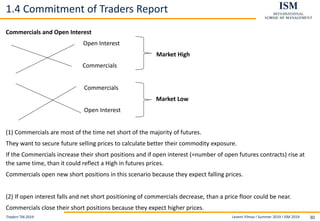
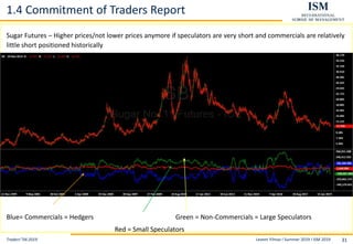
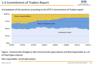
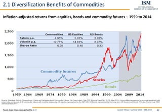


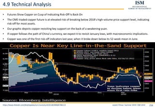
![Levent Yilmaz I Summer 2019 I ISM 2019 138
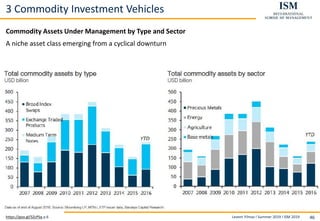
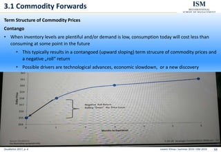
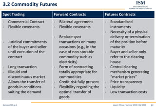
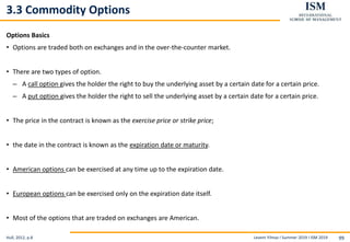
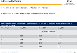
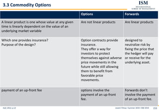
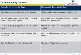
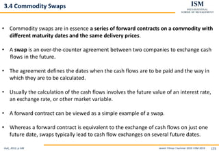
3.3 Commodity Options
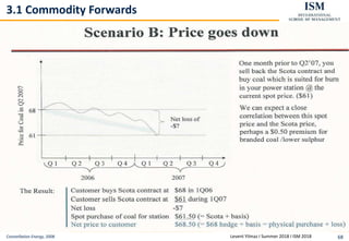
https://bit.ly/2DIxNs6
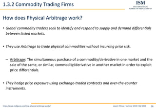
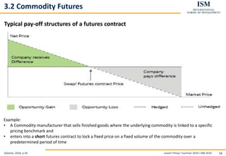
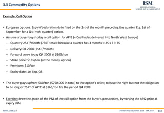
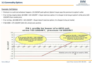
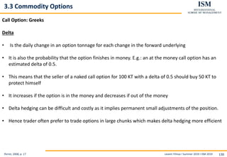
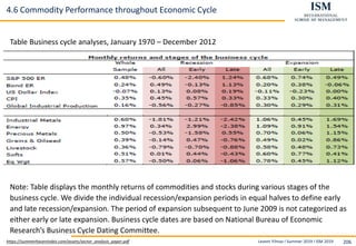
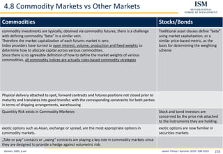
Example: Selling Option Strangle
• Selling the February crude 90 call, 45 put strangle for premiums of $600 per side.
• Margin per trade $1875.
• If worthless at expiration, the options would produce a 64% [(2 x 600 / 1875] return on investment.
• Strangle writers are NOT trying to predict what prices will do – only pick a price window where prices
will likely remain.
• Option strangles: offsetting nature (one side balancing out the other in an adverse move).
• By selling the option, the seller’s other risk is that the value of the option could increase during the
life of the option, thus increasing margin requirement to remain in the trade.
• The Option Seller wants to sell an option that is far enough out of the money and with low enough
volatility that the market can move a long way without greatly affecting the price or margin
requirement of her option.
• The strangle is most effective when the price of the underlying market remains in a defined range.
• While trending markets are not best for this approach, this does not mean that volatile markets
should be overlooked for strangling opportunities.
• Volatile markets often can still trade in wide trading ranges, and the volatility can boost option
premiums, meaning that a strangle often can be sold with a very wide profit zone.](https://image.slidesharecdn.com/ismfoliencommodityportfoliomanagement2019ss-5june2019acompressed-191105091803/85/Commodity-Portfolio-Management-138-320.jpg)


![Levent Yilmaz I Summer 2019 I ISM 2019 223
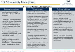
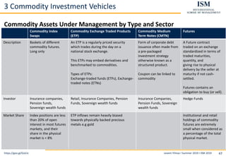
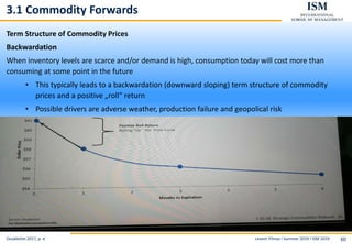
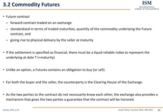
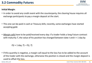
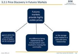
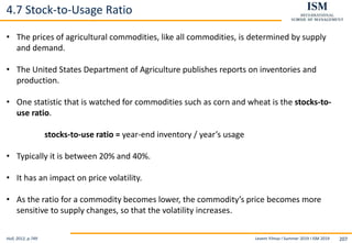
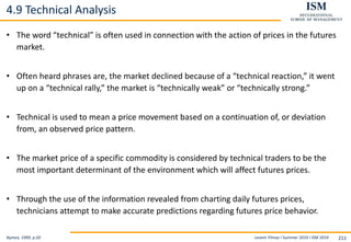
5.2 Overbought/Oversold Indicator
• The SG OBOS indicator defines and identifies “oversold” (“overbought”) commodities on a
weekly basis as those that are lying at the intersection of extremes in both short (long)
positioning and price weakness (strength).
• Commodities within the “oversold” (“overbought”) box are trading in the bottom (top)
25% of their price range and have a short (long) position (calculated as the short [long]
Money Manager [MM] open interest [OI] as a percentage of total OI) more than 75% of
the historical maximum.
• These commodities are vulnerable to short-covering (profit-taking).
https://goo.gl/Kk1WHU p.12](https://image.slidesharecdn.com/ismfoliencommodityportfoliomanagement2019ss-5june2019acompressed-191105091803/85/Commodity-Portfolio-Management-223-320.jpg)


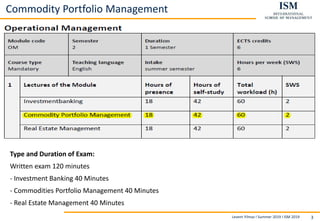
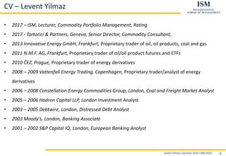
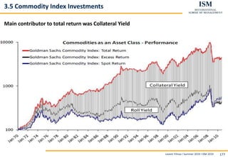
The document provides details about a course on Commodity Portfolio Management taught by Levent Yilmaz at ISM in the summer term of 2019, including the exam structure and Levent Yilmaz's CV. It also includes the content pages which lists the topics to be covered in the course such as commodity basics, drivers of commodity markets, and commodity portfolio management.


