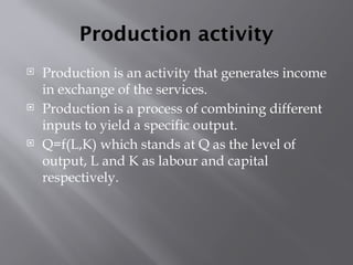
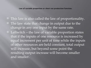
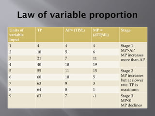
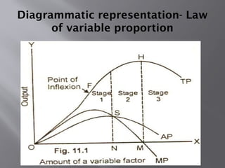
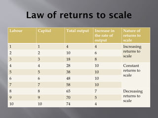
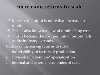
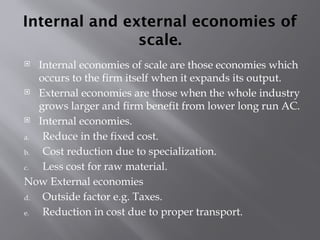
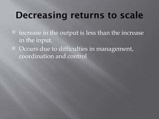
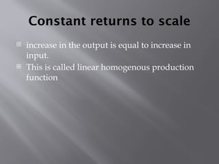
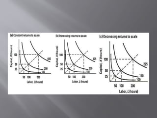
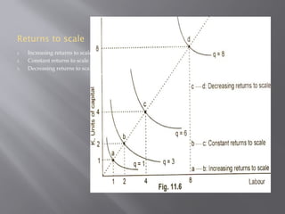
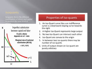
BUSINESS ECONOMICS AND
QUANTITATIVE TECHNIQUE
PAPER 3CH1
3RD
YEAR B.COM HONOURS.
Sandeep Sundas
Dept. of Economics
Kaliyaganj College
Production activity
 Production is an activity that generates income
in exchange of the services.
 Production is a process of combining different
inputs to yield a specific output.
 Q=f(L,K) which stands at Q as the level of
output, L and K as labour and capital
respectively.
Laws of production
 Law of variable proportion or short run
production function.
 Law of returns to scale or long run production
function.
Law of variable proportion or short run production function.
 This law is also called the law of proportionality.
 The law state that change in output due to the
change in any one input by the same rate.
 Leftwitch – the law of variable proportion states
that if the inputs of one resource is increased by
equal increment per unit of time while the inputs
of other resources are held constant, total output
will increase, but beyond some point the
resulting output increase will become smaller
and smaller.
Law of variable proportion
Units of
variable
input
TP AP= (TP/L) MP =
(dTP/dL)
Stage
1 4 4 4 Stage 1
MP>AP
MP increases
more than AP
2 10 5 6
3 21 7 11
4 40 10 19
5 55 11 15 Stage 2
MP increases
but at slower
rate. TP is
maximum
6 60 10 5
7 63 9 3
8 64 8 1
9 63 7 -1 Stage 3
MP<0
MP declines
Diagrammatic representation- Law
of variable proportion
Law of variable proportion-
Assumptions
 The law is based on no change in the
technology.
 All units of the variable factor are homogenous.
 Only one factor is variable, others remaining
constant.
 The products are measured in physical units.
Example quintals, tonnes etc.
 It is assumed that all variable factors are
equally efficient.
 Only applicable under short run.
Law of returns to scale
 In the long run all factors of production are variable.
The scale of production can be changed by changing
the quantity of all factors of production.
 Koutsoyiannis – the term returns to scale refers to the
changes in output as all factors change by the same
proportion.
 Leibhafsky – returns to scale relates to the behavior of
total output as all inputs are varied and is a long run
concept.
 The law states that change in output due to the change
in all the inputs by the same rate and same percentage.
Types of returns to scale
 Increasing returns to scale
 Decreasing return to scale
 Diminishing returns to scale.
Law of returns to scale
Labour Capital Total output Increase in
the rate of
output
Nature of
returns to
scale
1 1 4 4 Increasing
returns to
scale
2 2 10 6
3 3 18 8
4 4 28 10 Constant
returns to
scale
5 5 38 10
6 6 48 10
7 7 58 10
8 8 65 7 Decreasing
returns to
scale
9 9 70 5
10 10 74 4
Increasing returns to scale
 Increase in output is more than increase in
input.
 This is also known as law of diminishing costs.
 This is because the cost per unit of output falls
as the industry expands.
Causes of increasing returns to scale
a. Indivisibility of factors of production
b. Division of labour and specialization
c. Internal and external economies of scale.
Internal and external economies of
scale.
 Internal economies of scale are those economies which
occurs to the firm itself when it expands its output.
 External economies are those when the whole industry
grows larger and firm benefit from lower long run AC.
 Internal economies.
a. Reduce in the fixed cost.
b. Cost reduction due to specialization.
c. Less cost for raw material.
Now External economies
d. Outside factor e.g. Taxes.
e. Reduction in cost due to proper transport.
Decreasing returns to scale
 increase in the output is less than the increase
in the input.
 Occurs due to difficulties in management,
coordination and control
Constant returns to scale
 increase in the output is equal to increase in
input.
 This is called linear homogenous production
function
Returns to scale
1. Increasing returns to scale
2. Constant returns to scale
3. Decreasing returns to scale
Isoquants
Isoquants shows the different
combination of labour and capital
to produce the same level of
output.
Thank you

Commerce 3rd Year Hons_production activity1.pptx

  • 1.
    BUSINESS ECONOMICS AND QUANTITATIVETECHNIQUE PAPER 3CH1 3RD YEAR B.COM HONOURS. Sandeep Sundas Dept. of Economics Kaliyaganj College
  • 2.
    Production activity  Productionis an activity that generates income in exchange of the services.  Production is a process of combining different inputs to yield a specific output.  Q=f(L,K) which stands at Q as the level of output, L and K as labour and capital respectively.
  • 3.
    Laws of production Law of variable proportion or short run production function.  Law of returns to scale or long run production function.
  • 4.
    Law of variableproportion or short run production function.  This law is also called the law of proportionality.  The law state that change in output due to the change in any one input by the same rate.  Leftwitch – the law of variable proportion states that if the inputs of one resource is increased by equal increment per unit of time while the inputs of other resources are held constant, total output will increase, but beyond some point the resulting output increase will become smaller and smaller.
  • 5.
    Law of variableproportion Units of variable input TP AP= (TP/L) MP = (dTP/dL) Stage 1 4 4 4 Stage 1 MP>AP MP increases more than AP 2 10 5 6 3 21 7 11 4 40 10 19 5 55 11 15 Stage 2 MP increases but at slower rate. TP is maximum 6 60 10 5 7 63 9 3 8 64 8 1 9 63 7 -1 Stage 3 MP<0 MP declines
  • 6.
  • 7.
    Law of variableproportion- Assumptions  The law is based on no change in the technology.  All units of the variable factor are homogenous.  Only one factor is variable, others remaining constant.  The products are measured in physical units. Example quintals, tonnes etc.  It is assumed that all variable factors are equally efficient.  Only applicable under short run.
  • 8.
    Law of returnsto scale  In the long run all factors of production are variable. The scale of production can be changed by changing the quantity of all factors of production.  Koutsoyiannis – the term returns to scale refers to the changes in output as all factors change by the same proportion.  Leibhafsky – returns to scale relates to the behavior of total output as all inputs are varied and is a long run concept.  The law states that change in output due to the change in all the inputs by the same rate and same percentage.
  • 9.
    Types of returnsto scale  Increasing returns to scale  Decreasing return to scale  Diminishing returns to scale.
  • 10.
    Law of returnsto scale Labour Capital Total output Increase in the rate of output Nature of returns to scale 1 1 4 4 Increasing returns to scale 2 2 10 6 3 3 18 8 4 4 28 10 Constant returns to scale 5 5 38 10 6 6 48 10 7 7 58 10 8 8 65 7 Decreasing returns to scale 9 9 70 5 10 10 74 4
  • 11.
    Increasing returns toscale  Increase in output is more than increase in input.  This is also known as law of diminishing costs.  This is because the cost per unit of output falls as the industry expands. Causes of increasing returns to scale a. Indivisibility of factors of production b. Division of labour and specialization c. Internal and external economies of scale.
  • 12.
    Internal and externaleconomies of scale.  Internal economies of scale are those economies which occurs to the firm itself when it expands its output.  External economies are those when the whole industry grows larger and firm benefit from lower long run AC.  Internal economies. a. Reduce in the fixed cost. b. Cost reduction due to specialization. c. Less cost for raw material. Now External economies d. Outside factor e.g. Taxes. e. Reduction in cost due to proper transport.
  • 13.
    Decreasing returns toscale  increase in the output is less than the increase in the input.  Occurs due to difficulties in management, coordination and control
  • 14.
    Constant returns toscale  increase in the output is equal to increase in input.  This is called linear homogenous production function
  • 16.
    Returns to scale 1.Increasing returns to scale 2. Constant returns to scale 3. Decreasing returns to scale
  • 17.
    Isoquants Isoquants shows thedifferent combination of labour and capital to produce the same level of output.
  • 18.