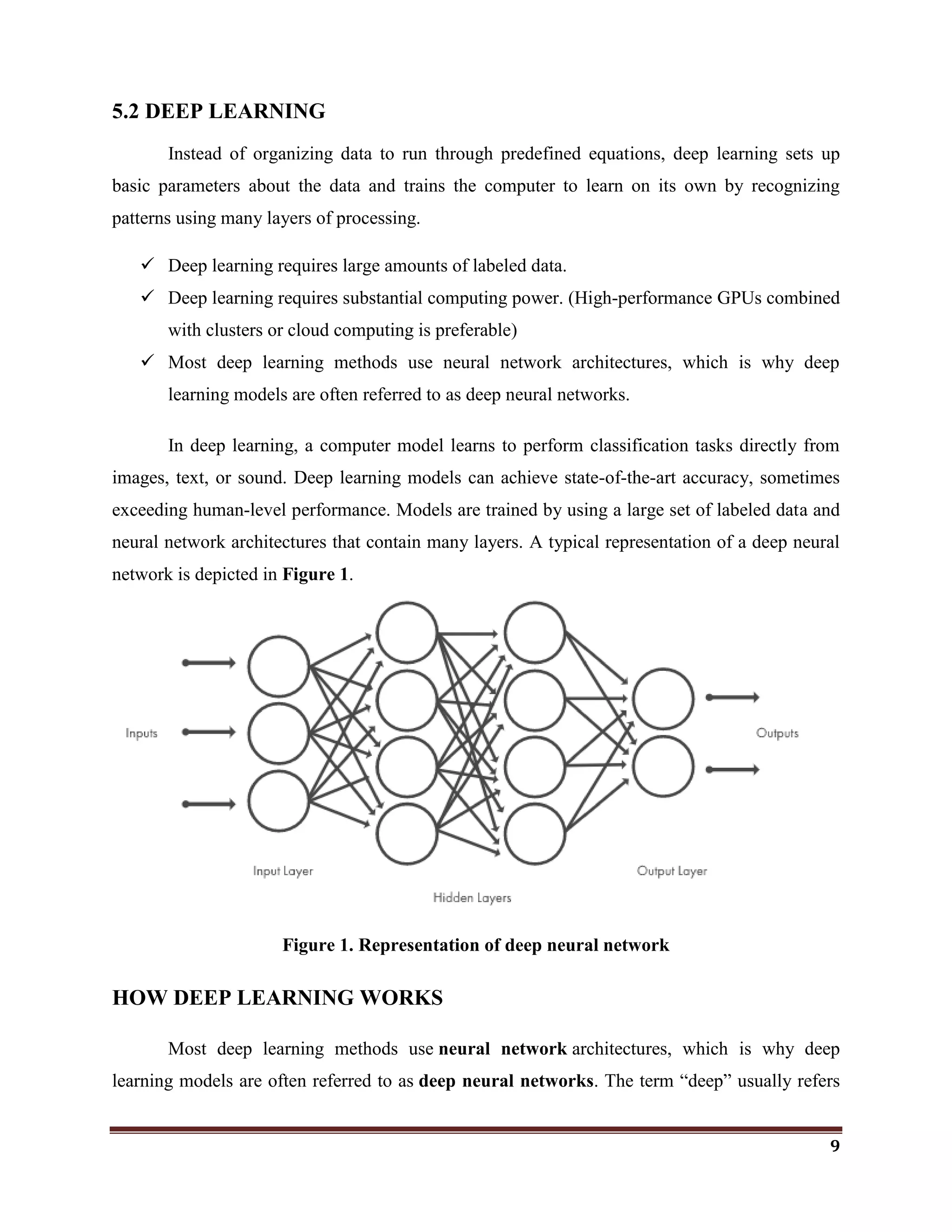
The document discusses classification as a key topic in machine learning, focusing on methods for classifying text and image data, specifically for detecting phishing websites and labeling CIFAR-10 images. It outlines the hardware and software specifications required for implementing machine and deep learning models, as well as reviews related literature and the functionalities of various R packages for machine learning and deep learning. The document emphasizes the importance of classification in big data analysis across multiple fields, including cybersecurity.

![22
Dataset uploads are resumable. If your Internet connection cuts out during an
upload, you'll be able to resume it later if you choose to.
If your upload has stopped before it completing, resume it using the
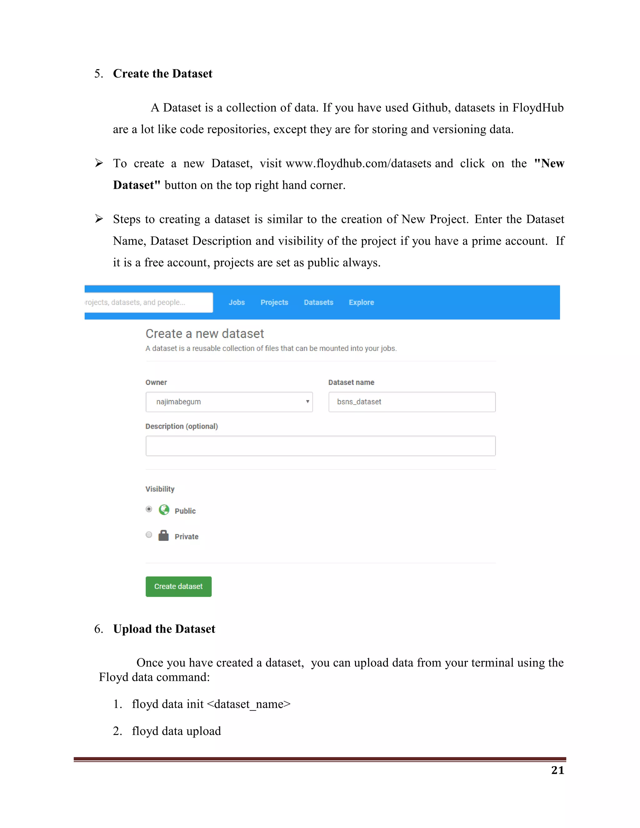
--resume or -r flag:
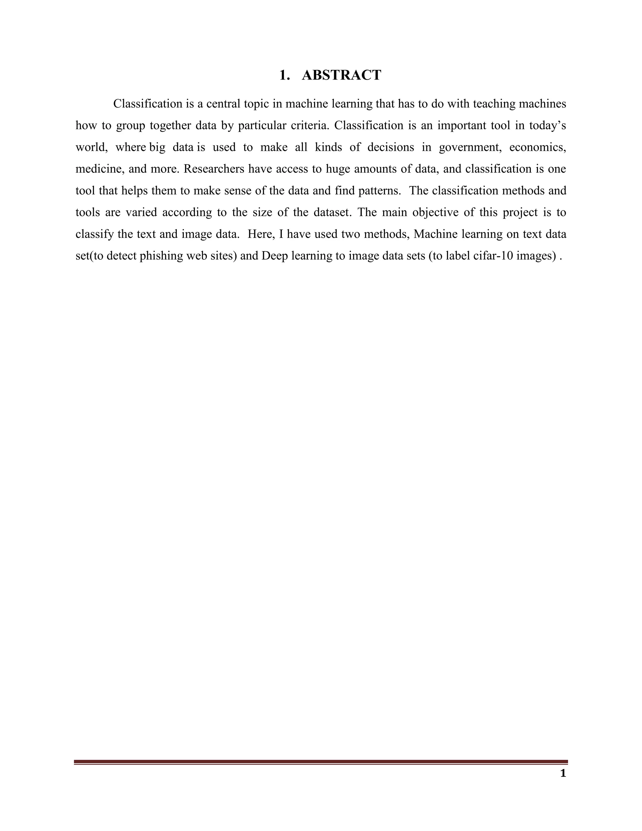
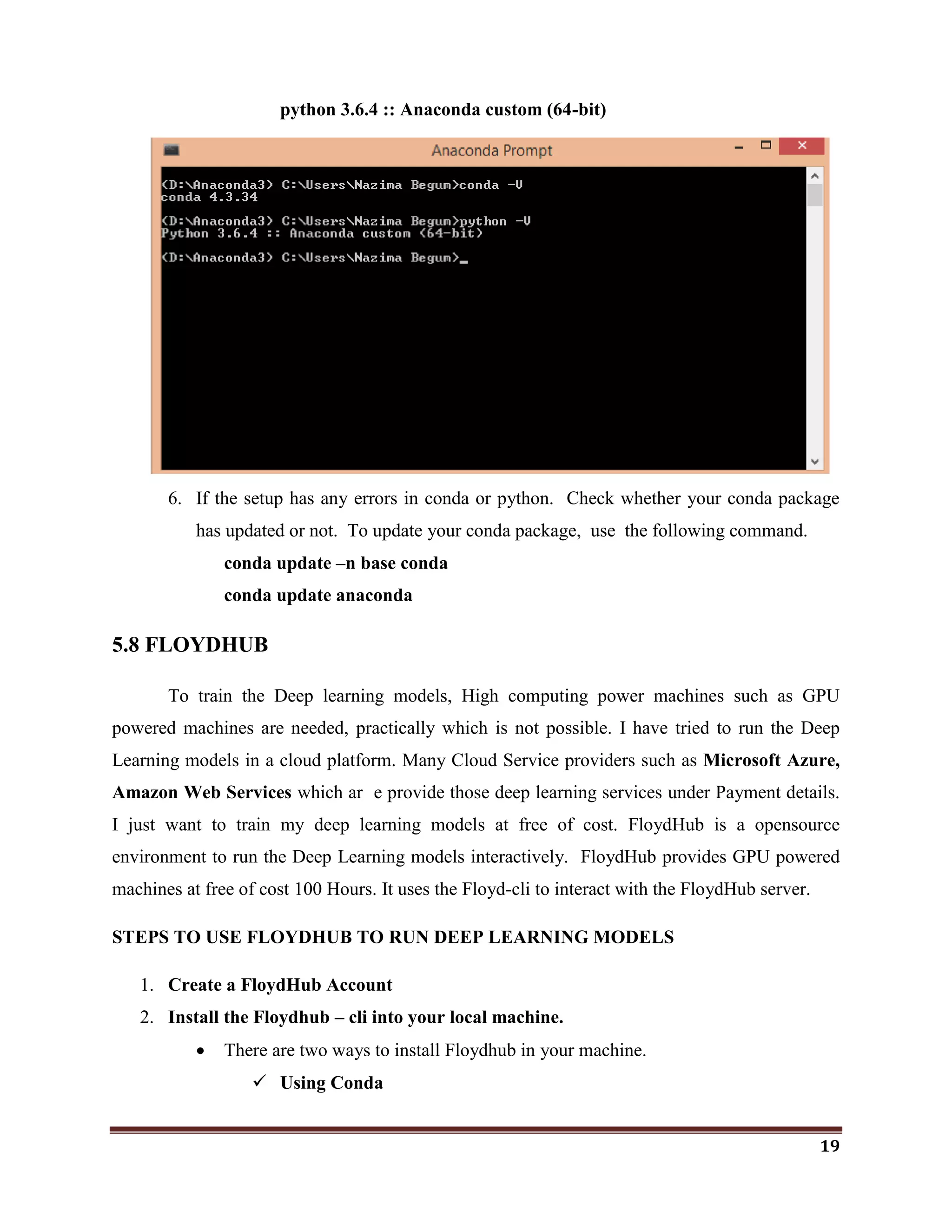
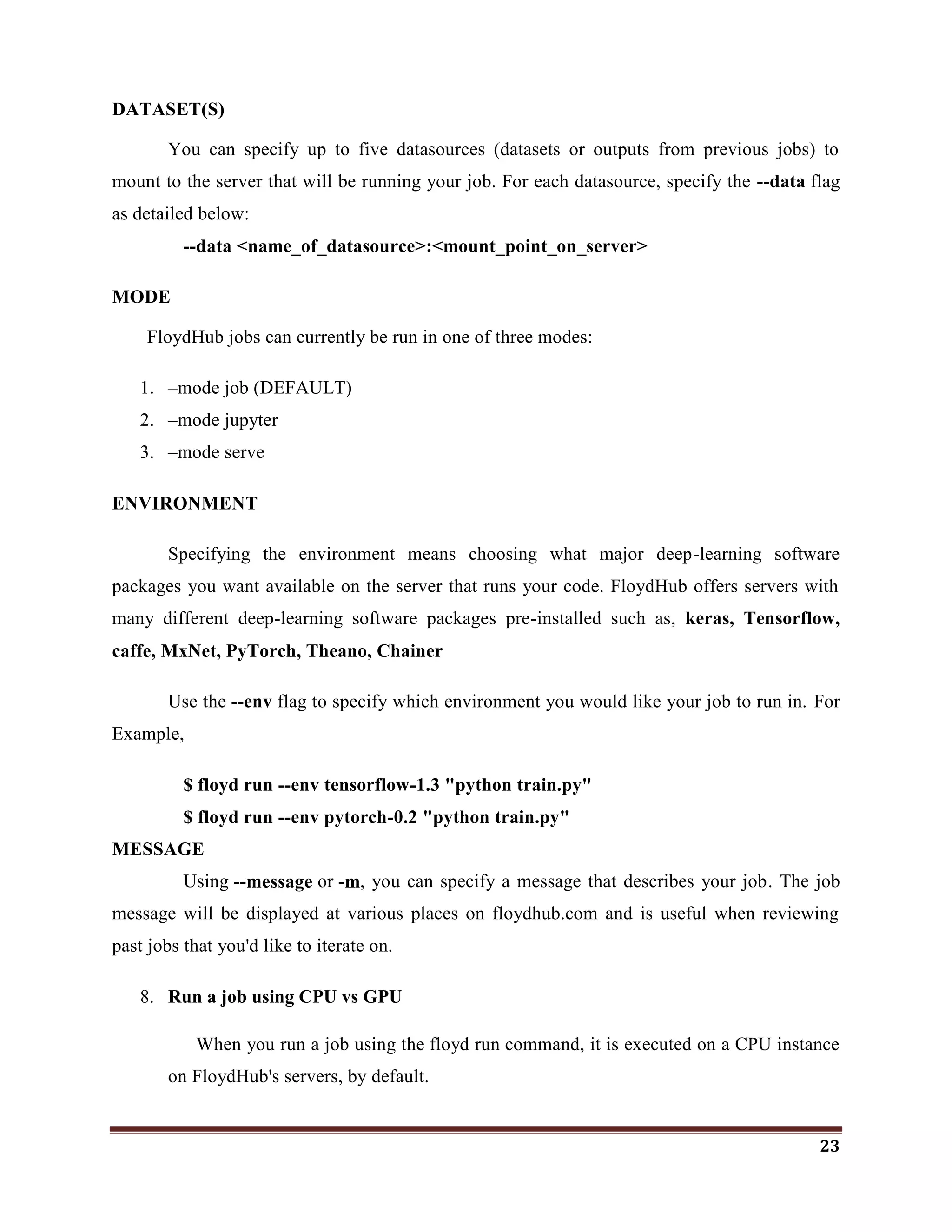
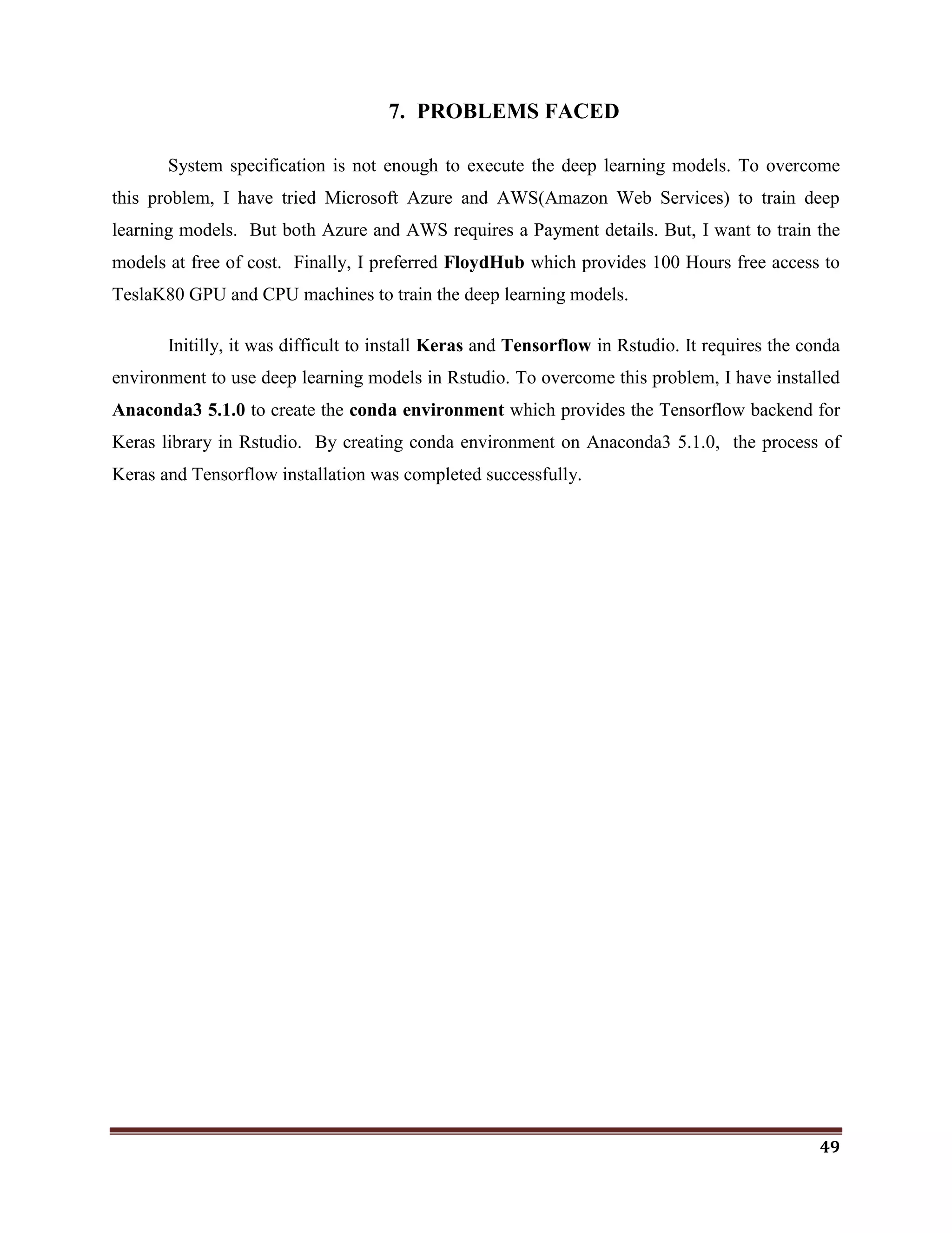
7. Run a job
Running jobs is the core action in the FloydHub workflow. A job pulls together
your code and dataset(s), sends them to a deep-learning server configured with the right
environment, and actually kicks off the necessary code to get the data science done.
The floyd run command is used to run the job.
PARTS OF THE floyd run COMMAND
[OPTIONS]
Instance Type : --cpu or --gpu or --cpu2 or --gpu2
Dataset(s) : --data
Mode : --mode
Environment : --env
Message : --message or -m
Tensorboard : --tensorboard
INSTANCE TYPE
To specify the instance type means to choose what kind of FloydHub instance your job
will run on. Think of this as a hardware choice rather than a software one. (The software
environment is declared with the Environment (--env) OPTION of floyd run command.)
Floyd run Flag Instance type Description
--gpu GPU Tesla K80 GPU Machine
--gpu2 GPU Tesla V100 GPU Machine
--cpu CPU 2 core low performance CPU Machine
--cpu2 CPU 8 core high performance CPU Machine](https://image.slidesharecdn.com/classificationwithr-180501074205/75/Classification-with-R-22-2048.jpg)

![28
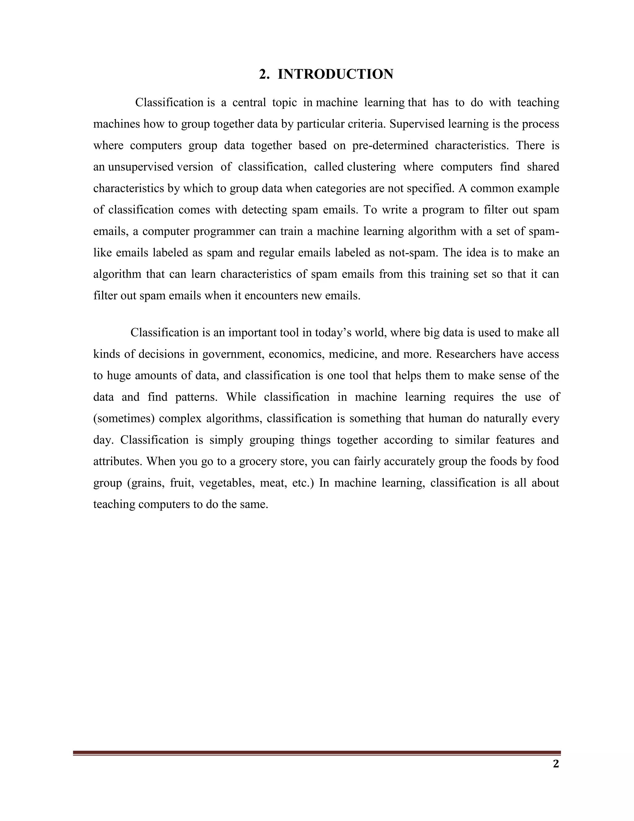
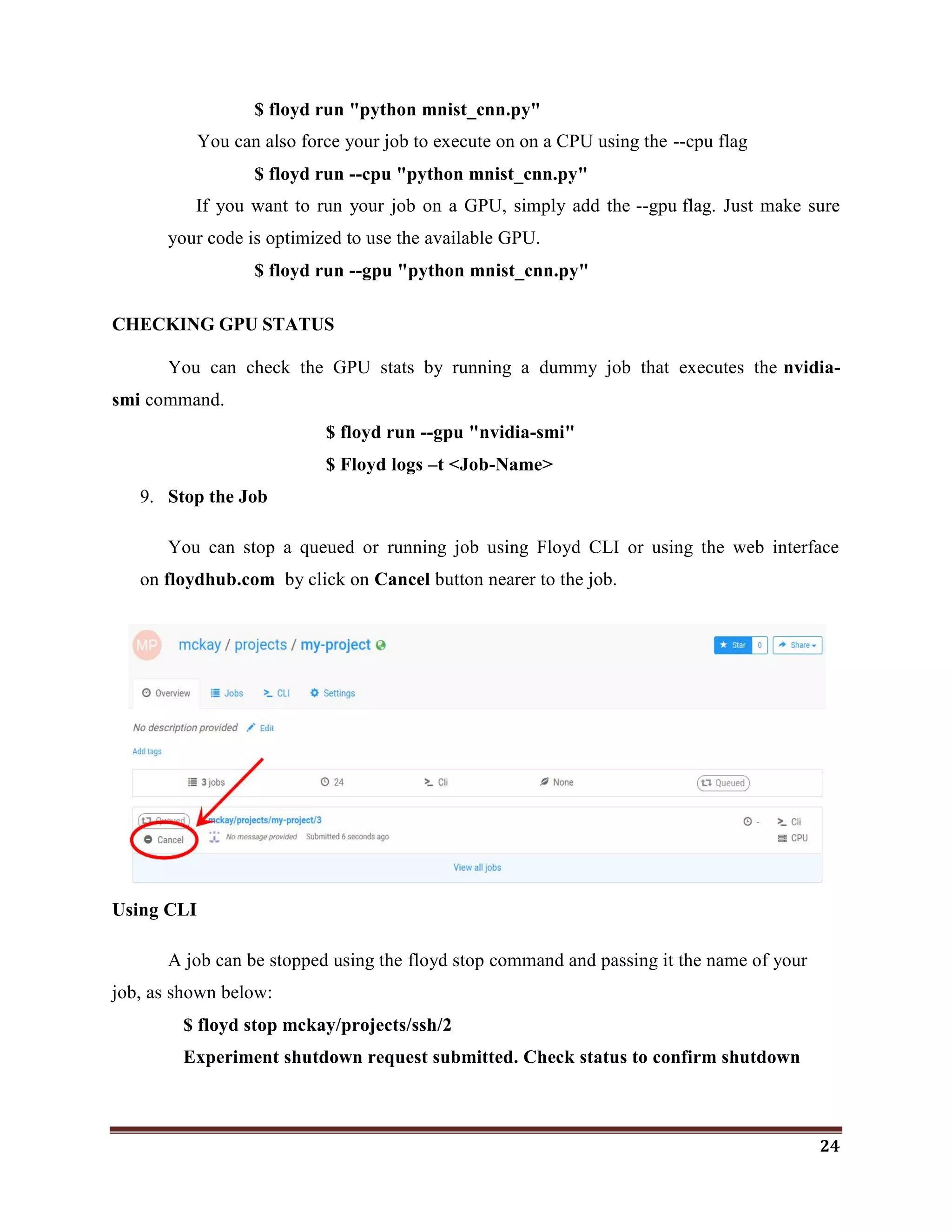
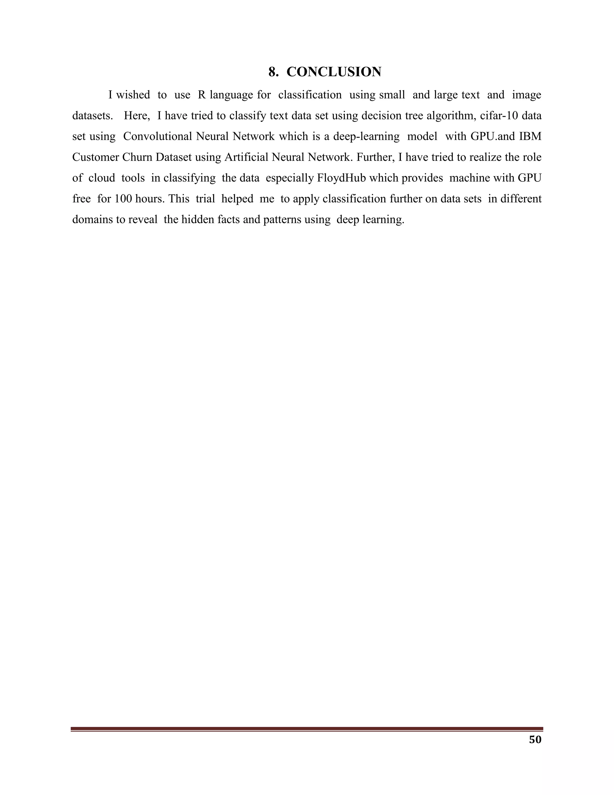
DATASET
I used a dataset of phishing website publicly available on the machine learning repository
provided by UCI. You don‘t have to download the dataset yourself as it is included directly in
this repository (dataset.csv le) and was downloaded on your machine when you cloned this
repository.
https://archive.ics.uci.edu/ml/datasets.html
https://www.phishtank.com/
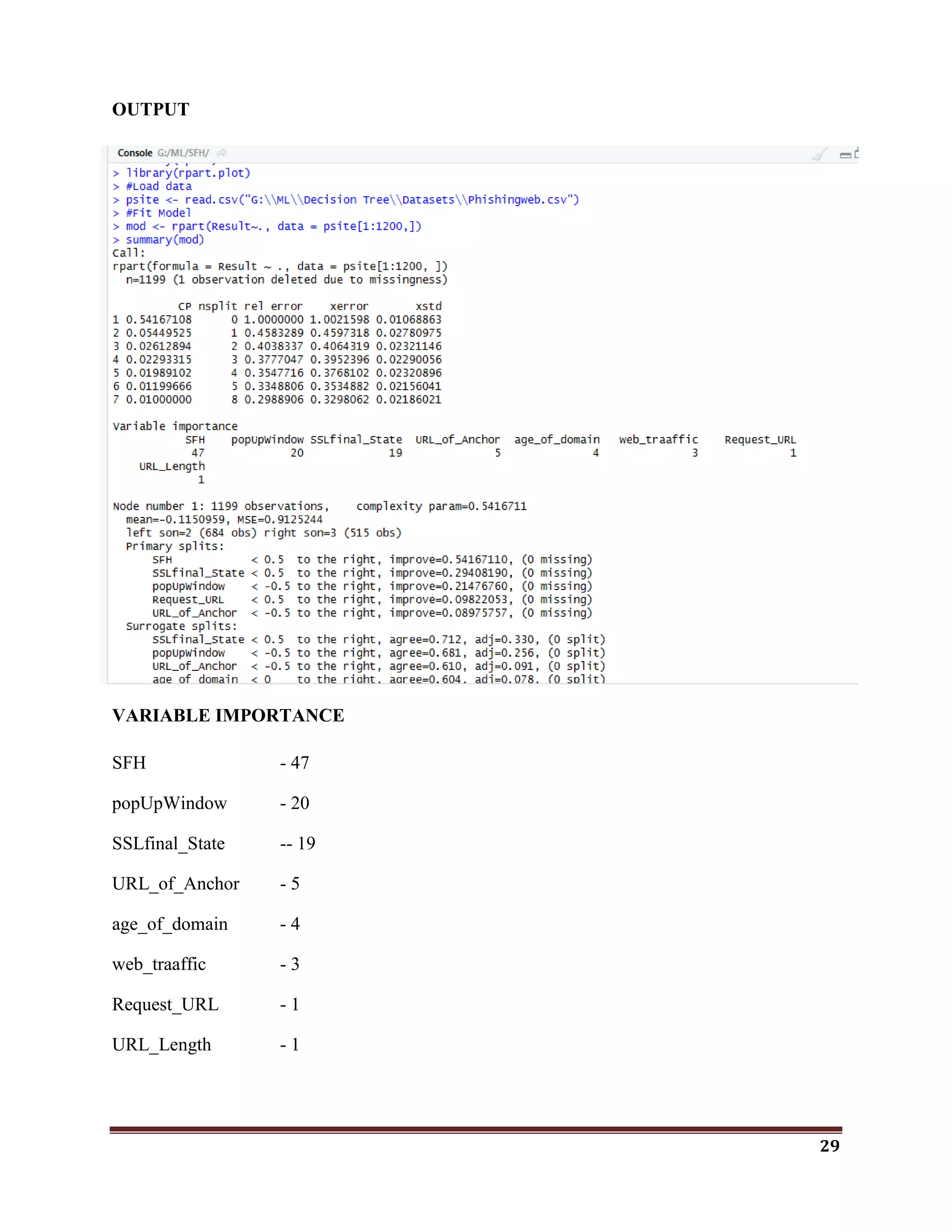
6.1.2 FIND THE MINIMAL EFFECTIVE ATTRIBUTES
CODE
#import package
library(rpart)
library(rpart.plot)
#Load data
psite <- read.csv("G:MLDecision TreeDatasetsPhishingweb.csv")
#Fit Model
mod <- rpart(Result~., data = psite[1:1200,])
summary(mod)
rpart.plot(mod, type= 4, extra= 101)
p <- predict(mod, psite[,1:9])
table(p,psite$Result)](https://image.slidesharecdn.com/classificationwithr-180501074205/75/Classification-with-R-28-2048.jpg)
![31
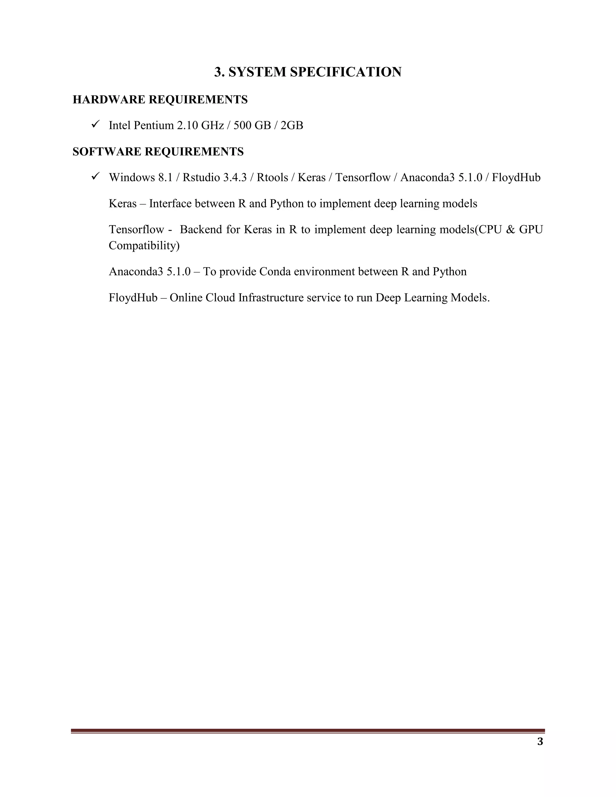
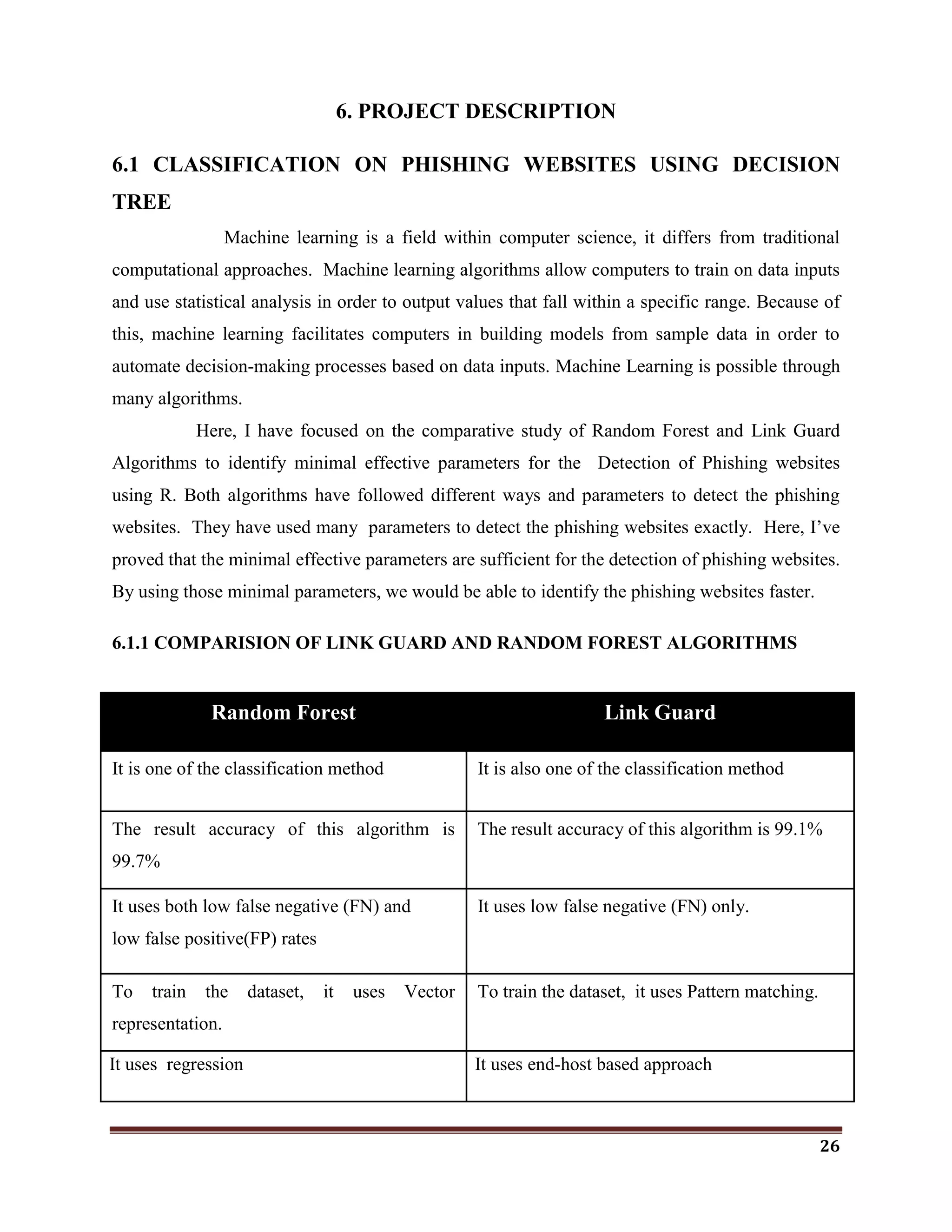
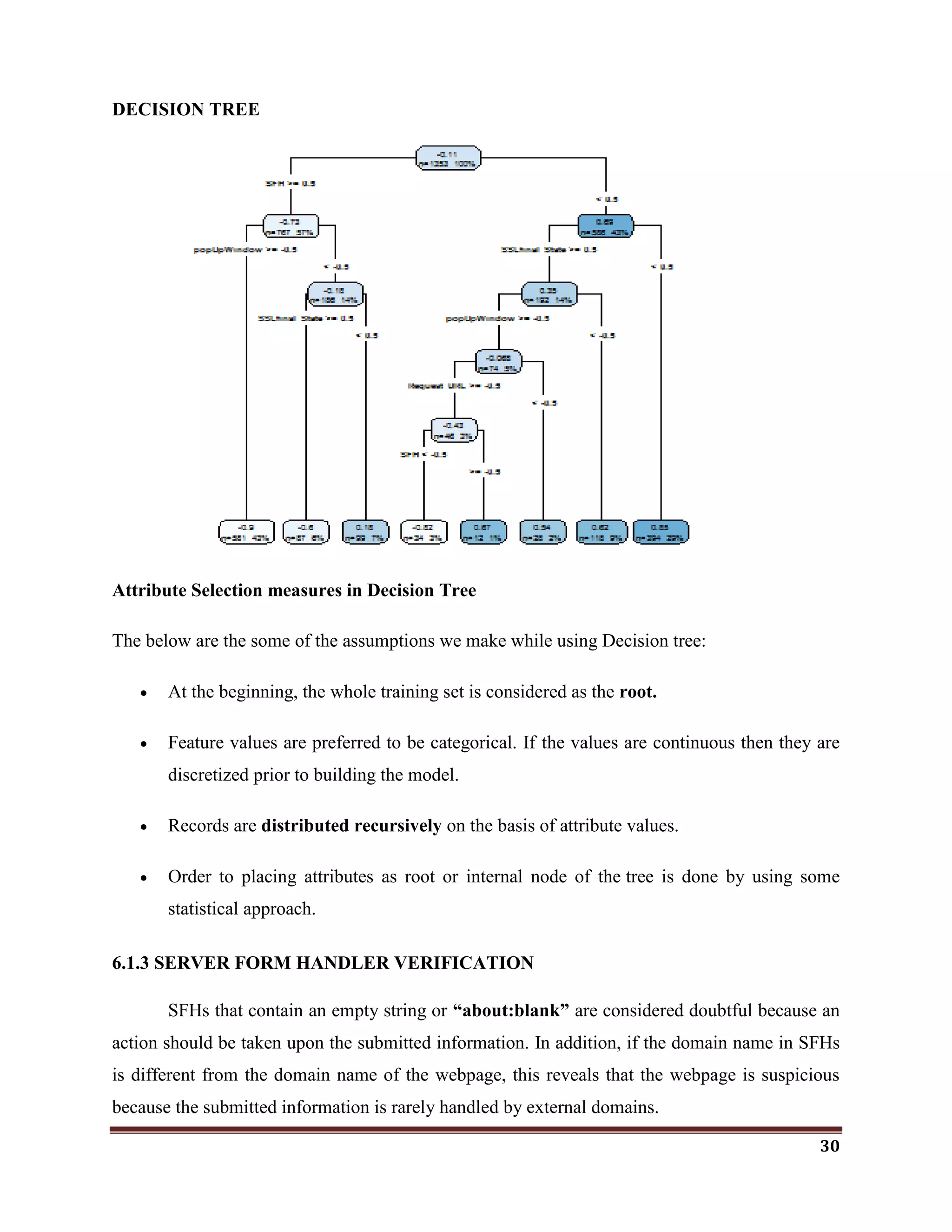
Rule:IF
SFH is "about: blank" Or Is Empty → Phishing
SFH Refers To A Different Domain → Suspicious
Otherwise → Legitimate
In the Decision tree, Server Form Handler(SFH) is set to be root. It indicates that SFH
plays a vital role in detecting phishing websites.
The importance of SFH variable is 47.
So, I tried to prove that, the SFH is a Minimal effective parameter to identify the
phishing websites.
For that, the SFH is extracted from the Link. If SFH occurs the FP(False Positive) value
is set to be 1. else set to be -1. If possibilities of SFH in the Link is founded FP value is
set to be 0.
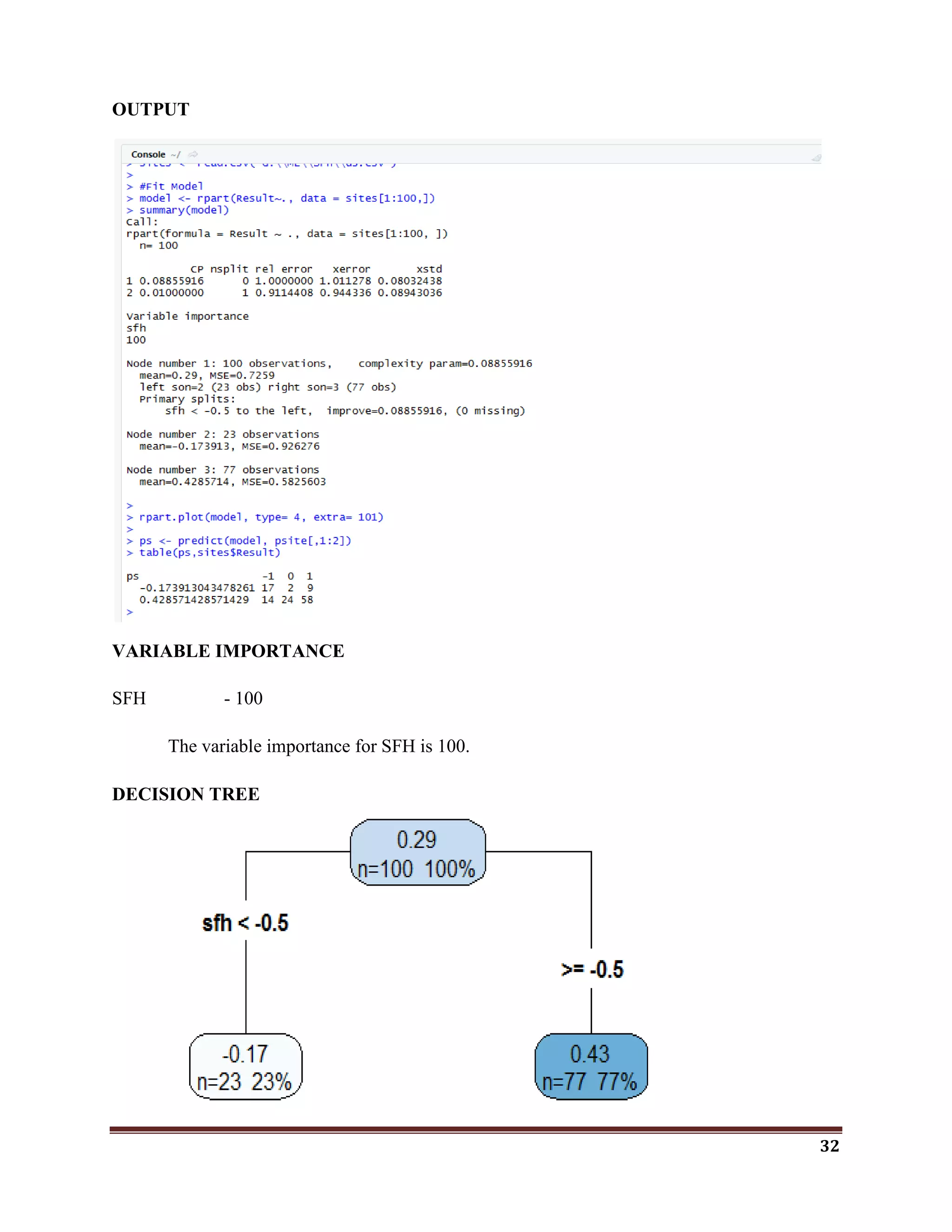
CODE TO CHECK WHETHER THE SFH IS SUFFICIENT TO DETECT PHISHING
WEBSITES OR NOT
library(party)
library(rpart.plot)
#Load data
sites <- read.csv("G:MLSFHds.csv")
#Fit Model
model <- rpart(Result~., data = sites[1:100,])
summary(model)
rpart.plot(model, type= 4, extra= 101)
ps <- predict(model, psite[,1:2])
table(ps,sites$Result)](https://image.slidesharecdn.com/classificationwithr-180501074205/75/Classification-with-R-31-2048.jpg)
![34
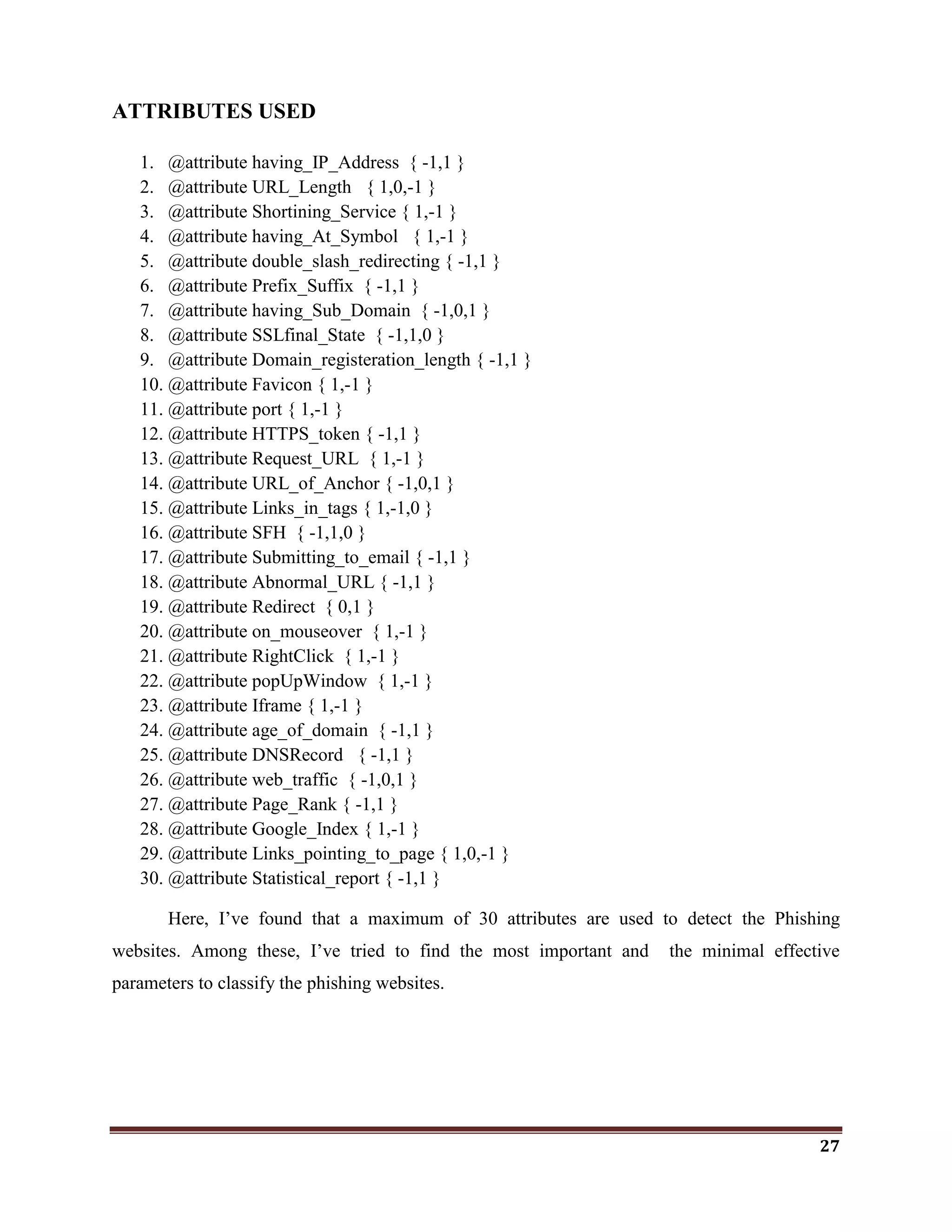
sites <- read.csv("G:MLSFHpone.csv")
#Fit Model
model <- rpart(result~., data = sites[1:100,])
summary(model)
rpart.plot(model, type= 4, extra= 101)
ps <- predict(model, sites[,1:2])
table(ps,sites$result)
OUTPUT
VARIABLE IMPORTANCE
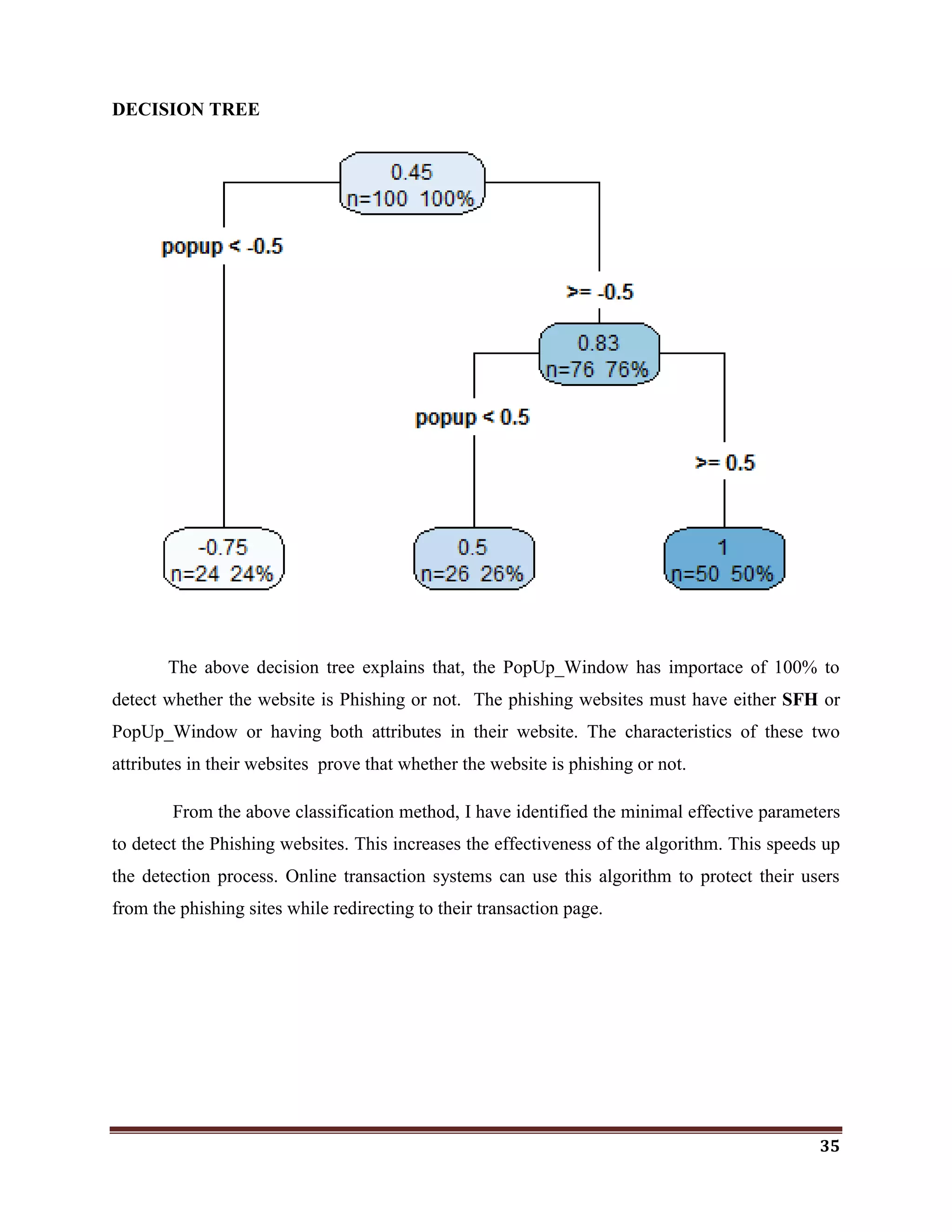
Popup - 100](https://image.slidesharecdn.com/classificationwithr-180501074205/75/Classification-with-R-34-2048.jpg)
![37
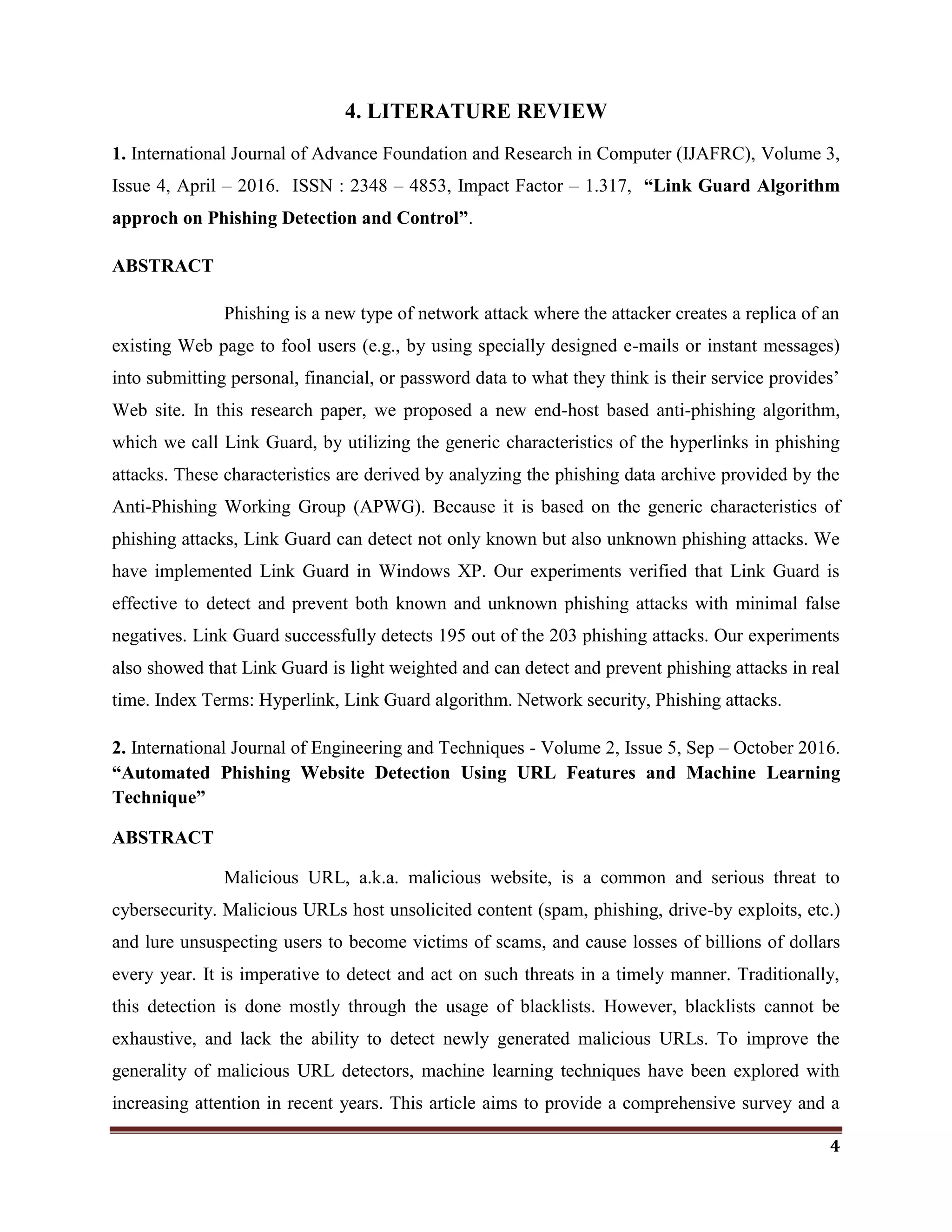
INPUT [32x32x3] will hold the raw pixel values of the image, in this case an image of width
32, height 32, and with three color channels R,G,B.
CONV layer will compute the output of neurons that are connected to local regions in the
input, each computing a dot product between their weights and a small region they are
connected to in the input volume. This may result in volume such as [32x32x12] if we
decided to use 12 filters.
RELU layer will apply an elementwise activation function, such as
the max(0,x)max(0,x) thresholding at zero. This leaves the size of the volume unchanged
([32x32x12]).
POOL layer will perform a downsampling operation along the spatial dimensions (width,
height), resulting in volume such as [16x16x12].
ConvNets transform the original image layer by layer from the original pixel values to the
final class scores. Note that some layers contain parameters and other don‘t. In particular, the
CONV/FC layers perform transformations that are a function of not only the activations in the
input volume, but also of the parameters (the weights and biases of the neurons). On the other
hand, the RELU/POOL layers will implement a fixed function. The parameters in the CONV/FC
layers will be trained with gradient descent so that the class scores that the ConvNet computes
are consistent with the labels in the training set for each image.
6.2.2 CIFAR-10 DATASET
The CIFAR-10 dataset consists of 60000 32x32 colour images in 10 classes, with 6000
images per class.
There are 50000 training images and 10000 test images. The dataset is divided into five
training batches and one test batch, each with 10000 images. The test batch contains exactly
1000 randomly-selected images from each class. The training batches contain the remaining
images in random order, but some training batches may contain more images from one class than
another.
The Classes are airplane, automobile, bird, cat, deer, dog, frog, horse, ship, and truck.
The Cifar-10 dataset is collected from https://www.cs.toronto.edu/~kriz/cifar.html](https://image.slidesharecdn.com/classificationwithr-180501074205/75/Classification-with-R-37-2048.jpg)
![42
The softmax function is a more generalized logistic activation function which is used for
multiclass classification.
2.ReLU(Rectified Linear Unit) Activation Function
The ReLU is half rectified (from bottom).It is f(s) is zero when z is less than zero and f(z)
is equal to z when z is above or equal to zero.
Range: [ 0 to infinity)
The function and its derivative both are monotonic.
But the issue is that all the negative values become zero immediately which decreases the
ability of the model to fit or train from the data properly. That means any negative input given to
the ReLU activation function turns the value into zero immediately in the graph, which in turns
affects the resulting graph by not mapping the negative values appropriately.
Here, I have used ReLU and Softmax Activation functions in CNN Architechture.
softmax gives the probability of output classes.
If the resulting vector for a classification program is [0 .1 .1 .75 0 0 0 0 0 .05], then this
represents a 10% probability that the image is a 1, a 10% probability that the image is a 2, a 75%
probability that the image is a 3, and a 5% probability that the image is a 9](https://image.slidesharecdn.com/classificationwithr-180501074205/75/Classification-with-R-42-2048.jpg)


![TEAM.MAJOR[1] project based on the .pptx](https://cdn.slidesharecdn.com/ss_thumbnails/team-240624193657-6c8dbe6e-thumbnail.jpg?width=640&height=640&fit=bounds)


![[DSC Europe 25] Dunja Adzic Jovanovic - AI and Cybersecurity: Defending Data ...](https://cdn.slidesharecdn.com/ss_thumbnails/o1zylpbhrtwnixxq2xj8-7-251211083048-185086f6-thumbnail.jpg?width=640&height=640&fit=bounds)
![[DSC Europe 25] Tatevik Maytesyan - How to actually use AI in marketing: gett...](https://cdn.slidesharecdn.com/ss_thumbnails/tjo626lsqdgfntbgl2mw-4-251216103155-e36cd239-thumbnail.jpg?width=640&height=640&fit=bounds)

![[DSC Europe 25] Ivan Peric - Intelligence Swarm Logic and Techno-Functional M...](https://cdn.slidesharecdn.com/ss_thumbnails/7my7c97fsduiccadgavw-2-251212103249-5a03f7c6-thumbnail.jpg?width=640&height=640&fit=bounds)

![[DSC Europe 25] Branko Urosevic -Rethinking Financial Talent: Integrating Cod...](https://cdn.slidesharecdn.com/ss_thumbnails/8jjrus8ttko6qj64f58f-3-251212103250-642c6374-thumbnail.jpg?width=640&height=640&fit=bounds)

![[DSC Europe 25] Hans Kleinsman - The Compliance Gearbox: How Tax Tech Mediate...](https://cdn.slidesharecdn.com/ss_thumbnails/dxdytie1toel0hr90bjs-2-251212103250-174fdbe7-thumbnail.jpg?width=640&height=640&fit=bounds)


![[DSC Europe 25] Dusan Nesic - Securing Tomorrow’s Infrastructure: Why Cyber-P...](https://cdn.slidesharecdn.com/ss_thumbnails/qikbszfftyowjm2q6duw-1-251211083848-8f2ead6b-thumbnail.jpg?width=640&height=640&fit=bounds)
![[DSC Europe 25] Miodrag Pesovic & Vladislav Radonjic - Federated Data Archite...](https://cdn.slidesharecdn.com/ss_thumbnails/gsbe3y5it5uhndi4e08e-1-251212103249-f1008e0c-thumbnail.jpg?width=640&height=640&fit=bounds)


![[DSC Europe 25] Uros Pesic - The Reality of AI in Marketing.pdf](https://cdn.slidesharecdn.com/ss_thumbnails/rtkodnmtycovsllvzsyn-9-251215095918-b0c6bfe3-thumbnail.jpg?width=640&height=640&fit=bounds)


![[DSC Europe 25] Katherine Forrest - AI NOW: Understanding the Velocity of Cha...](https://cdn.slidesharecdn.com/ss_thumbnails/wvvbruqfrci0sfq9xwgb-4-251212104007-e5ad1987-thumbnail.jpg?width=640&height=640&fit=bounds)
