project

1. 1
CLASSIFICATION OF THYROID DISEASE : SVM APPROACH
Anjali Sinha(A0178476L), Viknesh Kumar Balakrishnan(A0178304A),
Sabrish Gopalakrishnan(A0178314E)
Institute of Information Sciences, National University Of Singapore
ABSTRACT
Analyzing medical data set involves challenging tasks because of
the minute variations for analysis. Medical database consists of
different modalities taken under varied conditions with variable
accuracy of annotation. Classification is one of the fundamental
tasks involved in any process. The input for a classification is a
set of training records where each record has several attributes.
The main objective of this report is to apply SVM for multiclass
classification and compare the different models obtained by fine
tuning it, for thyroid data set from UCI. This is important to ensure
a stable knowledge base can be established in the hybrid model
for solving complex learning tasks, such as in medical diagnosis
and prognosis applications.
1. INTRODUCTION
Thyroid gland is an endocrine gland found in the lower part of
human neck, which helps in secretion of thyroid hormones, and
maintaining and balancing the body’s metabolism. Generally two
types of hormones are produced by thyroid glands, namely
levothyroxine (T3) and triiodothyroxine (T4). The functionalities
of these two hormones are that it helps in production of well-
balanced amount of proteins, regulating the body’s temperature,
and maintaining overall production of energy.
Thyroid disease can be divided normally into two types, these are
hypothyroidism and hyperthyroidism. Hypothyroidism - it is the
state of insufficient or too little production of hormones.
Hyperthyroidism - when glands produces excessive amount of
thyroid hormones. The issues related to thyroid disease should
never be underestimated by thyroid patient because it may cause
disease like thyroid storm (type of critical hyperthyroidism) and
myxedema (the last stage of untreated hypothyroidism) which
may result in death.
Recent studies have shown that women are 5 to 8 times more
prone to thyroid disease in comparison from men.
Hypothyroidism can even be associated with pregnancy in women
as well. For correct diagnosis of thyroid disease, interpretation of
thyroid data must be carefully observed beside the clinical
examination because even a minute fluctuation in data can cause
severe problems.
The study aims to diagnose thyroid disease’s using several
classifiers mechanism. Also based upon this diagnosis it will open
the way for various ill disorder diagnosis for future clinically
examine data and increase the chance of progress.
The thyroid dataset used for this analysis has been taken from
UCI repository and has 21 attributes and 7200 records originally.
The attributes present in the dataset are :
Attributes Description
age continuous
sex ‘M’,’F’,’NA’
on thyroxine f, t
query on thyroxine f, t
On antithyroid medication f, t
sick f, t
pregnant f, t
Thyroid surgery f, t
I131 treatment f, t
query hypothyroid f, t
query hyperthyroid f, t
lithium f, t
goitre f, t
tumor f, t
hypopituitary f, t
psych f, t
TSH continuous
T3 continuous
TT4 continuous
T4U continuous
FTI continuous
The target classes for this dataset are :
1: decreased binding protein, 2: increased binding protein, 3:
negative
We deal with categorical data by transformation/one hot
encoding and then standardize the continuous data. As the
number of classes is skewed, we do data balancing using the R
package SMOTE, which helps us get similar number of
instances for each class. Data imputation was done using MICE
package. We leverage scikit-learn python package for our
analysis. A train-test split of 80:20 is used here.
2. BASELINE APPROACH
The baseline approach involves classification of thyroid disease
using the basic SVM with default parameters. This serves as a
basis for comparison of results.

2. 2
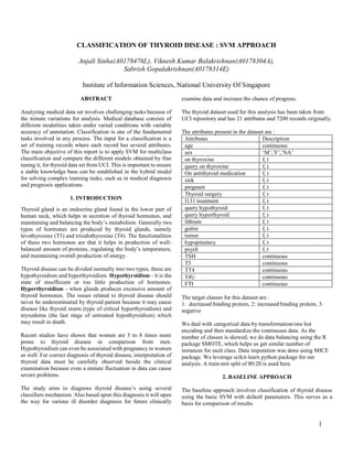
2.1. Simple SVM Classifier using Linear Kernel
Here we set the kernel of the SVM classifier to “linear”. We
observe the following:
Accuracy : 0.920364050057
Precision : 0.920 (+/-0.028)
Recall : 0.930 (+/-0.027)
Confusion Matrix :
A P Class 1 Class 2 Class 3
Class 1 187 0 4
Class 2 0 308 11
Class 3 18 37 314
2.2. Simple SVM Classifier using RBF Kernel
Here we set the kernel of the SVM classifier to “rbf”. We observe
the following:
Accuracy : 0.763367463026
Precision : 0.804 (+/-0.028)
Recall : 0.722 (+/-0.041)
Confusion Matrix :
A P Class 1 Class 2 Class 3
Class 1 117 0 74
Class 2 0 227 92
Class 3 17 25 327
2.4. Simple SVM Classifier using Sigmoid Kernel
Here we set the kernel of the SVM classifier to “sigmoid”. We
observe the following:
Accuracy : 0.668941979522
Precision : 0.770 (+/-0.073)
Recall : 0.617 (+/-0.039)
Confusion Matrix :
A P Class 1 Class 2 Class 3
Class 1 61 0 130
Class 2 0 208 111
Class 3 19 31 319
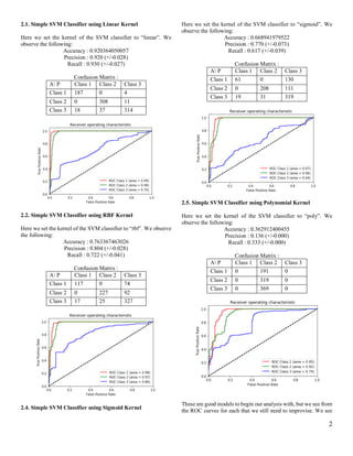
2.5. Simple SVM Classifier using Polynomial Kernel
Here we set the kernel of the SVM classifier to “poly”. We
observe the following:
Accuracy : 0.362912400455
Precision : 0.136 (+/-0.000)
Recall : 0.333 (+/-0.000)
Confusion Matrix :
A P Class 1 Class 2 Class 3
Class 1 0 191 0
Class 2 0 319 0
Class 3 0 369 0
These are good models to begin our analysis with, but we see from
the ROC curves for each that we still need to improvise. We see

3. 3
that linear kernel performs the best amongst all(though we still
need to improvise). Also we observe that polynomial kernel
performs very badly, which means that the baseline model it is not
well suited for the dataset and we didn’t taken this up for further
optimization.
3. PROPOSED APPROACH
The baseline approach, doesn’t quite perform very well, as we can
see from the evaluation metrics computed for each of the baseline
approaches. We will now try to improvise the model, by feature
engineering techniques and fine tune the model hyper parameters,
to compare the performances.
3.1. Feature Engineering using RFECV
Recursive Feature Elimination with Cross Validation (RFECV),
is used to rank features to select the best out of them, which are
critical in determining the model’s performance. Using RFECV,
we boil down to 18 features, from the 21 features we had
originally.
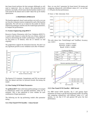
The graph below supports the elimination decision. We don’t see
any significant growth in cross validation score after 18 features :
The features I131.treatment, hypopituitary and T4U are removed
from the dataset and then we proceed towards fine-tuning the
model.
3.2. Fine-Tuning SVM Model Parameters
The gridsearchCV from scikit-learn python package is leveraged
to exhaustively search over specified parameter values for an
estimator. This is also optimized to cross validate for each
combination of hyper parameters.
The following are the top performing models after parameter
tuning :
3.2.1. Fine-Tuned SVM Classifier – Linear Kernel
Here, we vary the C parameter for linear kernel. On tuning and
comparing exhaustively with different values of C, we see that
C=250 gives the best performance.
This plot shows how Train(Orange) and Test(Blue) Accuracy
vary with C.
Accuracy : 0.943117178612
Precision : 0.940 (+/-0.009)
Recall : 0.949 (+/-0.009)
Confusion Matrix :
A P Class 1 Class 2 Class 3
Class 1 191 0 0
Class 2 0 311 8
Class 3 7 35 327
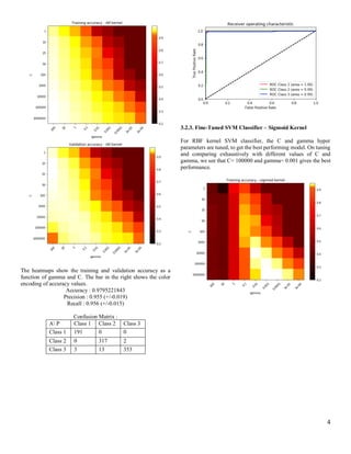
3.2.2. Fine-Tuned SVM Classifier – RBF Kernel
For RBF kernel SVM classifier, the C and gamma hyper
parameters are tuned, to get the best performing model. On tuning
and comparing exhaustively with different values of C and
gamma, we see that C=25 and gamma=100 gives the best
performance.

4. 4
The heatmaps show the training and validation accuracy as a
function of gamma and C. The bar in the right shows the color
encoding of accuracy values.
Accuracy : 0.9795221843
Precision : 0.955 (+/-0.019)
Recall : 0.956 (+/-0.015)
Confusion Matrix :
A P Class 1 Class 2 Class 3
Class 1 191 0 0
Class 2 0 317 2
Class 3 3 13 353
3.2.3. Fine-Tuned SVM Classifier – Sigmoid Kernel
For RBF kernel SVM classifier, the C and gamma hyper
parameters are tuned, to get the best performing model. On tuning
and comparing exhaustively with different values of C and
gamma, we see that C= 100000 and gamma= 0.001 gives the best
performance.

5. 5
The heatmaps show the training and validation accuracy as a
function of gamma and C. The bar in the right shows the color
encoding of accuracy values.
Accuracy : 0.941979522184
Precision : 0.937 (+/-0.013)
Recall : 0.948 (+/-0.014)
Confusion Matrix :
A P Class 1 Class 2 Class 3
Class 1 191 0 0
Class 2 0 311 8
Class 3 8 35 326
4. EXPERIMENTAL RESULTS
4.1. Results
Model Accuracy Precision Recall
1 Simple SVM Classifier
using Linear Kernel
0.9203 0.920 0.930
2 Simple SVM Classifier
using RBF Kernel
0.7633 0.804 0.722
3 Simple SVM Classifier
using Sigmoid Kernel
0.6689 0.770 0.617
4 Simple SVM Classifier
using Polynomial Kernel
0.3629 0.136 0.333
5 Fine-tuned SVM
Classifier using Linear
Kernel
0.9431 0.940 0.949
6 Fine-tuned SVM
Classifier using RBF
Kernel
0.9795 0.955 0.956
7 Fine-tuned SVM
Classifier using sigmoid
Kernel
0.9419 0.937 0.948
We see that the best model that should be used for Thyroid dataset
is the Fine-tuned SVM classifier using RBF kernel, with
hyperparameters C=25 and gamma=100.
5. CONCLUSIONS
The optimal model that should be used for this dataset is the Fine-
tuned SVM classifier using RBF kernel, with C=25 and
gamma=100.
We observe that for the simple SVM classifier, the linear kernel
worked the best amongst the 4 kernels, but after fine-tuning we
see that the RBF kernel is the winner. The validation accuracy is
seen to rise from 0.9203 to 0.9795 after fine tuning the hyper
parameters.
The feature elimination technique helped us reduce the data in
hand and get rid of the features that were not so significant in
contributing much towards the target prediction, without affecting
any of the scores much.
6. REFERENCES
[1] HalifeKodaz, Seral ,AhmetArslan , SalihGune: Medical application
of information gain based artificial immune recognition system (AIRS):
Diagnosis of thyroid disease.
[2] UCI Machine Learning Repository: Thyroid Disease DataSet
https://archive.ics.uci.edu/ml/datasets/Thyroid+Disease
[3] FeyzullahTemurtas: A comparative study on thyroid disease
diagnosis using neural networks.
[4] M.P.Gopinath, Comparative Study on Classification Algorithm for
Thyroid Data Set.
[5] For analysis and comparision : http://scikit-
learn.org/stable/modules/svm.html