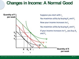
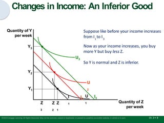
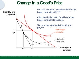
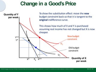
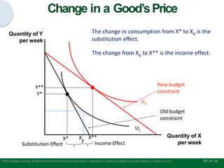
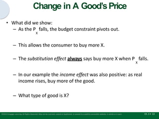
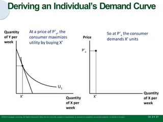
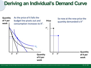
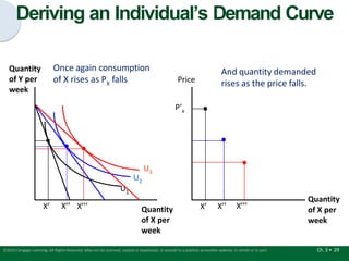
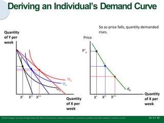
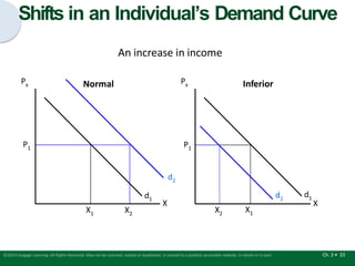
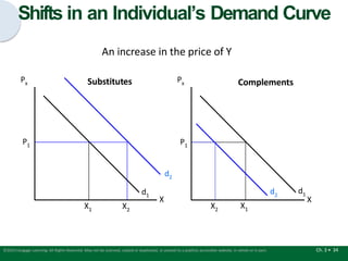
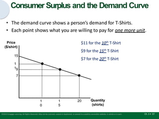
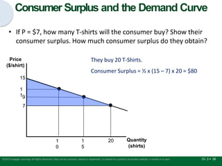
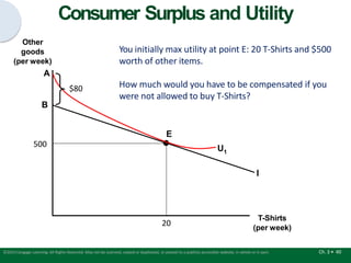
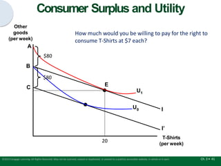
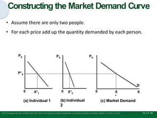
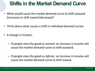
Walter Nicholson
1
Amherst College
Christopher Snyder
Dartmouth College
PowerPoint Slide Presentation | Philip Heap, James Madison University
©2015 Cengage Learning. All Rights Reserved. May not be scanned, copied or duplicated, or posted to a publicly accessible website, in whole or in part.
Demand
Curves
2
CHAPTER
3
Chapter Preview
Ch. 3 • 3
©2015 Cengage Learning. All Rights Reserved. May not be scanned, copied or duplicated, or posted to a publicly accessible website, in whole or in part.
• Last chapter you learned how an individual maximizes her utility.
– What were the two utility maximizing conditions?
• Now we will use the utility maximization model to show how to
derive an individual’s demand curve.
• From there, we can see how we get the market demand curve.
Individual Demand Functions
Ch. 3 • 4
©2015 Cengage Learning. All Rights Reserved. May not be scanned, copied or duplicated, or posted to a publicly accessible website, in whole or in part.
• A demand function: representation of how quantity demanded
depends on prices, income, and preferences.
• Quantity of X demanded = d (P , P , I; preferences)
X X Y
• The amount of soda you demand depends on: price of soda, price
of a related goods, your income, and your preferences.
• We will assume that over the relevant time frame, preferences
remain the same.
Individual Demand Functions
Ch. 3 • 5
©2015 Cengage Learning. All Rights Reserved. May not be scanned, copied or duplicated, or posted to a publicly accessible website, in whole or in part.
• Suppose that both the prices of the goods you buy and your
income double. How do you change your behavior?
• You don’t. What matters is the relative price of goods and the
real value of your income.
• Demand functions are homogeneous. Quantity demanded does
not change when prices and income change proportionally.
– P X + P Y = I vs. 2P X + 2P Y = 2I
X Y X Y
Changes in Income
Ch. 3 • 6
©2015 Cengage Learning. All Rights Reserved. May not be scanned, copied or duplicated, or posted to a publicly accessible website, in whole or in part.
• What happens to the quantity purchased of some good as your
income increases?
• Depends on whether the good is normal or inferior.
– A normal good is a good that is bought in greater quantities as
income increases.
– An inferior good is a good that is bought in smaller quantities
as income increases.
Changes in Income: A Normal Good
Quantity of Y
per week
Quantity of X
per week
X
1
I
1
U
1
Suppose you start with I1
I2
Y2
Y1
X2
U
2
You maximize utility by buying X1 and Y1
Now your income increases to I2
You maximize utility by buying X2 and Y2
If your income increases to Y3, you buy X3
and Y3
U
3
X
3
Ch. 3 • 7
©2015 Cengage Learning. All Rights Reserved. May not be scanned, copied or duplicated, or posted to a publicly accessible website, in whole or in part.
Y3
I3
Changes in Income: An Inferior Good
Quantity of Y
per week
Quantity of Z
per week
Z Z
2 1
Y1
I
1
U
1
Suppose like before your income increases
from I to I
1 3
Now as your income increases, you buy
I2
Y2
U
2
Z
3
Y3
I3
more Y but buy less Z.
U3
So Y is normal and Z is inferior.
Ch. 3 • 8
©2015 Cengage Learning. All Rights Reserved. May not be scanned, copied or duplicated, or posted to a publicly accessible website, in whole or in part.
Change in A Good’sPrice
Ch. 3 • 9
©2015 Cengage Learning. All Rights Reserved. May not be scanned, copied or duplicated, or posted to a publicly accessible website, in whole or in part.
• What happens to the quantity purchased of some good when the
price of the good falls or rises?
• Substitution effect
– The effect on consumption due to a change in price holding
real income or utility constant.
• Income effect
– The effect on consumption due to a change in real income
caused by a change in price.
Change in a Good’sPrice
Quantity of Y
per week
Quantity of X
per week
constraint
U2
Old budget
constraint
U1
Y**
Y*
Ch. 3 • 10
©2015 Cengage Learning. All Rights Reserved. May not be scanned, copied or duplicated, or posted to a publicly accessible website, in whole or in part.
X**
X*
Initially a consumer maximizes utility on the
budget constraint at X*, Y*
A decrease in the price of X will cause the
budget constraint to pivot out.
The consumer now maximizes utility at
X**,Y**
New budget
Change in a Good’sPrice
Quantity of Y
per week
Quantity of X
per week
U1
New budget
constraint
U2
Old budget
constraint
Y**
Y*
Ch. 3 • 11
©2015 Cengage Learning. All Rights Reserved. May not be scanned, copied or duplicated, or posted to a publicly accessible website, in whole or in part.
X**
X* XB
To show the substitution effect: move the new
budget constraint back so that it is tangent to the
original indifference curve.
This shows how much of X and Y is purchased
assuming real income has not changed but X is now
cheaper.
Change in a Good’sPrice
Quantity of Y
per week
Quantity of X
per week
U1
New budget
constraint
U2
Old budget
constraint
Y**
Y*
XB
X*
Substitution Effect
The change in consumption from X* to XB is the
substitution effect.
The change from XB to X** is the income effect.
X**
Income Effect
Ch. 3 • 12
©2015 Cengage Learning. All Rights Reserved. May not be scanned, copied or duplicated, or posted to a publicly accessible website, in whole or in part.
Change in A Good’sPrice
Ch. 3 • 13
©2015 Cengage Learning. All Rights Reserved. May not be scanned, copied or duplicated, or posted to a publicly accessible website, in whole or in part.
• What did we show:
– As the P falls, the budget constraint pivots out.
X
– This allows the consumer to buy more X.
– The substitution effect always says buy more X when P falls.
X
– In our example the income effect was also positive: as real
income rises, buy more of the good.
– What type of good is X?
A Numerical Example
Ch. 3 • 14
©2015 Cengage Learning. All Rights Reserved. May not be scanned, copied or duplicated, or posted to a publicly accessible website, in whole or in part.
• Suppose you have $30. P = $3 and P
Burger Soda
= $1.50. You buy 5
burgers and 10 sodas in order to maximize utility.
• Now suppose P = $1.50
Burger
• If you still buy 5 burgers and 10 sodas you have $7.50 left over.
• At this point the MRS ≠ price ratio. Buy more burgers and less
soda: substitution effect
• With greater purchasing power can buy more burgers and more
soda: income effect
Substitution and Income Effects
Ch. 3 • 15
©2015 Cengage Learning. All Rights Reserved. May not be scanned, copied or duplicated, or posted to a publicly accessible website, in whole or in part.
• Any price change has both substitution and income effects. Why
is the substitution effect generally more important?
– In most cases income effects are small since the good
constitutes only a small portion of total spending.
• Think of perfect complements and perfect substitutes. What is
the size of the two effects?
Substitution and Income Effects
Right
Shoes
Left
Shoes
U1
I
Exxo
n
Mobi
l
I’
U1
I
Ch. 3 • 16
©2015 Cengage Learning. All Rights Reserved. May not be scanned, copied or duplicated, or posted to a publicly accessible website, in whole or in part.
I’
Substitution and Income Effects for Inferior
Goods
Ch. 3 • 17
©2015 Cengage Learning. All Rights Reserved. May not be scanned, copied or duplicated, or posted to a publicly accessible website, in whole or in part.
• What happens as the price of X increases?
– The substitution effects leads to more X.
– The income effect leads to less X.
– Since overall the consumption of X increases when the price of
X falls the substitution effect > income effect.
Substitution and Income Effects for Inferior
Goods
U1
Quantity of
X
per week
Quantity of
Y
per week
Y*
X*
The consumer starts by buying X* and Y*
If the price of X increases, the constraint pivots
in and the consumer now buy X** and Y**
U2
X**
Y**
Ch. 3 • 18
©2015 Cengage Learning. All Rights Reserved. May not be scanned, copied or duplicated, or posted to a publicly accessible website, in whole or in part.
Substitution and Income Effects for Inferior
Goods
U1
Quantity of
X
per week
Quantity of
Y
per week
Y*
X*
The substitution effect is from X* to XB
The income effect is from XB to X**
U2
X**
Y**
X
Ch. 3 • 19
©2015 Cengage Learning. All Rights Reserved. May not be scanned, copied or duplicated, or posted to a publicly accessible website, in whole or in part.
B
To show the substitution effect: move the new
budget constraint back so that it is tangent to the
original indifference curve.
Substitution and Income Effects for Inferior
Goods
Ch. 3 • 20
©2015 Cengage Learning. All Rights Reserved. May not be scanned, copied or duplicated, or posted to a publicly accessible website, in whole or in part.
• So for an inferior good:
– As the price rises (falls), the substitution effects says to buy
less (more)
– As the price rises (falls), the income effect says to buy more
(less) if the good is inferior.
– The substitution effect > income effect so as price rises (falls),
quantity falls (rises)
Giffen’sParadox
Ch. 3 • 21
©2015 Cengage Learning. All Rights Reserved. May not be scanned, copied or duplicated, or posted to a publicly accessible website, in whole or in part.
• What if the income effect is greater than the substitution effect?
• What happens when the price of a good rises?
• People buy more of the good.
• Ireland and potatoes.
Lump SumPrinciple
Ch. 3 • 22
©2015 Cengage Learning. All Rights Reserved. May not be scanned, copied or duplicated, or posted to a publicly accessible website, in whole or in part.
• Lump sum principle:
– Taxes imposed on income have smaller welfare costs than
taxes imposed on a narrow selection of commodities.
– Compare an income tax and a goods tax.
• Intuition behind the lump sum principle.
• Substitution and income effects of the two taxes.
Lump SumPrinciple
U1
Quantity of
X
per week
Quantity of
Y
per week
Y1
X1
The consumer starts by buying X1 and Y1
A tax on good X would cause the consumer to
change their consumption to X2 and Y2
U2
X2
Y2
Ch. 3 • 23
©2015 Cengage Learning. All Rights Reserved. May not be scanned, copied or duplicated, or posted to a publicly accessible website, in whole or in part.
Lump SumPrinciple
U1
Quantity of
Y
per week
Y1
Suppose the government imposed an income
tax that raises the same revenue
The consumer could still afford to buy X2 and Y2.
But with this budget constraint the consumer
would buy X3 and Y3
U3
U2 Quantity of
X
per week
X X
2 1
Ch. 3 • 24
©2015 Cengage Learning. All Rights Reserved. May not be scanned, copied or duplicated, or posted to a publicly accessible website, in whole or in part.
Y2
Lump SumPrinciple
U1
Quantity of
Y
per week
U3
U2 Quantity of
X
per week
X X
2 1
Ch. 3 • 25
©2015 Cengage Learning. All Rights Reserved. May not be scanned, copied or duplicated, or posted to a publicly accessible website, in whole or in part.
Y1
Utility is higher with a lump sum tax than with a
tax on good X: U3 > U2
Y2
What is the implication for tax policy?
Individual Demand Curves
Ch. 3 • 26
©2015 Cengage Learning. All Rights Reserved. May not be scanned, copied or duplicated, or posted to a publicly accessible website, in whole or in part.
• An individual demand curve shows the relationship between
price and quantity demanded holding all else – income, prices of
other goods, tastes etc. – constant.
• We want to use our indifference curve diagram to show how to
derive an individual’s demand curve for a good.
Deriving an Individual’s Demand Curve
Quantity
of Y per
week
Price
Quantity
of X per
week
Quantity
of X per
week
P’x
X’
U1
X’
Ch. 3 • 27
©2015 Cengage Learning. All Rights Reserved. May not be scanned, copied or duplicated, or posted to a publicly accessible website, in whole or in part.
At a price of P’x, the
consumer maximizes
utility by buying X’
So at P’ the consumer
x
demands X’ units
Deriving an Individual’s Demand Curve
Quantity
of Y per
week
Price
Quantity
of X per
week
Quantity
of X per
week
P’x
X’
U1
X’ X’’
As the price of X falls the
budget line pivots out and
consumption increases to X’’.
So now at the new price the
quantity demanded is X’’
U2
X’’
Ch. 3 • 28
©2015 Cengage Learning. All Rights Reserved. May not be scanned, copied or duplicated, or posted to a publicly accessible website, in whole or in part.
Deriving an Individual’s Demand Curve
Quantity
of Y per
week
Price
Quantity
of X per
week
Quantity
of X per
week
P’x
X’
U1
X’ X’’
Once again consumption
of X rises as PX falls
And quantity demanded
rises as the price falls.
U2
X’’
U3
X’’’ X’’’
Ch. 3 • 29
©2015 Cengage Learning. All Rights Reserved. May not be scanned, copied or duplicated, or posted to a publicly accessible website, in whole or in part.
Deriving an Individual’s Demand Curve
Quantity
of Y per
week
Price
Quantity
of X per
week
Quantity
of X per
week
P’x
X’
U1
X’ X’’
X’’
U3
U2
X’’’ X’’’
So as price falls, quantity demanded
rises.
Ch. 3 • 30
©2015 Cengage Learning. All Rights Reserved. May not be scanned, copied or duplicated, or posted to a publicly accessible website, in whole or in part.
dX
Shape of the Demand Curve
Ch. 3 • 31
©2015 Cengage Learning. All Rights Reserved. May not be scanned, copied or duplicated, or posted to a publicly accessible website, in whole or in part.
• The shape and slope of the demand curve depends on the size of
the income and substitution effect.
• If good X has many (few) close substitutes the demand curve will
be relatively flat (steep).
• Breakfast cereal vs. water.
• Food and the income effect.
Shifts in an Individual’s Demand Curve
Ch. 3 • 32
©2015 Cengage Learning. All Rights Reserved. May not be scanned, copied or duplicated, or posted to a publicly accessible website, in whole or in part.
• What happens to the demand curve if something other than price
changes?
– What about a change in income?
– What about a change in the price of another good?
– What about a change in preferences?
Shifts in an Individual’s Demand Curve
Px Px
X X
P1 P1
X1
X1
An increase in income
Normal Inferior
X2
d1
d2
d1
X2
Ch. 3 • 33
©2015 Cengage Learning. All Rights Reserved. May not be scanned, copied or duplicated, or posted to a publicly accessible website, in whole or in part.
d2
Shifts in an Individual’s Demand Curve
Px Px
X X
P1 P1
X1
X1
An increase in the price of Y
Substitutes Complements
X2
d1
d2
d1
X2
Ch. 3 • 34
©2015 Cengage Learning. All Rights Reserved. May not be scanned, copied or duplicated, or posted to a publicly accessible website, in whole or in part.
d2
A Comment on Terminology
Ch. 3 • 35
©2015 Cengage Learning. All Rights Reserved. May not be scanned, copied or duplicated, or posted to a publicly accessible website, in whole or in part.
• Do not confuse the terms demand and quantity demanded.
• Price causes a change in quantity demanded. It does NOT change
demand.
• A change in factors other than price change demand.
Consumer Surplus
Ch. 3 • 36
©2015 Cengage Learning. All Rights Reserved. May not be scanned, copied or duplicated, or posted to a publicly accessible website, in whole or in part.
• Suppose you go to a concert. The price of a T-shirt is $25. You are
willing to pay $40. What can you say?
• Consumer surplus is the extra value consumers receive from
consuming a good over what they pay for it.
• Consumer surplus is what people would be willing to pay for the
right to consume a good at its current price.
• Consumer surplus gives us a way to put a dollar value on the
utility people obtain from a transaction.
Consumer Surplus and the Demand Curve
• The demand curve shows a person’s demand for T-Shirts.
• Each point shows what you are willing to pay for one more unit.
Price
($/shirt)
Quantity
(shirts)
15
1
19
7
1
0
$11 for the 10th T-Shirt
$9 for the 15th T-Shirt
$7 for the 20th T-Shirt
Ch. 3 • 37
©2015 Cengage Learning. All Rights Reserved. May not be scanned, copied or duplicated, or posted to a publicly accessible website, in whole or in part.
1
5
20
Consumer Surplus and the Demand Curve
• If P = $7, how many T-shirts will the consumer buy? Show their
consumer surplus. How much consumer surplus do they obtain?
Price
($/shirt)
Quantity
(shirts)
15
1
19
7
1
0
1
5
Ch. 3 • 38
©2015 Cengage Learning. All Rights Reserved. May not be scanned, copied or duplicated, or posted to a publicly accessible website, in whole or in part.
20
They buy 20 T-Shirts.
Consumer Surplus = ½ x (15 – 7) x 20 = $80
Consumer Surplus
Ch. 3 • 39
©2015 Cengage Learning. All Rights Reserved. May not be scanned, copied or duplicated, or posted to a publicly accessible website, in whole or in part.
• At a price of $7 the person bought 20 T-Shirts and received $80 in
consumer surplus. What is the total value of the T-Shirts?
• Total Value = Total Expenditure + Consumer Surplus
– $7 x 20 + $80 = $220
• What happens to consumer surplus as the price of the good rises
or falls?
Consumer Surplus and Utility
T-Shirts
(per week)
I
20
E
Other
goods
(per week)
A
You initially max utility at point E: 20 T-Shirts and $500
worth of other items.
500
B
How much would you have to be compensated if you
were not allowed to buy T-Shirts?
$80
Ch. 3 • 40
©2015 Cengage Learning. All Rights Reserved. May not be scanned, copied or duplicated, or posted to a publicly accessible website, in whole or in part.
U1
Consumer Surplus and Utility
I
20
E
Other
goods
(per week)
A
I’
T-Shirts
(per week)
How much would you be willing to pay for the right to
consume T-Shirts at $7 each?
C
U1
U0
$80
B
$80
Ch. 3 • 41
©2015 Cengage Learning. All Rights Reserved. May not be scanned, copied or duplicated, or posted to a publicly accessible website, in whole or in part.
Consumer Surplus and Utility
Ch. 3 • 42
©2015 Cengage Learning. All Rights Reserved. May not be scanned, copied or duplicated, or posted to a publicly accessible website, in whole or in part.
• What did we show?
– With no T-Shirt law you would have to be compensated $80 to
maintain the same level of utility.
– The $80 also represents the consumer surplus you get when
you buy 20 shirts at $7.
– Given there is a no T-Shirt law, you would be willing to pay $80
to be able to buy T-Shirts. Again this $80 is the consumer
surplus.
Market Demand Curves
Ch. 3 • 43
©2015 Cengage Learning. All Rights Reserved. May not be scanned, copied or duplicated, or posted to a publicly accessible website, in whole or in part.
• Market demand:
– total quantity of a good or service demanded by all potential
buyers.
• Market demand curve:
– shows the relationship between the total quantity demanded
of a single good or service and its price, holding all other
factors constant.
(a) Individual 1
PX
X*1
0
(b) Individual
2
0
(c) Market Demand
X
D
X
*
0
PX PX
P*X
X*2
Constructing the Market Demand Curve
Ch. 3 • 44
©2015 Cengage Learning. All Rights Reserved. May not be scanned, copied or duplicated, or posted to a publicly accessible website, in whole or in part.
• Assume there are only two people.
• For each price add up the quantity demanded by each person.
Shifts in the Market Demand Curve
Ch. 3 • 45
©2015 Cengage Learning. All Rights Reserved. May not be scanned, copied or duplicated, or posted to a publicly accessible website, in whole or in part.
• What would cause the market demand curve to shift outward
(increase) or shift inward (decrease)?
• Think about what causes a shift in individual demand curves.
• A change in income:
– If people view the good as normal, an increase in income will
cause the market demand curve to shift outward.
– If people view the good as inferior, an increase in income will
cause the market demand curve to shift inward.
Shifts in the Market Demand Curve
Ch. 3 • 46
©2015 Cengage Learning. All Rights Reserved. May not be scanned, copied or duplicated, or posted to a publicly accessible website, in whole or in part.
• A change in the price of a related good.
– If buyers regard X and Y as substitutes, an increase in the price
of Y will cause the market demand for X to shift outward.
– If buyers regard X and Y as complements, an increase in the
price of Y will cause the market demand for X to shift inward.
– Examples?
Elasticity
Ch. 3 • 47
©2015 Cengage Learning. All Rights Reserved. May not be scanned, copied or duplicated, or posted to a publicly accessible website, in whole or in part.
• We want to come up with a way to measure the change in
quantity demanded due to a change in own price, the price of a
related good, and income.
• Elasticity:
– A measure of the percentage change in one variable brought
about by a 1 percent change in another variable.
– With percentage changes we do not have to worry about the
actual units of measurement.
– Think of responsiveness when talking about elasticity.
Price Elasticity of Demand
• Price elasticity of demand =
• Usually, e < 0. Why?
Q,P
Q,P
• If e = -2, what does that tell you?
– A 10% decrease in price will cause quantity demanded to
increase by 20%.
Q,P
• If e = -.4, what does that tell you?
– A 10% decrease in price will cause quantity demanded to
increase by 4%.
Ch. 3 • 48
©2015 Cengage Learning. All Rights Reserved. May not be scanned, copied or duplicated, or posted to a publicly accessible website, in whole or in part.
Price Elasticity of Demand
Ch. 3 • 49
©2015 Cengage Learning. All Rights Reserved. May not be scanned, copied or duplicated, or posted to a publicly accessible website, in whole or in part.
Price Elasticity of Demand
Ch. 3 • 50
©2015 Cengage Learning. All Rights Reserved. May not be scanned, copied or duplicated, or posted to a publicly accessible website, in whole or in part.
Price Elasticity of Demand
Ch. 3 • 51
©2015 Cengage Learning. All Rights Reserved. May not be scanned, copied or duplicated, or posted to a publicly accessible website, in whole or in part.
Price Elasticity of Demand
Ch. 3 • 52
©2015 Cengage Learning. All Rights Reserved. May not be scanned, copied or duplicated, or posted to a publicly accessible website, in whole or in part.
Determinants of Price Elasticity of Demand
Ch. 3 • 53
©2015 Cengage Learning. All Rights Reserved. May not be scanned, copied or duplicated, or posted to a publicly accessible website, in whole or in part.
• What determines the price elasticity of demand?
• Number of close substitutes.
– Goods with many close substitutes have relatively elastic
demand curves.
• Time
– The more time people have to respond to a change in price,
the more elastic demand will be.
n the long term demand tends to be
– I more elastic than in the
short term.
• Suppose you sell cars. If you want to increase total spending,
should you increase or decrease your price?
• Suppose price elasticity of demand for cars = -2.
• Initially people buy 1 million automobiles at $10,000 each.
• Total initial spending = 1 million x $10,000 = $10 billion.
• How many cars will you sell if you increase price by 10%?
• Sales would fall by 20 percent (-2 x 10%) so sales fall to 800,000.
Ch. 3 • 54
©2015 Cengage Learning. All Rights Reserved. May not be scanned, copied or duplicated, or posted to a publicly accessible website, in whole or in part.
Price Elasticity of Demand and T
otal Spending
• What happens to total spending?
• Total spending after the price increase would be only $8.8 billion
(800,000 x $11,000).
• So if demand is elastic (-2) an increase in price leads to a decrease
in total spending.
Ch. 3 • 55
©2015 Cengage Learning. All Rights Reserved. May not be scanned, copied or duplicated, or posted to a publicly accessible website, in whole or in part.
Price Elasticity of Demand and T
otal Spending
Price Elasticity of Demand and T
otal Spending
Ch. 3 • 56
©2015 Cengage Learning. All Rights Reserved. May not be scanned, copied or duplicated, or posted to a publicly accessible website, in whole or in part.
Price Elasticity of Demand and T
otal Spending
Ch. 3 • 57
©2015 Cengage Learning. All Rights Reserved. May not be scanned, copied or duplicated, or posted to a publicly accessible website, in whole or in part.
Price Elasticity of Demand and T
otal Spending
Ch. 3 • 58
©2015 Cengage Learning. All Rights Reserved. May not be scanned, copied or duplicated, or posted to a publicly accessible website, in whole or in part.
Price Elasticity of Demand and T
otal Spending
Ch. 3 • 59
©2015 Cengage Learning. All Rights Reserved. May not be scanned, copied or duplicated, or posted to a publicly accessible website, in whole or in part.
(a)
Inelastic
Demand
Pri
ce
P
1
0
(b) Elastic
Demand
Q
0
0
PX
Qu
anti
ty
per
peri
od
Qu
anti
ty
per
peri
od
Q
1
Q Q
1 0
P
1
P
0
P
0
D
D
• Initially total expenditure is the blue box.
• After the price increase, total expenditure is the red box.
Ch. 3 • 60
©2015 Cengage Learning. All Rights Reserved. May not be scanned, copied or duplicated, or posted to a publicly accessible website, in whole or in part.
Price Elasticity of Demand and T
otal Spending
• Depending on the demand curve, price elasticity can be the same
or change as price rises and falls.
• Elasticity should be measured at current prices.
• Linear demand curves:
– Elastic at prices above midpoint price: e < -1
– Unit elastic at midpoint price: e = -1
– Inelastic at prices below midpoint price: e > -1
Ch. 3 • 61
©2015 Cengage Learning. All Rights Reserved. May not be scanned, copied or duplicated, or posted to a publicly accessible website, in whole or in part.
Price Elasticity: Linear Demand Curve
Pric
e
5
0
4
0
3
0
2
5
2
0
1
0
Quantity of CD
players per week
Demand
2 4 50 6
0 0 0
8
0
100
Price Elasticity: Linear Demand Curve
Q = 100 – 2P
Ch. 3 • 62
©2015 Cengage Learning. All Rights Reserved. May not be scanned, copied or duplicated, or posted to a publicly accessible website, in whole or in part.
Price Elasticity: Linear Demand Curve
• In general:
– If Q = a – bP:
– e = b x (P/Q)
Q,P
– b is the slope of the demand curve
– P and Q are the price and quantity at which you measure
elasticity.
Price Elasticity: Linear Demand Curve
• For last example: Q = 100 – 2P, so b = -2
– When P = $40, Q = 20 so e = -2 x (40/20) = -4
Q,P
– When P = $25, Q = 50 so e = -2 x (25/50) = -1
Q,P
– When P = $10, Q = 80 so e = -2 x (10/80) = -0.25
Q,P
• Are the values consistent with what we have said?
Pric
e
5
0
4
0
3
0
2
5
2
0
1
0
Quantity of CD
players per week
Demand
2 4 50 6
0 0 0
8
0
100
Price Elasticity: Linear Demand Curve
Q = 100 – 2P
©2015 Cengage Learning. All Rights Reserved. May not be scanned, copied or duplicated, or posted to a publicly accessible website, in whole or in part. Ch. 3 • 65
Price Elasticity: Unit Elastic Curve
• If demand is unit elastic, e = -1 at each point on the demand curve.
• Therefore, total spending is the same at each point.
• Suppose Q = 1,200/P.
Price
Quantity of
burgers
$6
$2
200 600
At each price, total spending is $1,200.
Income Elasticity of Demand
• Income elasticity of demand: percentage change in quantity
demanded of a good in response to 1 percent change in income.
• Normal goods: e > 0
Q,I
• Inferior goods: e < 0
Q,I
• If a good has an e > 1, the good is called a luxury good.
Q,I
Ch. 3 • 67
©2015 Cengage Learning. All Rights Reserved. May not be scanned, copied or duplicated, or posted to a publicly accessible website, in whole or in part.
Cross-Price Elasticity of Demand
• Cross-price elasticity of demand: the percentage change in the
quantity demanded of a good in response to a 1 percent change
in price of another good.
• Substitute goods: e > 0
Q,P
• Complementary goods: e < 0
Q,P
Ch. 3 • 68
©2015 Cengage Learning. All Rights Reserved. May not be scanned, copied or duplicated, or posted to a publicly accessible website, in whole or in part.
Some Price and Income Elasticities
Ch. 3 • 69
©2015 Cengage Learning. All Rights Reserved. May not be scanned, copied or duplicated, or posted to a publicly accessible website, in whole or in part.
Summary
Ch. 3 • 70
©2015 Cengage Learning. All Rights Reserved. May not be scanned, copied or duplicated, or posted to a publicly accessible website, in whole or in part.
• If prices and income change by the same proportionate amount
economic choices are not affected.
• As the price changes there is both a substitution effect and an
income effect.
• The direction of the income effect depends on whether the good
is normal or inferior.
• A change in the price of one good will affect the demand of
another good: complements and substitutes.
Summary
Ch. 3 • 71
©2015 Cengage Learning. All Rights Reserved. May not be scanned, copied or duplicated, or posted to a publicly accessible website, in whole or in part.
• Consumer surplus measures what people are willing to pay for
the right to consume a good at its current price.
• Market demand curves are the horizontal sum of individual
demand curves.
• The price elasticity of demand is a measure of how responsive
quantity demanded is to a change in price: elastic vs. inelastic.
• There is a close relationship between price elasticity of demand
and total spending.
Summary
Ch. 3 • 72
©2015 Cengage Learning. All Rights Reserved. May not be scanned, copied or duplicated, or posted to a publicly accessible website, in whole or in part.
• Cross-price elasticity is a measure of how responsive quantity
demanded is to a change in the price of a related good:
complements vs. substitutes.
• Income elasticity is a measure of how responsive quantity
demanded is to a change in income: normal vs. inferior.

chapter03_12ed.pptx.pptx

  • 1.
    Walter Nicholson 1 Amherst College ChristopherSnyder Dartmouth College PowerPoint Slide Presentation | Philip Heap, James Madison University ©2015 Cengage Learning. All Rights Reserved. May not be scanned, copied or duplicated, or posted to a publicly accessible website, in whole or in part.
  • 2.
    ©2015 Cengage Learning.All Rights Reserved. May not be scanned, copied or duplicated, or posted to a publicly accessible website, in whole or in part. Demand Curves 2 CHAPTER 3
  • 3.
    Chapter Preview Ch. 3• 3 ©2015 Cengage Learning. All Rights Reserved. May not be scanned, copied or duplicated, or posted to a publicly accessible website, in whole or in part. • Last chapter you learned how an individual maximizes her utility. – What were the two utility maximizing conditions? • Now we will use the utility maximization model to show how to derive an individual’s demand curve. • From there, we can see how we get the market demand curve.
  • 4.
    Individual Demand Functions Ch.3 • 4 ©2015 Cengage Learning. All Rights Reserved. May not be scanned, copied or duplicated, or posted to a publicly accessible website, in whole or in part. • A demand function: representation of how quantity demanded depends on prices, income, and preferences. • Quantity of X demanded = d (P , P , I; preferences) X X Y • The amount of soda you demand depends on: price of soda, price of a related goods, your income, and your preferences. • We will assume that over the relevant time frame, preferences remain the same.
  • 5.
    Individual Demand Functions Ch.3 • 5 ©2015 Cengage Learning. All Rights Reserved. May not be scanned, copied or duplicated, or posted to a publicly accessible website, in whole or in part. • Suppose that both the prices of the goods you buy and your income double. How do you change your behavior? • You don’t. What matters is the relative price of goods and the real value of your income. • Demand functions are homogeneous. Quantity demanded does not change when prices and income change proportionally. – P X + P Y = I vs. 2P X + 2P Y = 2I X Y X Y
  • 6.
    Changes in Income Ch.3 • 6 ©2015 Cengage Learning. All Rights Reserved. May not be scanned, copied or duplicated, or posted to a publicly accessible website, in whole or in part. • What happens to the quantity purchased of some good as your income increases? • Depends on whether the good is normal or inferior. – A normal good is a good that is bought in greater quantities as income increases. – An inferior good is a good that is bought in smaller quantities as income increases.
  • 7.
    Changes in Income:A Normal Good Quantity of Y per week Quantity of X per week X 1 I 1 U 1 Suppose you start with I1 I2 Y2 Y1 X2 U 2 You maximize utility by buying X1 and Y1 Now your income increases to I2 You maximize utility by buying X2 and Y2 If your income increases to Y3, you buy X3 and Y3 U 3 X 3 Ch. 3 • 7 ©2015 Cengage Learning. All Rights Reserved. May not be scanned, copied or duplicated, or posted to a publicly accessible website, in whole or in part. Y3 I3
  • 8.
    Changes in Income:An Inferior Good Quantity of Y per week Quantity of Z per week Z Z 2 1 Y1 I 1 U 1 Suppose like before your income increases from I to I 1 3 Now as your income increases, you buy I2 Y2 U 2 Z 3 Y3 I3 more Y but buy less Z. U3 So Y is normal and Z is inferior. Ch. 3 • 8 ©2015 Cengage Learning. All Rights Reserved. May not be scanned, copied or duplicated, or posted to a publicly accessible website, in whole or in part.
  • 9.
    Change in AGood’sPrice Ch. 3 • 9 ©2015 Cengage Learning. All Rights Reserved. May not be scanned, copied or duplicated, or posted to a publicly accessible website, in whole or in part. • What happens to the quantity purchased of some good when the price of the good falls or rises? • Substitution effect – The effect on consumption due to a change in price holding real income or utility constant. • Income effect – The effect on consumption due to a change in real income caused by a change in price.
  • 10.
    Change in aGood’sPrice Quantity of Y per week Quantity of X per week constraint U2 Old budget constraint U1 Y** Y* Ch. 3 • 10 ©2015 Cengage Learning. All Rights Reserved. May not be scanned, copied or duplicated, or posted to a publicly accessible website, in whole or in part. X** X* Initially a consumer maximizes utility on the budget constraint at X*, Y* A decrease in the price of X will cause the budget constraint to pivot out. The consumer now maximizes utility at X**,Y** New budget
  • 11.
    Change in aGood’sPrice Quantity of Y per week Quantity of X per week U1 New budget constraint U2 Old budget constraint Y** Y* Ch. 3 • 11 ©2015 Cengage Learning. All Rights Reserved. May not be scanned, copied or duplicated, or posted to a publicly accessible website, in whole or in part. X** X* XB To show the substitution effect: move the new budget constraint back so that it is tangent to the original indifference curve. This shows how much of X and Y is purchased assuming real income has not changed but X is now cheaper.
  • 12.
    Change in aGood’sPrice Quantity of Y per week Quantity of X per week U1 New budget constraint U2 Old budget constraint Y** Y* XB X* Substitution Effect The change in consumption from X* to XB is the substitution effect. The change from XB to X** is the income effect. X** Income Effect Ch. 3 • 12 ©2015 Cengage Learning. All Rights Reserved. May not be scanned, copied or duplicated, or posted to a publicly accessible website, in whole or in part.
  • 13.
    Change in AGood’sPrice Ch. 3 • 13 ©2015 Cengage Learning. All Rights Reserved. May not be scanned, copied or duplicated, or posted to a publicly accessible website, in whole or in part. • What did we show: – As the P falls, the budget constraint pivots out. X – This allows the consumer to buy more X. – The substitution effect always says buy more X when P falls. X – In our example the income effect was also positive: as real income rises, buy more of the good. – What type of good is X?
  • 14.
    A Numerical Example Ch.3 • 14 ©2015 Cengage Learning. All Rights Reserved. May not be scanned, copied or duplicated, or posted to a publicly accessible website, in whole or in part. • Suppose you have $30. P = $3 and P Burger Soda = $1.50. You buy 5 burgers and 10 sodas in order to maximize utility. • Now suppose P = $1.50 Burger • If you still buy 5 burgers and 10 sodas you have $7.50 left over. • At this point the MRS ≠ price ratio. Buy more burgers and less soda: substitution effect • With greater purchasing power can buy more burgers and more soda: income effect
  • 15.
    Substitution and IncomeEffects Ch. 3 • 15 ©2015 Cengage Learning. All Rights Reserved. May not be scanned, copied or duplicated, or posted to a publicly accessible website, in whole or in part. • Any price change has both substitution and income effects. Why is the substitution effect generally more important? – In most cases income effects are small since the good constitutes only a small portion of total spending. • Think of perfect complements and perfect substitutes. What is the size of the two effects?
  • 16.
    Substitution and IncomeEffects Right Shoes Left Shoes U1 I Exxo n Mobi l I’ U1 I Ch. 3 • 16 ©2015 Cengage Learning. All Rights Reserved. May not be scanned, copied or duplicated, or posted to a publicly accessible website, in whole or in part. I’
  • 17.
    Substitution and IncomeEffects for Inferior Goods Ch. 3 • 17 ©2015 Cengage Learning. All Rights Reserved. May not be scanned, copied or duplicated, or posted to a publicly accessible website, in whole or in part. • What happens as the price of X increases? – The substitution effects leads to more X. – The income effect leads to less X. – Since overall the consumption of X increases when the price of X falls the substitution effect > income effect.
  • 18.
    Substitution and IncomeEffects for Inferior Goods U1 Quantity of X per week Quantity of Y per week Y* X* The consumer starts by buying X* and Y* If the price of X increases, the constraint pivots in and the consumer now buy X** and Y** U2 X** Y** Ch. 3 • 18 ©2015 Cengage Learning. All Rights Reserved. May not be scanned, copied or duplicated, or posted to a publicly accessible website, in whole or in part.
  • 19.
    Substitution and IncomeEffects for Inferior Goods U1 Quantity of X per week Quantity of Y per week Y* X* The substitution effect is from X* to XB The income effect is from XB to X** U2 X** Y** X Ch. 3 • 19 ©2015 Cengage Learning. All Rights Reserved. May not be scanned, copied or duplicated, or posted to a publicly accessible website, in whole or in part. B To show the substitution effect: move the new budget constraint back so that it is tangent to the original indifference curve.
  • 20.
    Substitution and IncomeEffects for Inferior Goods Ch. 3 • 20 ©2015 Cengage Learning. All Rights Reserved. May not be scanned, copied or duplicated, or posted to a publicly accessible website, in whole or in part. • So for an inferior good: – As the price rises (falls), the substitution effects says to buy less (more) – As the price rises (falls), the income effect says to buy more (less) if the good is inferior. – The substitution effect > income effect so as price rises (falls), quantity falls (rises)
  • 21.
    Giffen’sParadox Ch. 3 •21 ©2015 Cengage Learning. All Rights Reserved. May not be scanned, copied or duplicated, or posted to a publicly accessible website, in whole or in part. • What if the income effect is greater than the substitution effect? • What happens when the price of a good rises? • People buy more of the good. • Ireland and potatoes.
  • 22.
    Lump SumPrinciple Ch. 3• 22 ©2015 Cengage Learning. All Rights Reserved. May not be scanned, copied or duplicated, or posted to a publicly accessible website, in whole or in part. • Lump sum principle: – Taxes imposed on income have smaller welfare costs than taxes imposed on a narrow selection of commodities. – Compare an income tax and a goods tax. • Intuition behind the lump sum principle. • Substitution and income effects of the two taxes.
  • 23.
    Lump SumPrinciple U1 Quantity of X perweek Quantity of Y per week Y1 X1 The consumer starts by buying X1 and Y1 A tax on good X would cause the consumer to change their consumption to X2 and Y2 U2 X2 Y2 Ch. 3 • 23 ©2015 Cengage Learning. All Rights Reserved. May not be scanned, copied or duplicated, or posted to a publicly accessible website, in whole or in part.
  • 24.
    Lump SumPrinciple U1 Quantity of Y perweek Y1 Suppose the government imposed an income tax that raises the same revenue The consumer could still afford to buy X2 and Y2. But with this budget constraint the consumer would buy X3 and Y3 U3 U2 Quantity of X per week X X 2 1 Ch. 3 • 24 ©2015 Cengage Learning. All Rights Reserved. May not be scanned, copied or duplicated, or posted to a publicly accessible website, in whole or in part. Y2
  • 25.
    Lump SumPrinciple U1 Quantity of Y perweek U3 U2 Quantity of X per week X X 2 1 Ch. 3 • 25 ©2015 Cengage Learning. All Rights Reserved. May not be scanned, copied or duplicated, or posted to a publicly accessible website, in whole or in part. Y1 Utility is higher with a lump sum tax than with a tax on good X: U3 > U2 Y2 What is the implication for tax policy?
  • 26.
    Individual Demand Curves Ch.3 • 26 ©2015 Cengage Learning. All Rights Reserved. May not be scanned, copied or duplicated, or posted to a publicly accessible website, in whole or in part. • An individual demand curve shows the relationship between price and quantity demanded holding all else – income, prices of other goods, tastes etc. – constant. • We want to use our indifference curve diagram to show how to derive an individual’s demand curve for a good.
  • 27.
    Deriving an Individual’sDemand Curve Quantity of Y per week Price Quantity of X per week Quantity of X per week P’x X’ U1 X’ Ch. 3 • 27 ©2015 Cengage Learning. All Rights Reserved. May not be scanned, copied or duplicated, or posted to a publicly accessible website, in whole or in part. At a price of P’x, the consumer maximizes utility by buying X’ So at P’ the consumer x demands X’ units
  • 28.
    Deriving an Individual’sDemand Curve Quantity of Y per week Price Quantity of X per week Quantity of X per week P’x X’ U1 X’ X’’ As the price of X falls the budget line pivots out and consumption increases to X’’. So now at the new price the quantity demanded is X’’ U2 X’’ Ch. 3 • 28 ©2015 Cengage Learning. All Rights Reserved. May not be scanned, copied or duplicated, or posted to a publicly accessible website, in whole or in part.
  • 29.
    Deriving an Individual’sDemand Curve Quantity of Y per week Price Quantity of X per week Quantity of X per week P’x X’ U1 X’ X’’ Once again consumption of X rises as PX falls And quantity demanded rises as the price falls. U2 X’’ U3 X’’’ X’’’ Ch. 3 • 29 ©2015 Cengage Learning. All Rights Reserved. May not be scanned, copied or duplicated, or posted to a publicly accessible website, in whole or in part.
  • 30.
    Deriving an Individual’sDemand Curve Quantity of Y per week Price Quantity of X per week Quantity of X per week P’x X’ U1 X’ X’’ X’’ U3 U2 X’’’ X’’’ So as price falls, quantity demanded rises. Ch. 3 • 30 ©2015 Cengage Learning. All Rights Reserved. May not be scanned, copied or duplicated, or posted to a publicly accessible website, in whole or in part. dX
  • 31.
    Shape of theDemand Curve Ch. 3 • 31 ©2015 Cengage Learning. All Rights Reserved. May not be scanned, copied or duplicated, or posted to a publicly accessible website, in whole or in part. • The shape and slope of the demand curve depends on the size of the income and substitution effect. • If good X has many (few) close substitutes the demand curve will be relatively flat (steep). • Breakfast cereal vs. water. • Food and the income effect.
  • 32.
    Shifts in anIndividual’s Demand Curve Ch. 3 • 32 ©2015 Cengage Learning. All Rights Reserved. May not be scanned, copied or duplicated, or posted to a publicly accessible website, in whole or in part. • What happens to the demand curve if something other than price changes? – What about a change in income? – What about a change in the price of another good? – What about a change in preferences?
  • 33.
    Shifts in anIndividual’s Demand Curve Px Px X X P1 P1 X1 X1 An increase in income Normal Inferior X2 d1 d2 d1 X2 Ch. 3 • 33 ©2015 Cengage Learning. All Rights Reserved. May not be scanned, copied or duplicated, or posted to a publicly accessible website, in whole or in part. d2
  • 34.
    Shifts in anIndividual’s Demand Curve Px Px X X P1 P1 X1 X1 An increase in the price of Y Substitutes Complements X2 d1 d2 d1 X2 Ch. 3 • 34 ©2015 Cengage Learning. All Rights Reserved. May not be scanned, copied or duplicated, or posted to a publicly accessible website, in whole or in part. d2
  • 35.
    A Comment onTerminology Ch. 3 • 35 ©2015 Cengage Learning. All Rights Reserved. May not be scanned, copied or duplicated, or posted to a publicly accessible website, in whole or in part. • Do not confuse the terms demand and quantity demanded. • Price causes a change in quantity demanded. It does NOT change demand. • A change in factors other than price change demand.
  • 36.
    Consumer Surplus Ch. 3• 36 ©2015 Cengage Learning. All Rights Reserved. May not be scanned, copied or duplicated, or posted to a publicly accessible website, in whole or in part. • Suppose you go to a concert. The price of a T-shirt is $25. You are willing to pay $40. What can you say? • Consumer surplus is the extra value consumers receive from consuming a good over what they pay for it. • Consumer surplus is what people would be willing to pay for the right to consume a good at its current price. • Consumer surplus gives us a way to put a dollar value on the utility people obtain from a transaction.
  • 37.
    Consumer Surplus andthe Demand Curve • The demand curve shows a person’s demand for T-Shirts. • Each point shows what you are willing to pay for one more unit. Price ($/shirt) Quantity (shirts) 15 1 19 7 1 0 $11 for the 10th T-Shirt $9 for the 15th T-Shirt $7 for the 20th T-Shirt Ch. 3 • 37 ©2015 Cengage Learning. All Rights Reserved. May not be scanned, copied or duplicated, or posted to a publicly accessible website, in whole or in part. 1 5 20
  • 38.
    Consumer Surplus andthe Demand Curve • If P = $7, how many T-shirts will the consumer buy? Show their consumer surplus. How much consumer surplus do they obtain? Price ($/shirt) Quantity (shirts) 15 1 19 7 1 0 1 5 Ch. 3 • 38 ©2015 Cengage Learning. All Rights Reserved. May not be scanned, copied or duplicated, or posted to a publicly accessible website, in whole or in part. 20 They buy 20 T-Shirts. Consumer Surplus = ½ x (15 – 7) x 20 = $80
  • 39.
    Consumer Surplus Ch. 3• 39 ©2015 Cengage Learning. All Rights Reserved. May not be scanned, copied or duplicated, or posted to a publicly accessible website, in whole or in part. • At a price of $7 the person bought 20 T-Shirts and received $80 in consumer surplus. What is the total value of the T-Shirts? • Total Value = Total Expenditure + Consumer Surplus – $7 x 20 + $80 = $220 • What happens to consumer surplus as the price of the good rises or falls?
  • 40.
    Consumer Surplus andUtility T-Shirts (per week) I 20 E Other goods (per week) A You initially max utility at point E: 20 T-Shirts and $500 worth of other items. 500 B How much would you have to be compensated if you were not allowed to buy T-Shirts? $80 Ch. 3 • 40 ©2015 Cengage Learning. All Rights Reserved. May not be scanned, copied or duplicated, or posted to a publicly accessible website, in whole or in part. U1
  • 41.
    Consumer Surplus andUtility I 20 E Other goods (per week) A I’ T-Shirts (per week) How much would you be willing to pay for the right to consume T-Shirts at $7 each? C U1 U0 $80 B $80 Ch. 3 • 41 ©2015 Cengage Learning. All Rights Reserved. May not be scanned, copied or duplicated, or posted to a publicly accessible website, in whole or in part.
  • 42.
    Consumer Surplus andUtility Ch. 3 • 42 ©2015 Cengage Learning. All Rights Reserved. May not be scanned, copied or duplicated, or posted to a publicly accessible website, in whole or in part. • What did we show? – With no T-Shirt law you would have to be compensated $80 to maintain the same level of utility. – The $80 also represents the consumer surplus you get when you buy 20 shirts at $7. – Given there is a no T-Shirt law, you would be willing to pay $80 to be able to buy T-Shirts. Again this $80 is the consumer surplus.
  • 43.
    Market Demand Curves Ch.3 • 43 ©2015 Cengage Learning. All Rights Reserved. May not be scanned, copied or duplicated, or posted to a publicly accessible website, in whole or in part. • Market demand: – total quantity of a good or service demanded by all potential buyers. • Market demand curve: – shows the relationship between the total quantity demanded of a single good or service and its price, holding all other factors constant.
  • 44.
    (a) Individual 1 PX X*1 0 (b)Individual 2 0 (c) Market Demand X D X * 0 PX PX P*X X*2 Constructing the Market Demand Curve Ch. 3 • 44 ©2015 Cengage Learning. All Rights Reserved. May not be scanned, copied or duplicated, or posted to a publicly accessible website, in whole or in part. • Assume there are only two people. • For each price add up the quantity demanded by each person.
  • 45.
    Shifts in theMarket Demand Curve Ch. 3 • 45 ©2015 Cengage Learning. All Rights Reserved. May not be scanned, copied or duplicated, or posted to a publicly accessible website, in whole or in part. • What would cause the market demand curve to shift outward (increase) or shift inward (decrease)? • Think about what causes a shift in individual demand curves. • A change in income: – If people view the good as normal, an increase in income will cause the market demand curve to shift outward. – If people view the good as inferior, an increase in income will cause the market demand curve to shift inward.
  • 46.
    Shifts in theMarket Demand Curve Ch. 3 • 46 ©2015 Cengage Learning. All Rights Reserved. May not be scanned, copied or duplicated, or posted to a publicly accessible website, in whole or in part. • A change in the price of a related good. – If buyers regard X and Y as substitutes, an increase in the price of Y will cause the market demand for X to shift outward. – If buyers regard X and Y as complements, an increase in the price of Y will cause the market demand for X to shift inward. – Examples?
  • 47.
    Elasticity Ch. 3 •47 ©2015 Cengage Learning. All Rights Reserved. May not be scanned, copied or duplicated, or posted to a publicly accessible website, in whole or in part. • We want to come up with a way to measure the change in quantity demanded due to a change in own price, the price of a related good, and income. • Elasticity: – A measure of the percentage change in one variable brought about by a 1 percent change in another variable. – With percentage changes we do not have to worry about the actual units of measurement. – Think of responsiveness when talking about elasticity.
  • 48.
    Price Elasticity ofDemand • Price elasticity of demand = • Usually, e < 0. Why? Q,P Q,P • If e = -2, what does that tell you? – A 10% decrease in price will cause quantity demanded to increase by 20%. Q,P • If e = -.4, what does that tell you? – A 10% decrease in price will cause quantity demanded to increase by 4%. Ch. 3 • 48 ©2015 Cengage Learning. All Rights Reserved. May not be scanned, copied or duplicated, or posted to a publicly accessible website, in whole or in part.
  • 49.
    Price Elasticity ofDemand Ch. 3 • 49 ©2015 Cengage Learning. All Rights Reserved. May not be scanned, copied or duplicated, or posted to a publicly accessible website, in whole or in part.
  • 50.
    Price Elasticity ofDemand Ch. 3 • 50 ©2015 Cengage Learning. All Rights Reserved. May not be scanned, copied or duplicated, or posted to a publicly accessible website, in whole or in part.
  • 51.
    Price Elasticity ofDemand Ch. 3 • 51 ©2015 Cengage Learning. All Rights Reserved. May not be scanned, copied or duplicated, or posted to a publicly accessible website, in whole or in part.
  • 52.
    Price Elasticity ofDemand Ch. 3 • 52 ©2015 Cengage Learning. All Rights Reserved. May not be scanned, copied or duplicated, or posted to a publicly accessible website, in whole or in part.
  • 53.
    Determinants of PriceElasticity of Demand Ch. 3 • 53 ©2015 Cengage Learning. All Rights Reserved. May not be scanned, copied or duplicated, or posted to a publicly accessible website, in whole or in part. • What determines the price elasticity of demand? • Number of close substitutes. – Goods with many close substitutes have relatively elastic demand curves. • Time – The more time people have to respond to a change in price, the more elastic demand will be. n the long term demand tends to be – I more elastic than in the short term.
  • 54.
    • Suppose yousell cars. If you want to increase total spending, should you increase or decrease your price? • Suppose price elasticity of demand for cars = -2. • Initially people buy 1 million automobiles at $10,000 each. • Total initial spending = 1 million x $10,000 = $10 billion. • How many cars will you sell if you increase price by 10%? • Sales would fall by 20 percent (-2 x 10%) so sales fall to 800,000. Ch. 3 • 54 ©2015 Cengage Learning. All Rights Reserved. May not be scanned, copied or duplicated, or posted to a publicly accessible website, in whole or in part. Price Elasticity of Demand and T otal Spending
  • 55.
    • What happensto total spending? • Total spending after the price increase would be only $8.8 billion (800,000 x $11,000). • So if demand is elastic (-2) an increase in price leads to a decrease in total spending. Ch. 3 • 55 ©2015 Cengage Learning. All Rights Reserved. May not be scanned, copied or duplicated, or posted to a publicly accessible website, in whole or in part. Price Elasticity of Demand and T otal Spending
  • 56.
    Price Elasticity ofDemand and T otal Spending Ch. 3 • 56 ©2015 Cengage Learning. All Rights Reserved. May not be scanned, copied or duplicated, or posted to a publicly accessible website, in whole or in part.
  • 57.
    Price Elasticity ofDemand and T otal Spending Ch. 3 • 57 ©2015 Cengage Learning. All Rights Reserved. May not be scanned, copied or duplicated, or posted to a publicly accessible website, in whole or in part.
  • 58.
    Price Elasticity ofDemand and T otal Spending Ch. 3 • 58 ©2015 Cengage Learning. All Rights Reserved. May not be scanned, copied or duplicated, or posted to a publicly accessible website, in whole or in part.
  • 59.
    Price Elasticity ofDemand and T otal Spending Ch. 3 • 59 ©2015 Cengage Learning. All Rights Reserved. May not be scanned, copied or duplicated, or posted to a publicly accessible website, in whole or in part.
  • 60.
    (a) Inelastic Demand Pri ce P 1 0 (b) Elastic Demand Q 0 0 PX Qu anti ty per peri od Qu anti ty per peri od Q 1 Q Q 10 P 1 P 0 P 0 D D • Initially total expenditure is the blue box. • After the price increase, total expenditure is the red box. Ch. 3 • 60 ©2015 Cengage Learning. All Rights Reserved. May not be scanned, copied or duplicated, or posted to a publicly accessible website, in whole or in part. Price Elasticity of Demand and T otal Spending
  • 61.
    • Depending onthe demand curve, price elasticity can be the same or change as price rises and falls. • Elasticity should be measured at current prices. • Linear demand curves: – Elastic at prices above midpoint price: e < -1 – Unit elastic at midpoint price: e = -1 – Inelastic at prices below midpoint price: e > -1 Ch. 3 • 61 ©2015 Cengage Learning. All Rights Reserved. May not be scanned, copied or duplicated, or posted to a publicly accessible website, in whole or in part. Price Elasticity: Linear Demand Curve
  • 62.
    Pric e 5 0 4 0 3 0 2 5 2 0 1 0 Quantity of CD playersper week Demand 2 4 50 6 0 0 0 8 0 100 Price Elasticity: Linear Demand Curve Q = 100 – 2P Ch. 3 • 62 ©2015 Cengage Learning. All Rights Reserved. May not be scanned, copied or duplicated, or posted to a publicly accessible website, in whole or in part.
  • 63.
    Price Elasticity: LinearDemand Curve • In general: – If Q = a – bP: – e = b x (P/Q) Q,P – b is the slope of the demand curve – P and Q are the price and quantity at which you measure elasticity.
  • 64.
    Price Elasticity: LinearDemand Curve • For last example: Q = 100 – 2P, so b = -2 – When P = $40, Q = 20 so e = -2 x (40/20) = -4 Q,P – When P = $25, Q = 50 so e = -2 x (25/50) = -1 Q,P – When P = $10, Q = 80 so e = -2 x (10/80) = -0.25 Q,P • Are the values consistent with what we have said?
  • 65.
    Pric e 5 0 4 0 3 0 2 5 2 0 1 0 Quantity of CD playersper week Demand 2 4 50 6 0 0 0 8 0 100 Price Elasticity: Linear Demand Curve Q = 100 – 2P ©2015 Cengage Learning. All Rights Reserved. May not be scanned, copied or duplicated, or posted to a publicly accessible website, in whole or in part. Ch. 3 • 65
  • 66.
    Price Elasticity: UnitElastic Curve • If demand is unit elastic, e = -1 at each point on the demand curve. • Therefore, total spending is the same at each point. • Suppose Q = 1,200/P. Price Quantity of burgers $6 $2 200 600 At each price, total spending is $1,200.
  • 67.
    Income Elasticity ofDemand • Income elasticity of demand: percentage change in quantity demanded of a good in response to 1 percent change in income. • Normal goods: e > 0 Q,I • Inferior goods: e < 0 Q,I • If a good has an e > 1, the good is called a luxury good. Q,I Ch. 3 • 67 ©2015 Cengage Learning. All Rights Reserved. May not be scanned, copied or duplicated, or posted to a publicly accessible website, in whole or in part.
  • 68.
    Cross-Price Elasticity ofDemand • Cross-price elasticity of demand: the percentage change in the quantity demanded of a good in response to a 1 percent change in price of another good. • Substitute goods: e > 0 Q,P • Complementary goods: e < 0 Q,P Ch. 3 • 68 ©2015 Cengage Learning. All Rights Reserved. May not be scanned, copied or duplicated, or posted to a publicly accessible website, in whole or in part.
  • 69.
    Some Price andIncome Elasticities Ch. 3 • 69 ©2015 Cengage Learning. All Rights Reserved. May not be scanned, copied or duplicated, or posted to a publicly accessible website, in whole or in part.
  • 70.
    Summary Ch. 3 •70 ©2015 Cengage Learning. All Rights Reserved. May not be scanned, copied or duplicated, or posted to a publicly accessible website, in whole or in part. • If prices and income change by the same proportionate amount economic choices are not affected. • As the price changes there is both a substitution effect and an income effect. • The direction of the income effect depends on whether the good is normal or inferior. • A change in the price of one good will affect the demand of another good: complements and substitutes.
  • 71.
    Summary Ch. 3 •71 ©2015 Cengage Learning. All Rights Reserved. May not be scanned, copied or duplicated, or posted to a publicly accessible website, in whole or in part. • Consumer surplus measures what people are willing to pay for the right to consume a good at its current price. • Market demand curves are the horizontal sum of individual demand curves. • The price elasticity of demand is a measure of how responsive quantity demanded is to a change in price: elastic vs. inelastic. • There is a close relationship between price elasticity of demand and total spending.
  • 72.
    Summary Ch. 3 •72 ©2015 Cengage Learning. All Rights Reserved. May not be scanned, copied or duplicated, or posted to a publicly accessible website, in whole or in part. • Cross-price elasticity is a measure of how responsive quantity demanded is to a change in the price of a related good: complements vs. substitutes. • Income elasticity is a measure of how responsive quantity demanded is to a change in income: normal vs. inferior.