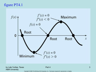
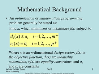
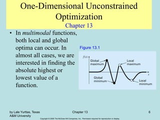
The document discusses optimization techniques for finding the minimum or maximum of a function. It explains that optimization involves searching for an extreme point of a function, unlike root finding which searches for where a function is equal to zero. The document outlines different types of optimization problems and describes the golden section search and Newton's method for solving unconstrained optimization problems in one dimension.

1. Copyright © 2006 The McGraw-Hill Companies, Inc. Permission required for reproduction or display.
by Lale Yurttas, Texas
A&M University
Chapter 13 1
Chapter 13

2. Copyright © 2006 The McGraw-Hill Companies, Inc. Permission required for reproduction or display.
by Lale Yurttas, Texas
A&M University
Part 4 2
Optimization
Part 4
• Root finding and optimization are related, both
involve guessing and searching for a point on a
function.
• Fundamental difference is:
– Root finding is searching for zeros of a function or
functions
– Optimization is finding the minimum or the
maximum of a function of several variables.

3. Copyright © 2006 The McGraw-Hill Companies, Inc. Permission required for reproduction or display.
by Lale Yurttas, Texas
A&M University
Part 4 3
figure PT4.1

4. Copyright © 2006 The McGraw-Hill Companies, Inc. Permission required for reproduction or display.
by Lale Yurttas, Texas
A&M University
Part 4 4
Mathematical Background
• An optimization or mathematical programming
problem generally be stated as:
Find x, which minimizes or maximizes f(x) subject to
*
,
,
2
,
1
)
(
*
,
,
2
,
1
)
(
p
i
b
x
e
m
i
a
x
d
i
i
i
i






Where x is an n-dimensional design vector, f(x) is
the objective function, di(x) are inequality
constraints, ei(x) are equality constraints, and ai
and bi are constants

5. Copyright © 2006 The McGraw-Hill Companies, Inc. Permission required for reproduction or display.
by Lale Yurttas, Texas
A&M University
Part 4 5
• Optimization problems can be classified on the
basis of the form of f(x):
– If f(x) and the constraints are linear, we have linear
programming.
– If f(x) is quadratic and the constraints are linear,
we have quadratic programming.
– If f(x) is not linear or quadratic and/or the
constraints are nonlinear, we have nonlinear
programming.
• When equations(*) are included, we have a
constrained optimization problem; otherwise,
it is unconstrained optimization problem.

6. Copyright © 2006 The McGraw-Hill Companies, Inc. Permission required for reproduction or display.
by Lale Yurttas, Texas
A&M University
Chapter 13 6
One-Dimensional Unconstrained
Optimization
Chapter 13
• In multimodal functions,
both local and global
optima can occur. In
almost all cases, we are
interested in finding the
absolute highest or
lowest value of a
function.
Figure 13.1

7. Copyright © 2006 The McGraw-Hill Companies, Inc. Permission required for reproduction or display.
by Lale Yurttas, Texas
A&M University
Chapter 13 7
How do we distinguish global optimum
from local one?
• By graphing to gain insight into the behavior
of the function.
• Using randomly generated starting guesses and
picking the largest of the optima as global.
• Perturbing the starting point to see if the
routine returns a better point or the same local
minimum.

8. Copyright © 2006 The McGraw-Hill Companies, Inc. Permission required for reproduction or display.
by Lale Yurttas, Texas
A&M University
Chapter 13 8
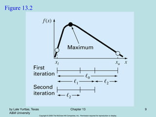
Golden-Section Search
• A unimodal function has a single maximum or a
minimum in the a given interval. For a unimodal
function:
– First pick two points that will bracket your extremum [xl,
xu].
– Pick an additional third point within this interval to
determine whether a maximum occurred.
– Then pick a fourth point to determine whether the
maximum has occurred within the first three or last three
points
– The key is making this approach efficient by choosing
intermediate points wisely thus minimizing the function
evaluations by replacing the old values with new values.

9. Copyright © 2006 The McGraw-Hill Companies, Inc. Permission required for reproduction or display.
by Lale Yurttas, Texas
A&M University
Chapter 13 9
Figure 13.2

10. Copyright © 2006 The McGraw-Hill Companies, Inc. Permission required for reproduction or display.
by Lale Yurttas, Texas
A&M University
Chapter 13 10
1
2
0
1
2
1
0
l
l
l
l
l
l
l



•The first condition specifies that the sum of the
two sub lengths l1 and l2 must equal the original
interval length.
•The second say that the ratio of the length must be
equal
61803
.
0
2
1
5
2
)
1
(
4
1
1
0
1
1
1 2
1
2
1
2
2
1
1
















R
R
R
R
R
l
l
R
l
l
l
l
l
Golden Ratio

11. Copyright © 2006 The McGraw-Hill Companies, Inc. Permission required for reproduction or display.
by Lale Yurttas, Texas
A&M University
Chapter 13 11
Figure 13.4

12. Copyright © 2006 The McGraw-Hill Companies, Inc. Permission required for reproduction or display.
by Lale Yurttas, Texas
A&M University
Chapter 13 12
The method starts with two initial guesses, xl and xu,
that bracket one local extremum of f(x):
• Next two interior points x1 and x2 are chosen according
to the golden ratio
d
x
x
d
x
x
x
x
d
u
l
l
u







2
1
)
(
2
1
5
• The function is evaluated at these two interior points.

13. Copyright © 2006 The McGraw-Hill Companies, Inc. Permission required for reproduction or display.
by Lale Yurttas, Texas
A&M University
Chapter 13 13
Two results can occur:
• If f(x1)>f(x2) then the domain of x to the left of x2 from xl to x2,
can be eliminated because it does not contain the maximum.
Then, x2 becomes the new xl for the next round.
• If f(x2)>f(x1), then the domain of x to the right of x1 from xl to x2,
would have been eliminated. In this case, x1 becomes the new xu
for the next round.
• New x1 is determined as before
)
(
2
1
5
1 l
u
l x
x
x
x 




14. Copyright © 2006 The McGraw-Hill Companies, Inc. Permission required for reproduction or display.
by Lale Yurttas, Texas
A&M University
Chapter 13 14
• The real benefit from the use of golden ratio is
because the original x1 and x2 were chosen
using golden ratio, we do not need to
recalculate all the function values for the next
iteration.

15. Copyright © 2006 The McGraw-Hill Companies, Inc. Permission required for reproduction or display.
by Lale Yurttas, Texas
A&M University
Chapter 13 15
Newton’s Method
• A similar approach to Newton- Raphson method can
be used to find an optimum of f(x) by defining a new
function g(x)=f‘(x). Thus because the same optimal
value x* satisfies both
f‘(x*)=g(x*)=0
We can use the following as a technique to the
extremum of f(x).
)
(
)
(
1
i
i
i
i
x
f
x
f
x
x





