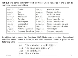
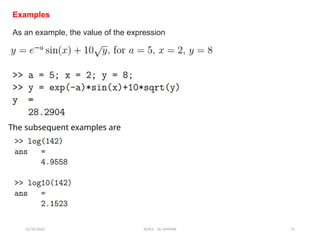
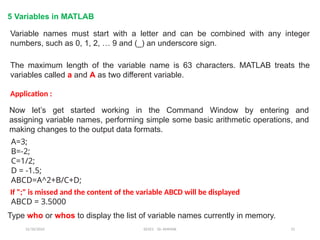
University of M’hamed BOUGARA of Boumerdes
Institute of Electrical and Electronics Engineering
(IGEE ex-INELEC)
Department of Power and Control engineering
Chapter 0: Introduction, Getting start with MATLAB
Dr. A. AMMAR
EE421 – Computation and Simulation using MATLAB /Simulink
12/10/2024 EE421 Dr. AMMAR 1
12/10/2024 EE421 Dr. AMMAR 2
1. Chapter 1: Introduction to use of MATLAB: elementary operations, operators,
functions.
2. Chapter 2 : Matrix computations and linear algebra.
3. Chapter 3 : programming, curve fitting and visualization
4. Chapter 4 : Introduction to use of SIMULINK with power system toolbox
5. Chapter 5: Embedding S-function in Simulink
6. Chapter5 : File I/O, building GUIs.
Module Outlines:
12/10/2024 EE421 Dr. AMMAR 3
Chapter 0: Introduction, Getting start with MATLAB
1. MATLAB interface presentation
2. Working in the Command Window
3. Using MATLAB as a calculator
4. Different MATLAB files extensions
5. Variables in MATLAB
6. M-File and MLX-Editors
7. Basic plotting
8. Summary
9. 9Quitting MATLAB
12/10/2024 EE421 Dr. AMMAR 4
Introduction: Getting start with MATLAB
The MATLAB package is employed in wide ranges of engineering and scientific
computing applications and is associated with the dynamic system simulation
package called Simulink
MATLAB’s interface and windows are customizable. Users can easily manipulate,
customize, and change preferences of the package according to their needs.
12/10/2024 EE421 Dr. AMMAR 5
Fig.1 shows the default main window of MATLAB 2017b. It must be noted
that the interface menu and tools have changed over the years in an effort to
make the package more user friendly and the tools more intuitive.
Current path
Current Folder
Command Window
1 MATLAB interface presentation
Fig.1
12/10/2024 EE421 Dr. AMMAR 6
The default window has the main menu tools, a Current Directory indicator, and
Command, Workspace, and Command History windows.
The main components of the user interface tools are as follows:
Tools and toolbars are grouped into three menus HOME, PLOTS,
and APPs (see Fig.2).
The HOME tab contains all the main tools.
It’s where you can create and delete new files and variables, import data, access
the code analyzer, launch Simulink, and access addons and help options…etc
Fig.2
12/10/2024 EE421 Dr. AMMAR 7
• The Command Window is in the central pane (by default). All commands and/or
(small) scripts/codes can be entered directly.
• The Workspace pane (Fig.3) of the default desktop window shows the current
entries and saved variables during the session. These entries are saved
temporarily until the MATLAB application is closed. All essential attributes and
properties of entries/variables (variable names, values, and types) are displayed
in the workspace.
Fig.3
12/10/2024 EE421 Dr. AMMAR 8
2 Working in the Command Window
Work in MATLAB generally starts in the Command Window, but before you type any
command, it is worth noting the current directory. The current directory address can
be viewed directly from the main window (see Fig.4).
or by typing this command in the
Command Window:
>> pwd
For short commands and calculations and/or to view attributes of the available
variables in the current directory, use the Command Window.
However, for series of commands and longer scripts, it is more efficient to use
script editors, such as the M-file and MLX-file editors.
Fig.4
12/10/2024 EE421 Dr. AMMAR 9
Command Window generally used for:
Use the Command Window in these instances:
• To perform short calculations
• To view error and warning messages from commands or/and after executing M-files,
MLX-files, and SLX/MDL Simulink models
• To view variable attributes saved in the workspace and files in the
current directory
• To view the contents of MATLAB compatible files
• To execute MATLAB files, such as M-files, MLX-files, SLX/MDL-files,
and MAT-files
• To get hands-on, quick help with MATLAB commands/functions and user-created
function files
• To make adjustments to the display formats of numerical data
• To add/remove a path/directory
• To create/delete/save variables and files
12/10/2024 EE421 Dr. AMMAR 10
3 Using MATLAB as a calculator
As an example of a simple interactive calculation, just type the expression you
want to evaluate. Let’s start at the very beginning. For example, let’s suppose you
want to calculate the expression, 1 + 2 × 3.
You type it at the prompt command (>>) as follows,
MATLAB uses a default variable ans, short for answer, to store the results of the
current calculation.
To avoid this, you may assign a value to a variable or output argument name. For
example
12/10/2024 EE421 Dr. AMMAR 11
Table 1 gives the partial list of arithmetic operators.
Mathematical functions
MATLAB offers many predefined mathematical functions for technical computing
which contains a large set of mathematical functions.
Typing help elfun and help specfun calls up full lists of elementary and special
functions respectively
There is a long list of mathematical functions that are built into MATLAB. These
functions are called built-ins. Many standard mathematical functions, such as sin(x),
cos(x), tan(x), ex
, ln(x), are evaluated by the functions sin, cos, tan, exp, and log
respectively in MATLAB.
12/10/2024 EE421 Dr. AMMAR 12
Table.2 lists some commonly used functions, where variables x and y can be
numbers, vectors, or matrices.
In addition to the elementary functions, MATLAB includes a number of predefined
constant values. Table.3 shows of the most common values is given in the
following Table
12/10/2024 EE421 Dr. AMMAR 13
Examples
As an example, the value of the expression
The subsequent examples are
12/10/2024 EE421 Dr. AMMAR 14
The MATLAB application has a few files that are recognizable by their extensions.
They are .M, .MLX, .MAT, .BI, and .FIG.
M-files are used to write programs/scripts/function files.
MAT-files are used to save all types of variables available in the workspace and can
be accessed easily from M/MLX-files and the Command Window
.FIG files are used to save figure windows in MATLAB.
In addition, the Simulink application has three types of files .mdl, .slx, and .slxc.
They are used to build and simulate Simulink models
4 Different MATLAB files extensions
12/10/2024 EE421 Dr. AMMAR 15
5 Variables in MATLAB
Variable names must start with a letter and can be combined with any integer
numbers, such as 0, 1, 2, … 9 and (_) an underscore sign.
The maximum length of the variable name is 63 characters. MATLAB treats the
variables called a and A as two different variable.
Application :
Now let’s get started working in the Command Window by entering and
assigning variable names, performing simple some basic arithmetic operations, and
making changes to the output data formats.
A=3;
B=-2;
C=1/2;
D = -1.5;
ABCD=A^2+B/C+D;
If ";" is missed and the content of the variable ABCD will be displayed
ABCD = 3.5000
Type who or whos to display the list of variable names currently in memory.
12/10/2024 EE421 Dr. AMMAR 16
>> sqrt(ABCD)
ans = 1.8708
ABCD = 3.5000
>> format bank
>> ABCD
ABCD =
3.50
>> format long eng
>> ABCD
ABCD =
3.50000000000000e+000
While all computations in MATLAB are done in double precision, the default format
prints results with five significant digits. The format of the displayed output can be
displayed using different format, such as format long, format short, format long
eng, format bank, format hexadecimal, format rational, etc.
12/10/2024 EE421 Dr. AMMAR 17
MATLAB Command Display
format Default. Same as format short
format short Scaled fixed point format with 5 digits
format long Scaled fixed point format with 15 digits
format short e Floating point format with 5 digits
format long e Floating point format with 15 digits
format short g Best of fixed or floating point with 5 digits
format long g Best of fixed or floating point with 15 digits
format hex Hexadecimal format
format + The symbols +, - and blank are printed for positive, negative,
and zero elements
format bank Fixed format for dollars and cents
format rat Approximation by ratio of small integers
format compact Suppress extra line feeds
format loose Puts the extra line feeds back in
The following table (Table.4) show the different formats and their display
12/10/2024 EE421 Dr. AMMAR 18
Character Variables
A sequence of characters in single quotes is called a character string or text variable
Results in
A text variable can be augmented with more text variables, for example
produces
12/10/2024 EE421 Dr. AMMAR 19
Another useful feature of the Command Window is using the keyboard’s up-
arrow (↑) to recall previously typed variables or commands.
The values and attributes of all variables entered in the Command Window will
be saved in the workspace until you clean up the workspace by deleting the
variables using the clear, clearvars, or clear all command
clc for cleaning up the Command Window and starting with a blank Command
Window
12/10/2024 EE421 Dr. AMMAR 20
Different Variables and Data Sets in
MATLAB
MATLAB supports several different data types—numeric, character, logical, table,
cell, structure, and function handle. Note that the function handle can also take
vectors (row or column vectors), not only scalar numbers.
Let’s look at several examples on Fig.5 of how to generate various data types
supported in MATLAB:
• Numerical data
• Logical arrays
• Character arrays/variables
• Table arrays
• Cell arrays
• Structure arrays
• Function handles
• Classes and graphic handles
Fig.5
12/10/2024 EE421 Dr. AMMAR 21
In general it is clear that MATLAB reads every entry as an array/ matrix. For
example, scalar is read by MATLAB as an array of size 1-by-1.
This attribute of MATLAB is logically linked to its name, MATrix LABoratory.
MATLAB’s default storage (memory allocation) is double precision, which is the
maximum available space allocated.
However, for memory efficiency and faster calculation purposes, other storage
formats can also be used. MATLAB supports single precision or integer type and
int8 … 64, uint8 …64 storage format types.
Table.5 shows how data can be saved in every storage class type and the
conversion function used in MATLAB for each type.
12/10/2024 EE421 Dr. AMMAR 22
Fig.6 shows all the data storage types and data formats supported in MATLAB.
12/10/2024 EE421 Dr. AMMAR 23
6 M-File and MLX–File Editors
In the previous examples, all of the operations and work are done in the Command
Window. However, for programming and writing, editing and debugging, M-file and
MLX-file editors will be of great help due to their helpful tools and hints in writing fast
and more efficient codes/scripts/programs.
The overall functionality of M-files and MLX-files is similar except for one important
feature. The MLX file editor window can display the outputs of
calculations/simulations within the MLX editor window and indicate the most
common command syntax related errors on its left-side output window.
The M-file editor shows all errors in the Command Window after the M-file’s
execution. The M-file editor toolbar is shown in Fig.7
M-File Editor
We can push new script to open the M-file editor
Fig.7
12/10/2024 EE421 Dr. AMMAR 24
In the M-file editor’s main tools menu is shown in Fig. it is sub-grouped in three
tabs EDITOR, PUBLISH, and VIEW, as shown in Fig.8
In order to demonstrate some of the highlighted tools and options of the M-file.
let’s look at the following example
First, the solution script of this simple example will created in the M-file editor
12/10/2024 EE421 Dr. AMMAR 25
The algorithm for solving this example will be done in the following steps of
the following six steps.
1. Insert some comments describing the given problem statement.
2. Define the input variable:
3. Perform the computation:
4. Plot the simulation results: α vs. F(α).
% Step 1. Problem statement
% Pythagorean Theorem: F = 1 - (sin^2 (alpha)+cos^2(alpha));
% Input variable: alpha = -0.5*pi ... 0.5*pi
% Step 2. Define the input variable
alpha = -pi/2:pi/100:pi/2;
% Step 3. Perform the computation
F = 1-(sin(alpha).^2+cos(alpha).^2);
% Step 5. Plot the simulation results: alpha vs. F(alpha)
plot(alpha,F)
legend('alpha vs F(alpha)', 'F(alpha) = 0')
title('Simulation of MATLAB"s precision via the Pythagorean Theorem '),
grid on
xlabel('alpha'), ylabel('F(alpha) = 1-(sin(alpha)^2+cos(alpha)^2)')
12/10/2024 EE421 Dr. AMMAR 26
% Comments
Comments are not executable and contain additional information for the users. The
% sign is used to place comments and remarks or any additional information within
M-files and MLX-files.
Moreover, inserting %% at the beginning of a line and leaving a blank space after
it creates a cell mode in the script.
12/10/2024 EE421 Dr. AMMAR 27
After writing the script in the editor, save the M-file with a valid filename
(example1.m).
Now, to publish it as an HTML format, press the Publish button under
the PUBLISH
Tab. After pressing the button, the script is executed automatically and its
HTML-formatted report will be generated, as shown in Fig.
12/10/2024 EE421 Dr. AMMAR 28
7 Basic plotting
MATLAB’s extensive, device-independent plotting capabilities are one of its most
powerful features. They make it very easy to plot any data at any time. To plot a
data set, just create two vectors containing the x and y values to be plotted, and
use the plot function.
For example, suppose that we wish to plot the function
For values of x between 0 and 10.
The first statement creates a vector of x values between 0 and 10 using the colon
operator.
x=0:1:10;
y = x^2 – 10*x + 15
The second statement calculates the y values from the equation
Finally, the third statement creates the plot.
plot(x,y);
12/10/2024 EE421 Dr. AMMAR 29
When the plot function is executed, MATLAB opens a Figure Window and displays
the plot in that window. The plot produced by these statements is shown in Fig.9
As we just saw, plotting is very easy in MATLAB. Any pair of vectors can be plotted
versus each other as long as both vectors have the same length.
However, the result is not a finished product, since there are no titles, axis labels, or
grid lines on the plot.
Fig.9
12/10/2024 EE421 Dr. AMMAR 30
Titles and axis labels can be added to a plot with the title, xlabel, and ylabel
functions.
Grid lines can be added or removed from the plot with the grid command: grid on
turns on grid lines, and grid off turns off grid lines.
For example, the following statements generate a plot of the function
with titles, labels, and grid lines.
x = 0:1:10;
y = x.^2 – 10.*x + 15;
plot(x,y);
title ('Plot of y = x.^2 – 10.*x + 15');
xlabel ('x');
ylabel ('y');
grid on;
12/10/2024 EE421 Dr. AMMAR 31
Otherwise, we can use the property editor (Fig.10), in View Menu
Fig.10
12/10/2024 EE421 Dr. AMMAR 32
In addition, the “File/Save As” menu option in the Figure Window can be used
to save a plot as a graphical image. In this case, the user selects the filename and
the type of image from a standard dialog box (Fig.11).
Fig.11
12/10/2024 EE421 Dr. AMMAR 33
MATLAB allows a programmer to select the color of a line to be plotted, the style of
the line to be plotted, and the type of marker to be used for data points on the line.
These traits may be selected by adding an extra argument called LineSpec to the
The character array can have up to three characters, with the first character
specifying the color of the line, the second character specifying the style of the
marker, and the last character specifying the style of the line.
12/10/2024 EE421 Dr. AMMAR 34
Table.6 shows All possible Plot Colors, Marker Styles,
and Line Styles
Note that all plotting option can be done also using the property editor
Table .6
12/10/2024 EE421 Dr. AMMAR 35
8. Summary
This chapter introduced the MATLAB environment, including its settings, variables,
common commands, and M-file tools. You also learned about assigning variables
and values from the Command Window and working in the M-file editor windows,
Finally we’ve seen some plotting options
The following summary lists all of the MATLAB special symbols, commands, and
functions described in this chapter, along with a brief description of each one.
12/10/2024 EE421 Dr. AMMAR 36
12/10/2024 EE421 Dr. AMMAR 37
12/10/2024 EE421 Dr. AMMAR 38
9. Quitting MATLAB
To end your MATLAB session, type quit in the Command Window, or select
File>Exit MATLAB in the desktop main menu.
12/10/2024 EE421 Dr. AMMAR 39
Recommended Textbooks

Chap#0_Introducation_to_nsnsnnMATLAB.pptx

  • 1.
    University of M’hamedBOUGARA of Boumerdes Institute of Electrical and Electronics Engineering (IGEE ex-INELEC) Department of Power and Control engineering Chapter 0: Introduction, Getting start with MATLAB Dr. A. AMMAR EE421 – Computation and Simulation using MATLAB /Simulink 12/10/2024 EE421 Dr. AMMAR 1
  • 2.
    12/10/2024 EE421 Dr.AMMAR 2 1. Chapter 1: Introduction to use of MATLAB: elementary operations, operators, functions. 2. Chapter 2 : Matrix computations and linear algebra. 3. Chapter 3 : programming, curve fitting and visualization 4. Chapter 4 : Introduction to use of SIMULINK with power system toolbox 5. Chapter 5: Embedding S-function in Simulink 6. Chapter5 : File I/O, building GUIs. Module Outlines:
  • 3.
    12/10/2024 EE421 Dr.AMMAR 3 Chapter 0: Introduction, Getting start with MATLAB 1. MATLAB interface presentation 2. Working in the Command Window 3. Using MATLAB as a calculator 4. Different MATLAB files extensions 5. Variables in MATLAB 6. M-File and MLX-Editors 7. Basic plotting 8. Summary 9. 9Quitting MATLAB
  • 4.
    12/10/2024 EE421 Dr.AMMAR 4 Introduction: Getting start with MATLAB The MATLAB package is employed in wide ranges of engineering and scientific computing applications and is associated with the dynamic system simulation package called Simulink MATLAB’s interface and windows are customizable. Users can easily manipulate, customize, and change preferences of the package according to their needs.
  • 5.
    12/10/2024 EE421 Dr.AMMAR 5 Fig.1 shows the default main window of MATLAB 2017b. It must be noted that the interface menu and tools have changed over the years in an effort to make the package more user friendly and the tools more intuitive. Current path Current Folder Command Window 1 MATLAB interface presentation Fig.1
  • 6.
    12/10/2024 EE421 Dr.AMMAR 6 The default window has the main menu tools, a Current Directory indicator, and Command, Workspace, and Command History windows. The main components of the user interface tools are as follows: Tools and toolbars are grouped into three menus HOME, PLOTS, and APPs (see Fig.2). The HOME tab contains all the main tools. It’s where you can create and delete new files and variables, import data, access the code analyzer, launch Simulink, and access addons and help options…etc Fig.2
  • 7.
    12/10/2024 EE421 Dr.AMMAR 7 • The Command Window is in the central pane (by default). All commands and/or (small) scripts/codes can be entered directly. • The Workspace pane (Fig.3) of the default desktop window shows the current entries and saved variables during the session. These entries are saved temporarily until the MATLAB application is closed. All essential attributes and properties of entries/variables (variable names, values, and types) are displayed in the workspace. Fig.3
  • 8.
    12/10/2024 EE421 Dr.AMMAR 8 2 Working in the Command Window Work in MATLAB generally starts in the Command Window, but before you type any command, it is worth noting the current directory. The current directory address can be viewed directly from the main window (see Fig.4). or by typing this command in the Command Window: >> pwd For short commands and calculations and/or to view attributes of the available variables in the current directory, use the Command Window. However, for series of commands and longer scripts, it is more efficient to use script editors, such as the M-file and MLX-file editors. Fig.4
  • 9.
    12/10/2024 EE421 Dr.AMMAR 9 Command Window generally used for: Use the Command Window in these instances: • To perform short calculations • To view error and warning messages from commands or/and after executing M-files, MLX-files, and SLX/MDL Simulink models • To view variable attributes saved in the workspace and files in the current directory • To view the contents of MATLAB compatible files • To execute MATLAB files, such as M-files, MLX-files, SLX/MDL-files, and MAT-files • To get hands-on, quick help with MATLAB commands/functions and user-created function files • To make adjustments to the display formats of numerical data • To add/remove a path/directory • To create/delete/save variables and files
  • 10.
    12/10/2024 EE421 Dr.AMMAR 10 3 Using MATLAB as a calculator As an example of a simple interactive calculation, just type the expression you want to evaluate. Let’s start at the very beginning. For example, let’s suppose you want to calculate the expression, 1 + 2 × 3. You type it at the prompt command (>>) as follows, MATLAB uses a default variable ans, short for answer, to store the results of the current calculation. To avoid this, you may assign a value to a variable or output argument name. For example
  • 11.
    12/10/2024 EE421 Dr.AMMAR 11 Table 1 gives the partial list of arithmetic operators. Mathematical functions MATLAB offers many predefined mathematical functions for technical computing which contains a large set of mathematical functions. Typing help elfun and help specfun calls up full lists of elementary and special functions respectively There is a long list of mathematical functions that are built into MATLAB. These functions are called built-ins. Many standard mathematical functions, such as sin(x), cos(x), tan(x), ex , ln(x), are evaluated by the functions sin, cos, tan, exp, and log respectively in MATLAB.
  • 12.
    12/10/2024 EE421 Dr.AMMAR 12 Table.2 lists some commonly used functions, where variables x and y can be numbers, vectors, or matrices. In addition to the elementary functions, MATLAB includes a number of predefined constant values. Table.3 shows of the most common values is given in the following Table
  • 13.
    12/10/2024 EE421 Dr.AMMAR 13 Examples As an example, the value of the expression The subsequent examples are
  • 14.
    12/10/2024 EE421 Dr.AMMAR 14 The MATLAB application has a few files that are recognizable by their extensions. They are .M, .MLX, .MAT, .BI, and .FIG. M-files are used to write programs/scripts/function files. MAT-files are used to save all types of variables available in the workspace and can be accessed easily from M/MLX-files and the Command Window .FIG files are used to save figure windows in MATLAB. In addition, the Simulink application has three types of files .mdl, .slx, and .slxc. They are used to build and simulate Simulink models 4 Different MATLAB files extensions
  • 15.
    12/10/2024 EE421 Dr.AMMAR 15 5 Variables in MATLAB Variable names must start with a letter and can be combined with any integer numbers, such as 0, 1, 2, … 9 and (_) an underscore sign. The maximum length of the variable name is 63 characters. MATLAB treats the variables called a and A as two different variable. Application : Now let’s get started working in the Command Window by entering and assigning variable names, performing simple some basic arithmetic operations, and making changes to the output data formats. A=3; B=-2; C=1/2; D = -1.5; ABCD=A^2+B/C+D; If ";" is missed and the content of the variable ABCD will be displayed ABCD = 3.5000 Type who or whos to display the list of variable names currently in memory.
  • 16.
    12/10/2024 EE421 Dr.AMMAR 16 >> sqrt(ABCD) ans = 1.8708 ABCD = 3.5000 >> format bank >> ABCD ABCD = 3.50 >> format long eng >> ABCD ABCD = 3.50000000000000e+000 While all computations in MATLAB are done in double precision, the default format prints results with five significant digits. The format of the displayed output can be displayed using different format, such as format long, format short, format long eng, format bank, format hexadecimal, format rational, etc.
  • 17.
    12/10/2024 EE421 Dr.AMMAR 17 MATLAB Command Display format Default. Same as format short format short Scaled fixed point format with 5 digits format long Scaled fixed point format with 15 digits format short e Floating point format with 5 digits format long e Floating point format with 15 digits format short g Best of fixed or floating point with 5 digits format long g Best of fixed or floating point with 15 digits format hex Hexadecimal format format + The symbols +, - and blank are printed for positive, negative, and zero elements format bank Fixed format for dollars and cents format rat Approximation by ratio of small integers format compact Suppress extra line feeds format loose Puts the extra line feeds back in The following table (Table.4) show the different formats and their display
  • 18.
    12/10/2024 EE421 Dr.AMMAR 18 Character Variables A sequence of characters in single quotes is called a character string or text variable Results in A text variable can be augmented with more text variables, for example produces
  • 19.
    12/10/2024 EE421 Dr.AMMAR 19 Another useful feature of the Command Window is using the keyboard’s up- arrow (↑) to recall previously typed variables or commands. The values and attributes of all variables entered in the Command Window will be saved in the workspace until you clean up the workspace by deleting the variables using the clear, clearvars, or clear all command clc for cleaning up the Command Window and starting with a blank Command Window
  • 20.
    12/10/2024 EE421 Dr.AMMAR 20 Different Variables and Data Sets in MATLAB MATLAB supports several different data types—numeric, character, logical, table, cell, structure, and function handle. Note that the function handle can also take vectors (row or column vectors), not only scalar numbers. Let’s look at several examples on Fig.5 of how to generate various data types supported in MATLAB: • Numerical data • Logical arrays • Character arrays/variables • Table arrays • Cell arrays • Structure arrays • Function handles • Classes and graphic handles Fig.5
  • 21.
    12/10/2024 EE421 Dr.AMMAR 21 In general it is clear that MATLAB reads every entry as an array/ matrix. For example, scalar is read by MATLAB as an array of size 1-by-1. This attribute of MATLAB is logically linked to its name, MATrix LABoratory. MATLAB’s default storage (memory allocation) is double precision, which is the maximum available space allocated. However, for memory efficiency and faster calculation purposes, other storage formats can also be used. MATLAB supports single precision or integer type and int8 … 64, uint8 …64 storage format types. Table.5 shows how data can be saved in every storage class type and the conversion function used in MATLAB for each type.
  • 22.
    12/10/2024 EE421 Dr.AMMAR 22 Fig.6 shows all the data storage types and data formats supported in MATLAB.
  • 23.
    12/10/2024 EE421 Dr.AMMAR 23 6 M-File and MLX–File Editors In the previous examples, all of the operations and work are done in the Command Window. However, for programming and writing, editing and debugging, M-file and MLX-file editors will be of great help due to their helpful tools and hints in writing fast and more efficient codes/scripts/programs. The overall functionality of M-files and MLX-files is similar except for one important feature. The MLX file editor window can display the outputs of calculations/simulations within the MLX editor window and indicate the most common command syntax related errors on its left-side output window. The M-file editor shows all errors in the Command Window after the M-file’s execution. The M-file editor toolbar is shown in Fig.7 M-File Editor We can push new script to open the M-file editor Fig.7
  • 24.
    12/10/2024 EE421 Dr.AMMAR 24 In the M-file editor’s main tools menu is shown in Fig. it is sub-grouped in three tabs EDITOR, PUBLISH, and VIEW, as shown in Fig.8 In order to demonstrate some of the highlighted tools and options of the M-file. let’s look at the following example First, the solution script of this simple example will created in the M-file editor
  • 25.
    12/10/2024 EE421 Dr.AMMAR 25 The algorithm for solving this example will be done in the following steps of the following six steps. 1. Insert some comments describing the given problem statement. 2. Define the input variable: 3. Perform the computation: 4. Plot the simulation results: α vs. F(α). % Step 1. Problem statement % Pythagorean Theorem: F = 1 - (sin^2 (alpha)+cos^2(alpha)); % Input variable: alpha = -0.5*pi ... 0.5*pi % Step 2. Define the input variable alpha = -pi/2:pi/100:pi/2; % Step 3. Perform the computation F = 1-(sin(alpha).^2+cos(alpha).^2); % Step 5. Plot the simulation results: alpha vs. F(alpha) plot(alpha,F) legend('alpha vs F(alpha)', 'F(alpha) = 0') title('Simulation of MATLAB"s precision via the Pythagorean Theorem '), grid on xlabel('alpha'), ylabel('F(alpha) = 1-(sin(alpha)^2+cos(alpha)^2)')
  • 26.
    12/10/2024 EE421 Dr.AMMAR 26 % Comments Comments are not executable and contain additional information for the users. The % sign is used to place comments and remarks or any additional information within M-files and MLX-files. Moreover, inserting %% at the beginning of a line and leaving a blank space after it creates a cell mode in the script.
  • 27.
    12/10/2024 EE421 Dr.AMMAR 27 After writing the script in the editor, save the M-file with a valid filename (example1.m). Now, to publish it as an HTML format, press the Publish button under the PUBLISH Tab. After pressing the button, the script is executed automatically and its HTML-formatted report will be generated, as shown in Fig.
  • 28.
    12/10/2024 EE421 Dr.AMMAR 28 7 Basic plotting MATLAB’s extensive, device-independent plotting capabilities are one of its most powerful features. They make it very easy to plot any data at any time. To plot a data set, just create two vectors containing the x and y values to be plotted, and use the plot function. For example, suppose that we wish to plot the function For values of x between 0 and 10. The first statement creates a vector of x values between 0 and 10 using the colon operator. x=0:1:10; y = x^2 – 10*x + 15 The second statement calculates the y values from the equation Finally, the third statement creates the plot. plot(x,y);
  • 29.
    12/10/2024 EE421 Dr.AMMAR 29 When the plot function is executed, MATLAB opens a Figure Window and displays the plot in that window. The plot produced by these statements is shown in Fig.9 As we just saw, plotting is very easy in MATLAB. Any pair of vectors can be plotted versus each other as long as both vectors have the same length. However, the result is not a finished product, since there are no titles, axis labels, or grid lines on the plot. Fig.9
  • 30.
    12/10/2024 EE421 Dr.AMMAR 30 Titles and axis labels can be added to a plot with the title, xlabel, and ylabel functions. Grid lines can be added or removed from the plot with the grid command: grid on turns on grid lines, and grid off turns off grid lines. For example, the following statements generate a plot of the function with titles, labels, and grid lines. x = 0:1:10; y = x.^2 – 10.*x + 15; plot(x,y); title ('Plot of y = x.^2 – 10.*x + 15'); xlabel ('x'); ylabel ('y'); grid on;
  • 31.
    12/10/2024 EE421 Dr.AMMAR 31 Otherwise, we can use the property editor (Fig.10), in View Menu Fig.10
  • 32.
    12/10/2024 EE421 Dr.AMMAR 32 In addition, the “File/Save As” menu option in the Figure Window can be used to save a plot as a graphical image. In this case, the user selects the filename and the type of image from a standard dialog box (Fig.11). Fig.11
  • 33.
    12/10/2024 EE421 Dr.AMMAR 33 MATLAB allows a programmer to select the color of a line to be plotted, the style of the line to be plotted, and the type of marker to be used for data points on the line. These traits may be selected by adding an extra argument called LineSpec to the The character array can have up to three characters, with the first character specifying the color of the line, the second character specifying the style of the marker, and the last character specifying the style of the line.
  • 34.
    12/10/2024 EE421 Dr.AMMAR 34 Table.6 shows All possible Plot Colors, Marker Styles, and Line Styles Note that all plotting option can be done also using the property editor Table .6
  • 35.
    12/10/2024 EE421 Dr.AMMAR 35 8. Summary This chapter introduced the MATLAB environment, including its settings, variables, common commands, and M-file tools. You also learned about assigning variables and values from the Command Window and working in the M-file editor windows, Finally we’ve seen some plotting options The following summary lists all of the MATLAB special symbols, commands, and functions described in this chapter, along with a brief description of each one.
  • 36.
  • 37.
  • 38.
    12/10/2024 EE421 Dr.AMMAR 38 9. Quitting MATLAB To end your MATLAB session, type quit in the Command Window, or select File>Exit MATLAB in the desktop main menu.
  • 39.
    12/10/2024 EE421 Dr.AMMAR 39 Recommended Textbooks