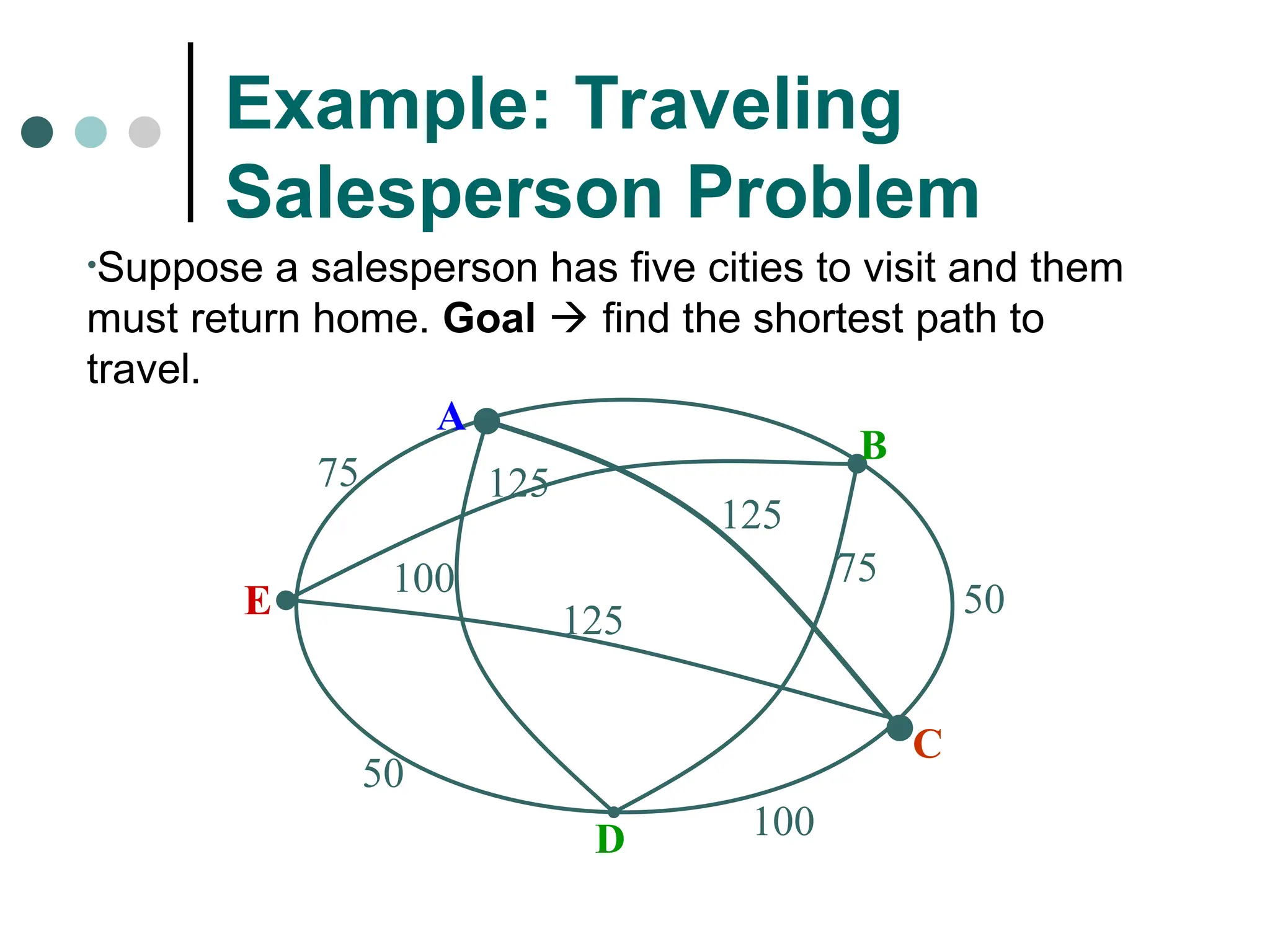
Ch4: Searching Techniques
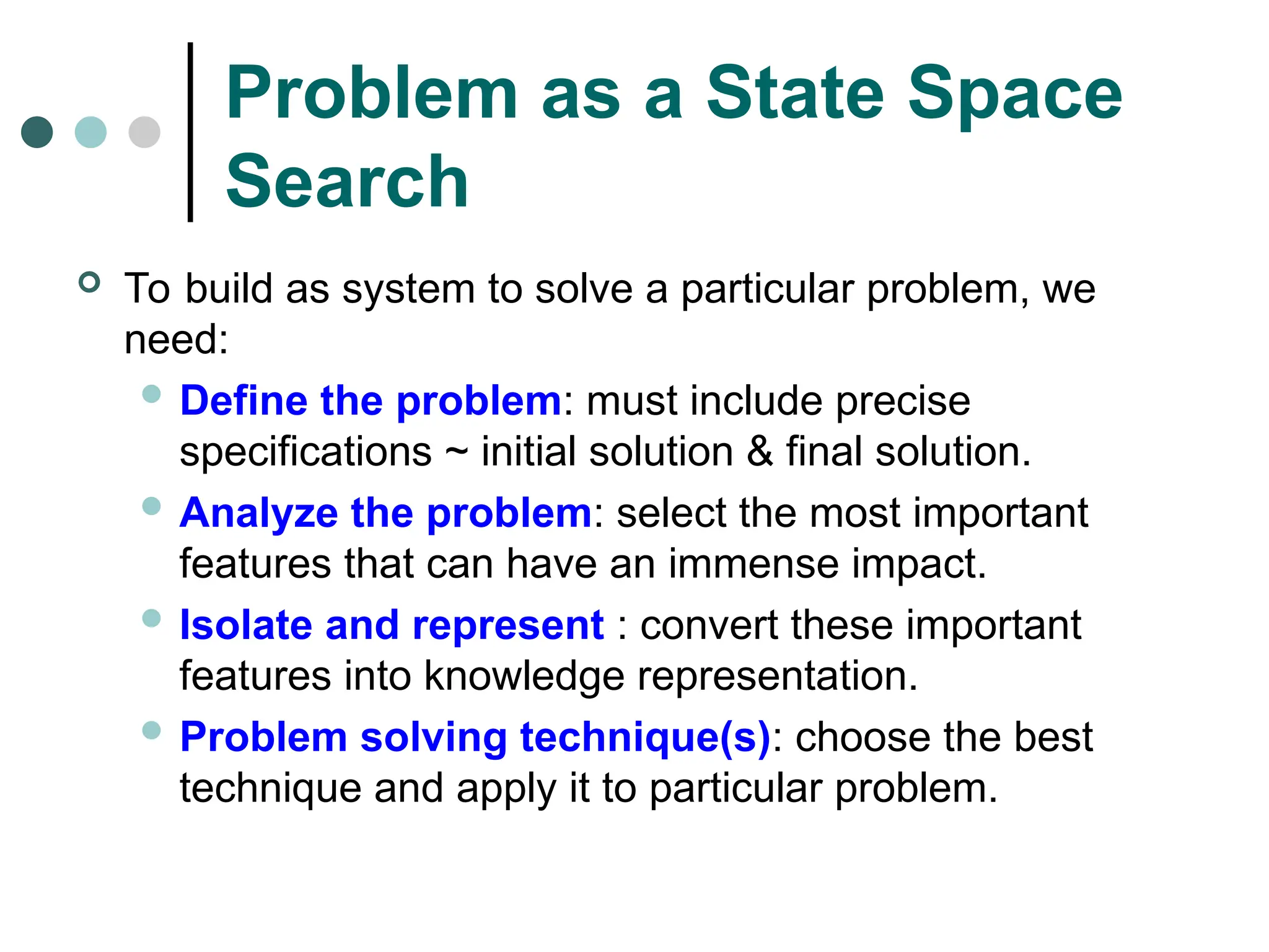
Define the problem: must include precise specifications ~ initial solution & final solution.
Analyze the problem: select the most important features that can have an immense impact.
Isolate and represent : convert these important features into knowledge representation.
Problem solving technique(s): choose the best technique and apply it to particular problem.
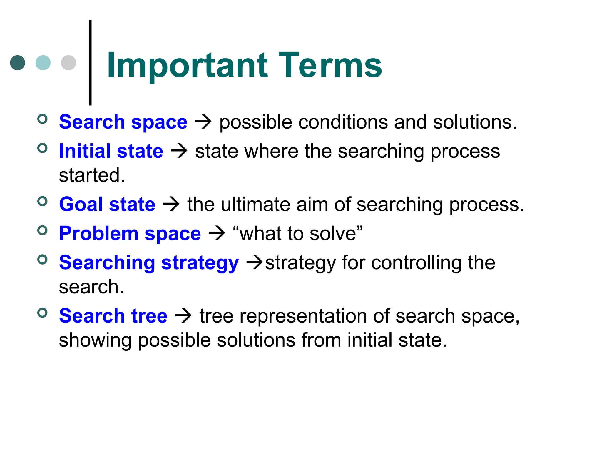
Search space possible conditions and solutions.
Initial state state where the searching process started.
Goal state the ultimate aim of searching process.
Problem space “what to solve”
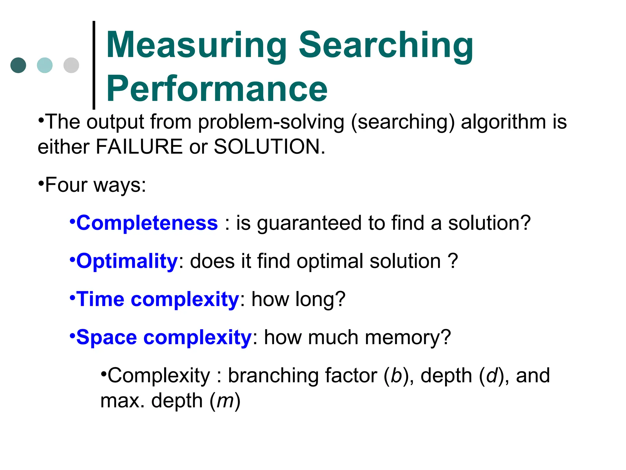
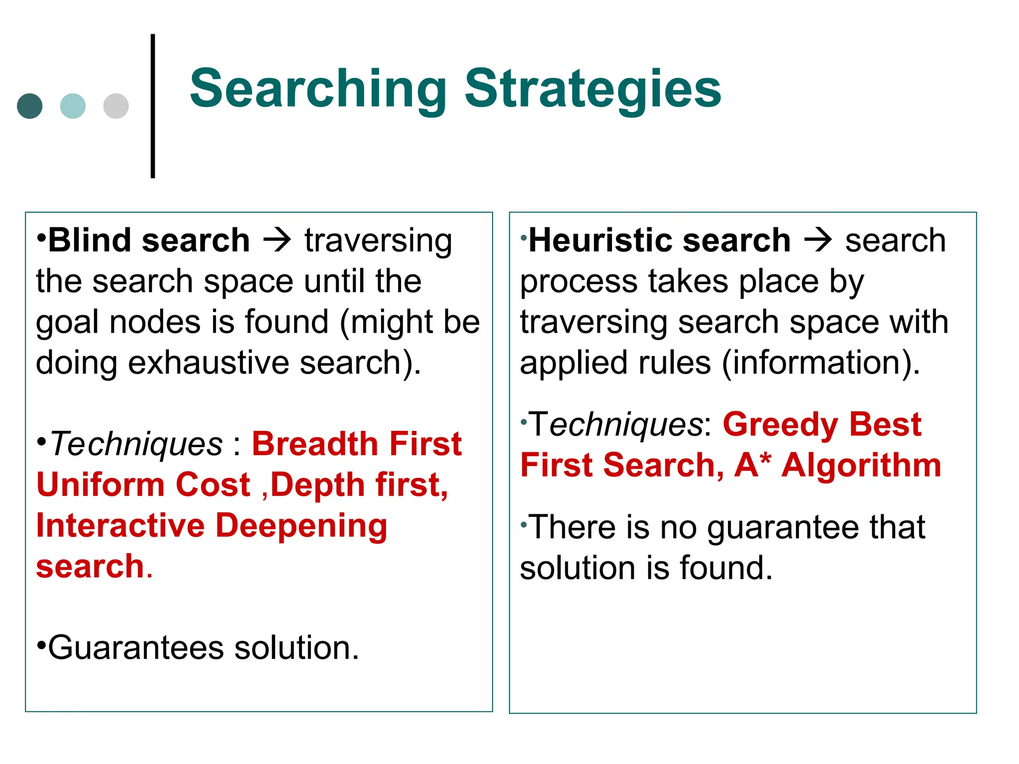
Searching strategy strategy for controlling the search.
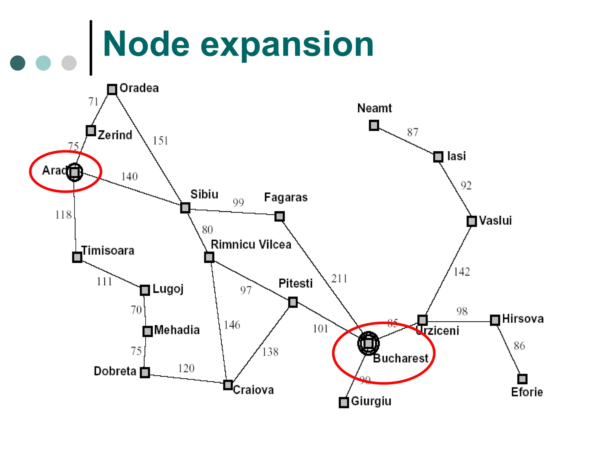
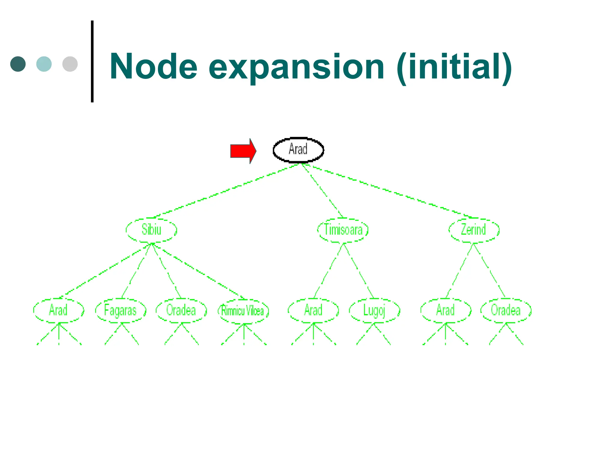
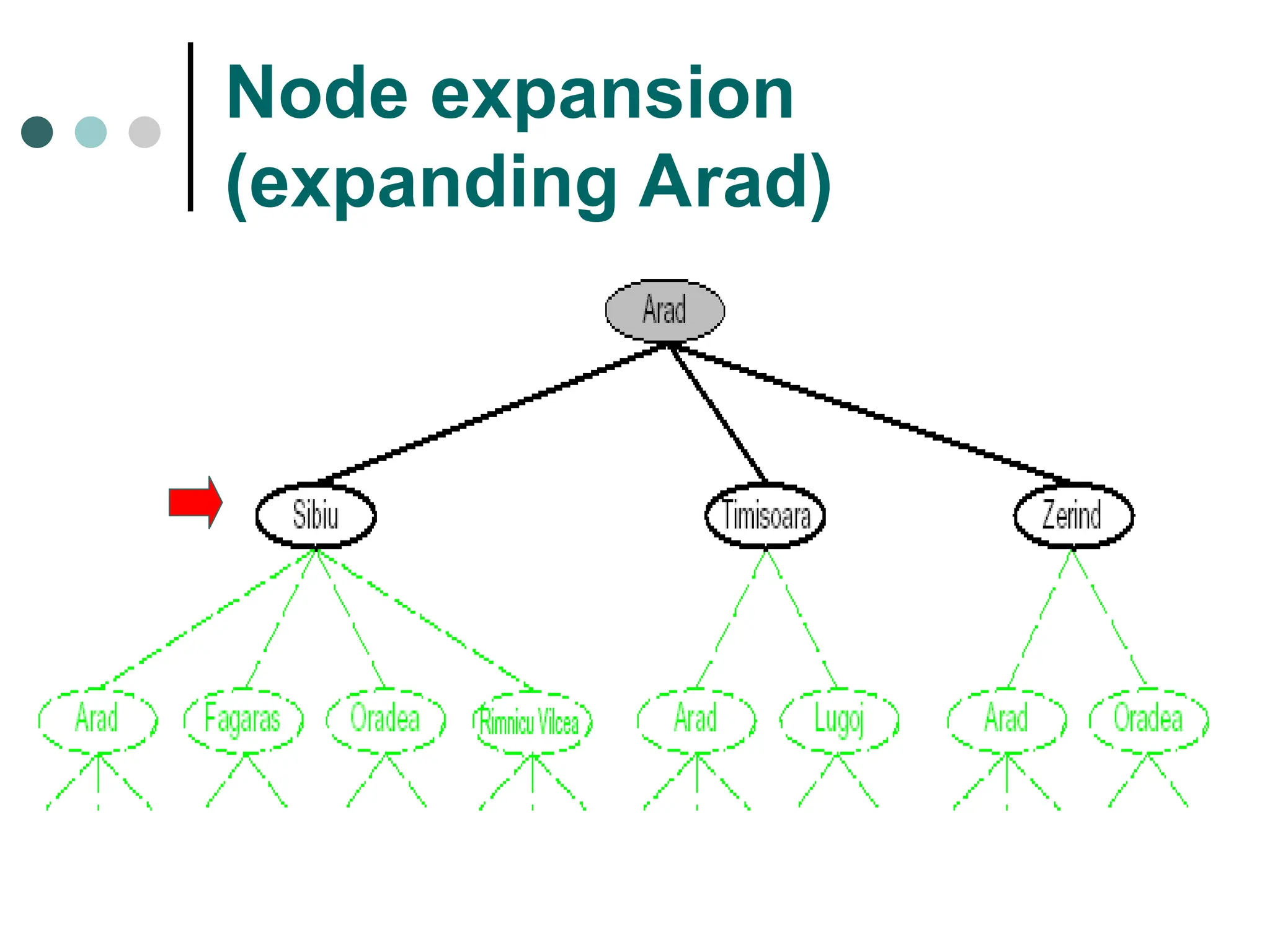
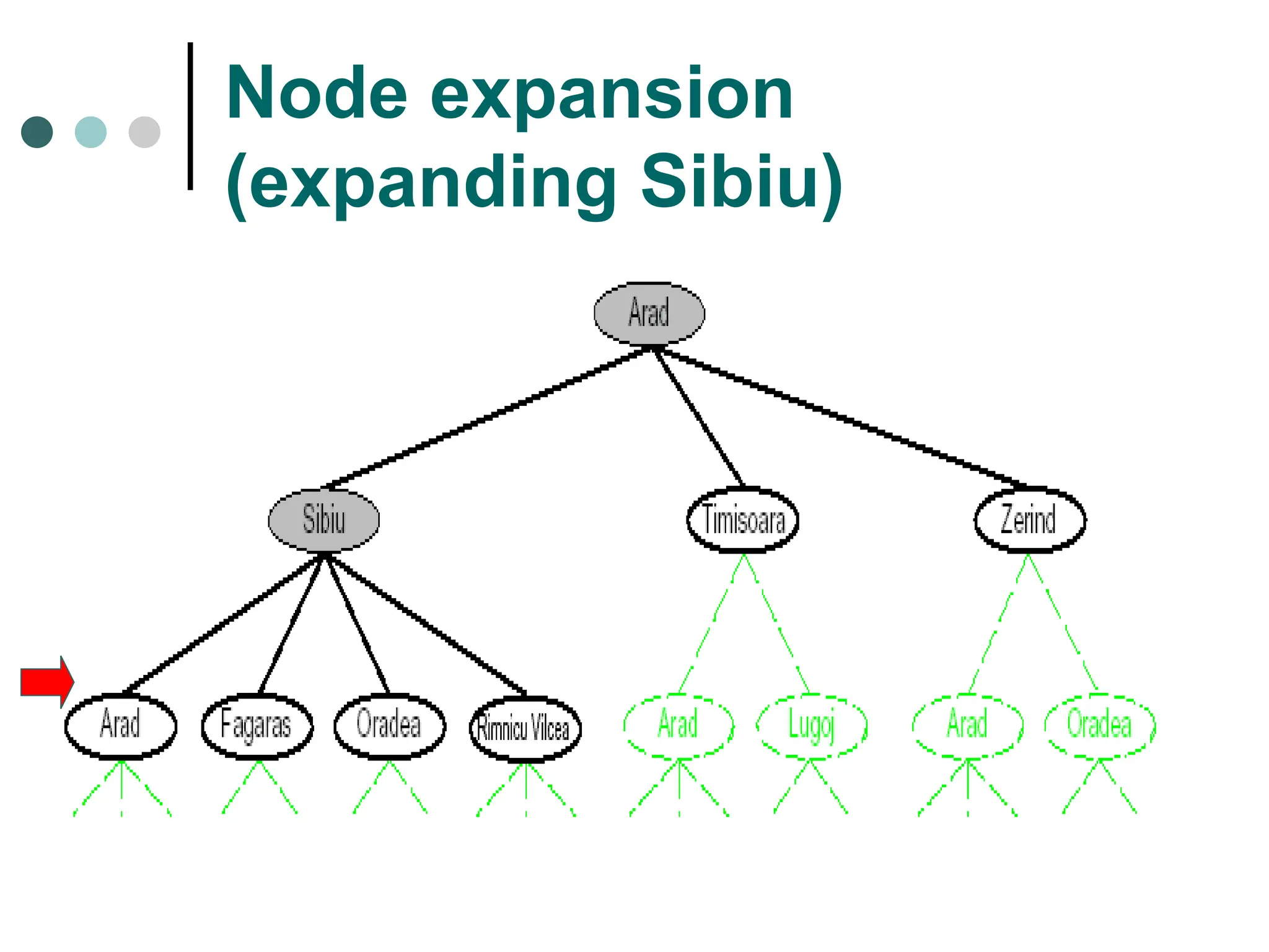
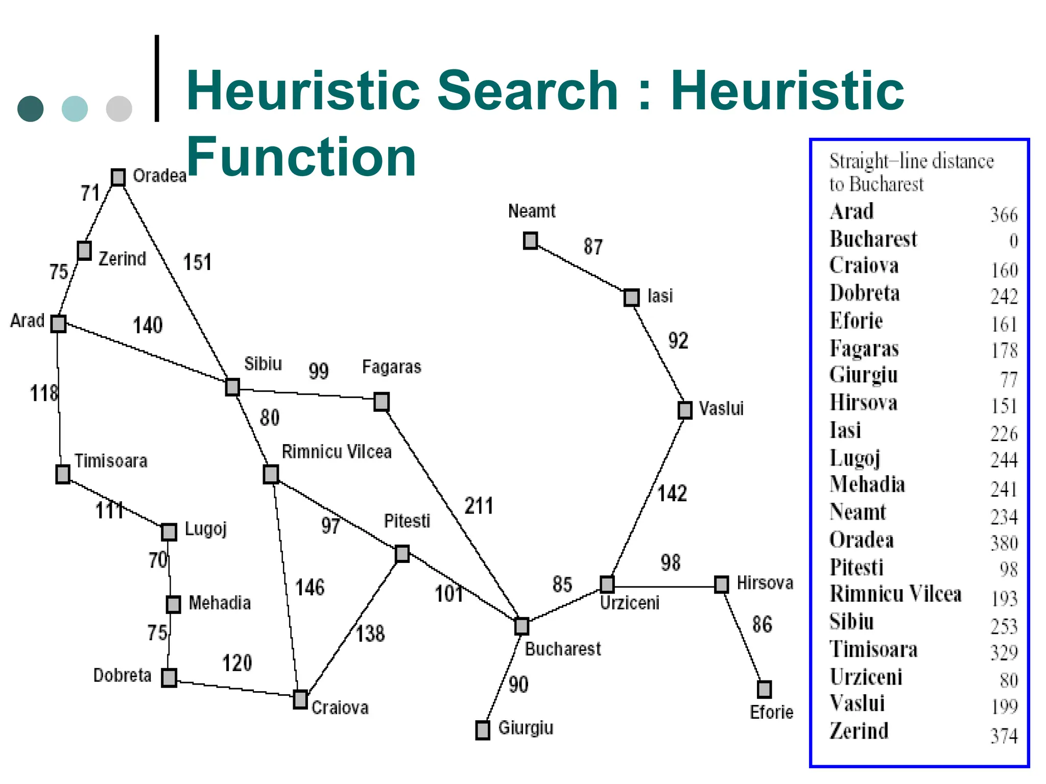
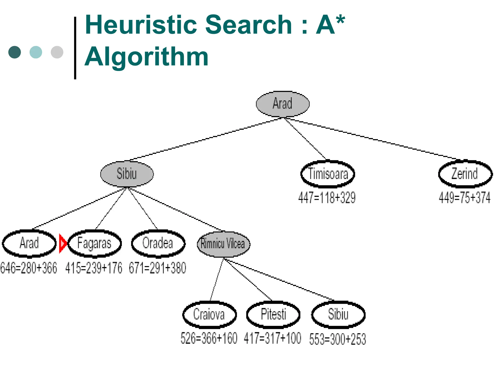
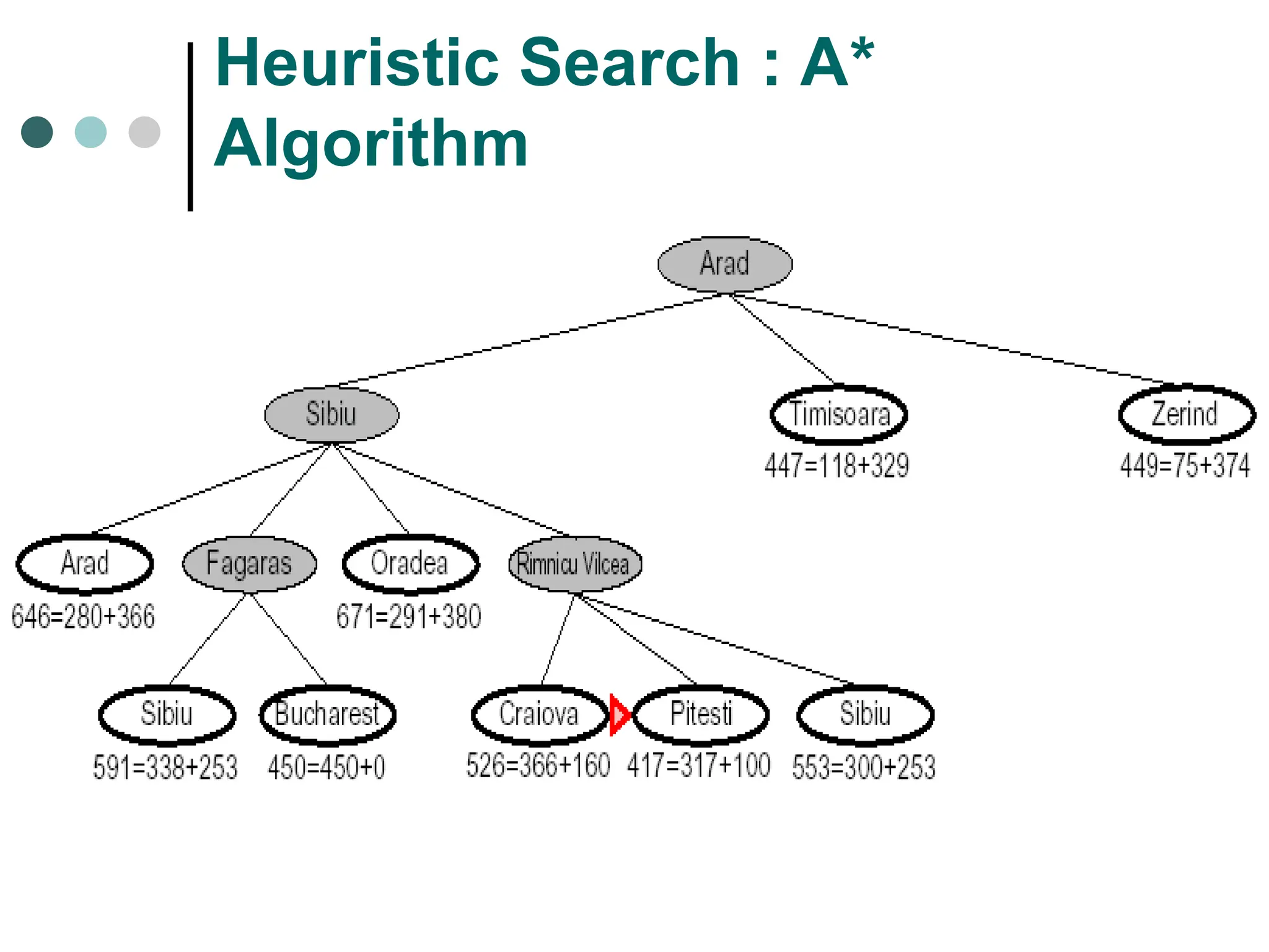
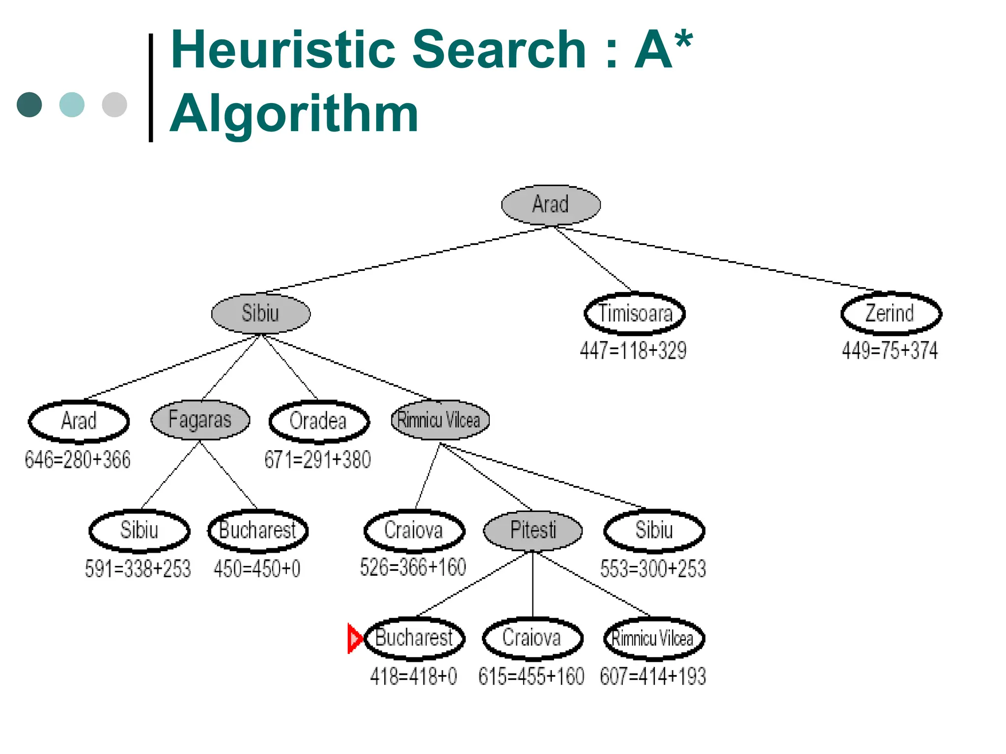
Search tree tree representation of search space, showing possible solutions from initial state.


![Coded Agents – with UiPath SDK + LangGraph [Virtual Hands-on Workshop]](https://cdn.slidesharecdn.com/ss_thumbnails/codedagentsdeck-251215155422-5497c599-thumbnail.jpg?width=640&height=640&fit=bounds)


