aaaaaaaaaaaaaaaaaaaaaaaaaaaaaaaaaaaaaaaaaaaaaaaaaaaaaaaaaaaaaaaaaaaaaaaaaaaaaaaaaa

1. Module-II

2. Module-II : Problem-solving
Solving Problems by Searching, Problem-Solving Agents,
Formulating Problems, Well-defined problems and solutions,
Measuring problem-solving performance, Toy problems,
Searching for Solutions, Search Strategies, Avoiding Repeated
States, Constraint Satisfaction Search, Informed Search
Methods, Best-First Search, Heuristic Functions, Memory
Bounded Search, Iterative Improvement Algorithms,
Applications in constraint satisfaction problems.

3. Problem Solving -Definition
• Problem solving is a process of generating solutions from
observed data.
• Problem is characterized by a set of goals, set of objects and
set of operations.
• The method of solving problem through AI involves the
process of
 Defining the search space.
 Deciding start and goal states
 Finding the path from start state to goal state through
search space.

4. Problem Solving
• Here search space or problem space is abstract space which
has all valid states that can be generated by the application of
any combination of operators or objects.
• A problem space can have one or more on solutions.
• Solution is combination of objects and operations that achieve
the goals.
• Search refers a search of solution in problem space.

5. Goal Based Agent or problem solving Agent
• Goal Based agents are usually called planning agents.
• Problem solving begins with the definitions of problems and
their solutions.
• We then describe several general purpose search algorithms
that can be used to solve these problems.
• We will see several uninformed search algorithms- algorithms
that are given no information about the problem other than its
definition.
• Informed search algorithms, on the other hand can do quite
well given some guidance on where to look for solutions.

6. Problem solving Agent
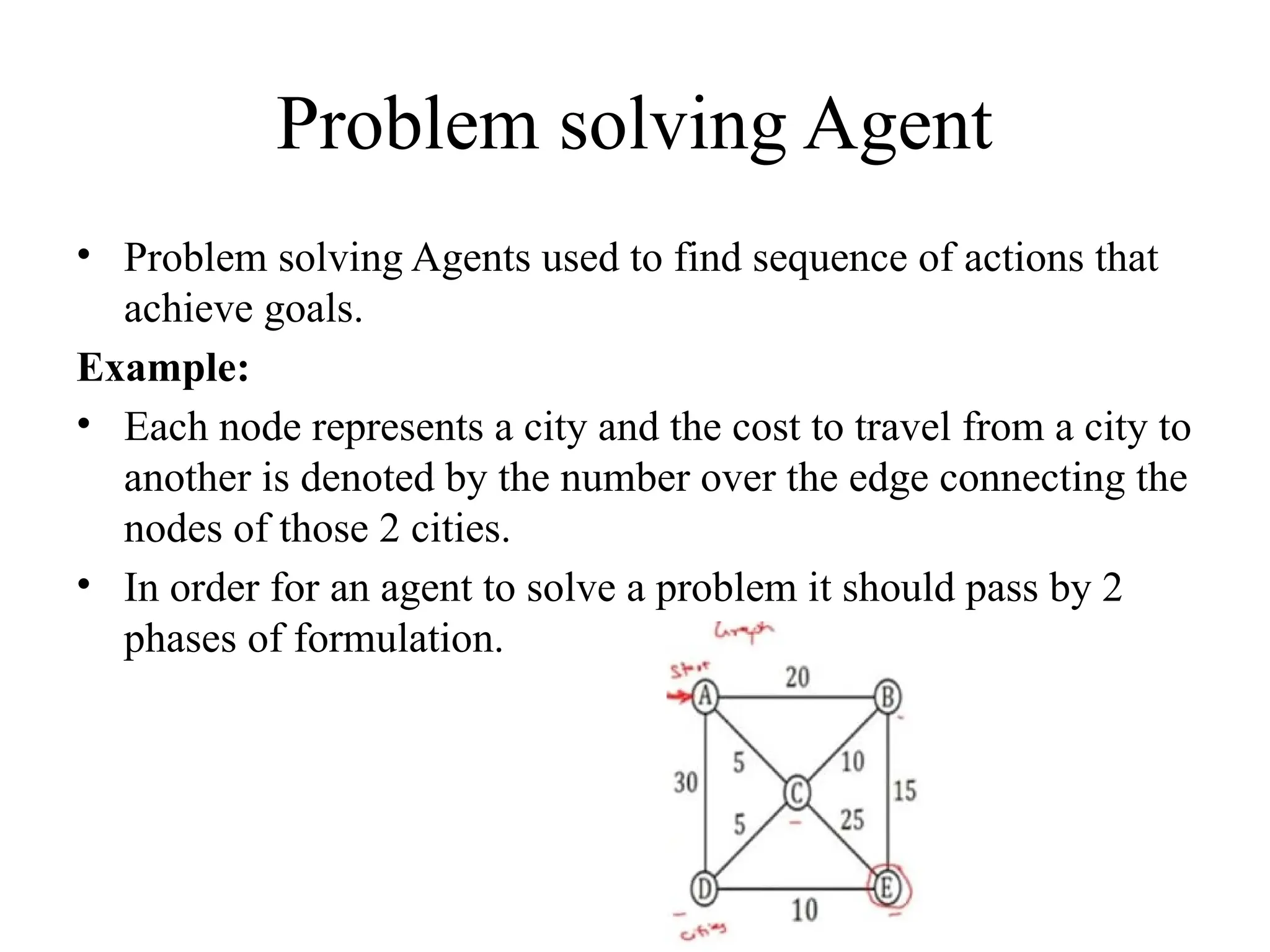
• Problem solving Agents used to find sequence of actions that
achieve goals.
Example:
• Each node represents a city and the cost to travel from a city to
another is denoted by the number over the edge connecting the
nodes of those 2 cities.
• In order for an agent to solve a problem it should pass by 2
phases of formulation.

7. Goal Formulation and Problem formulation
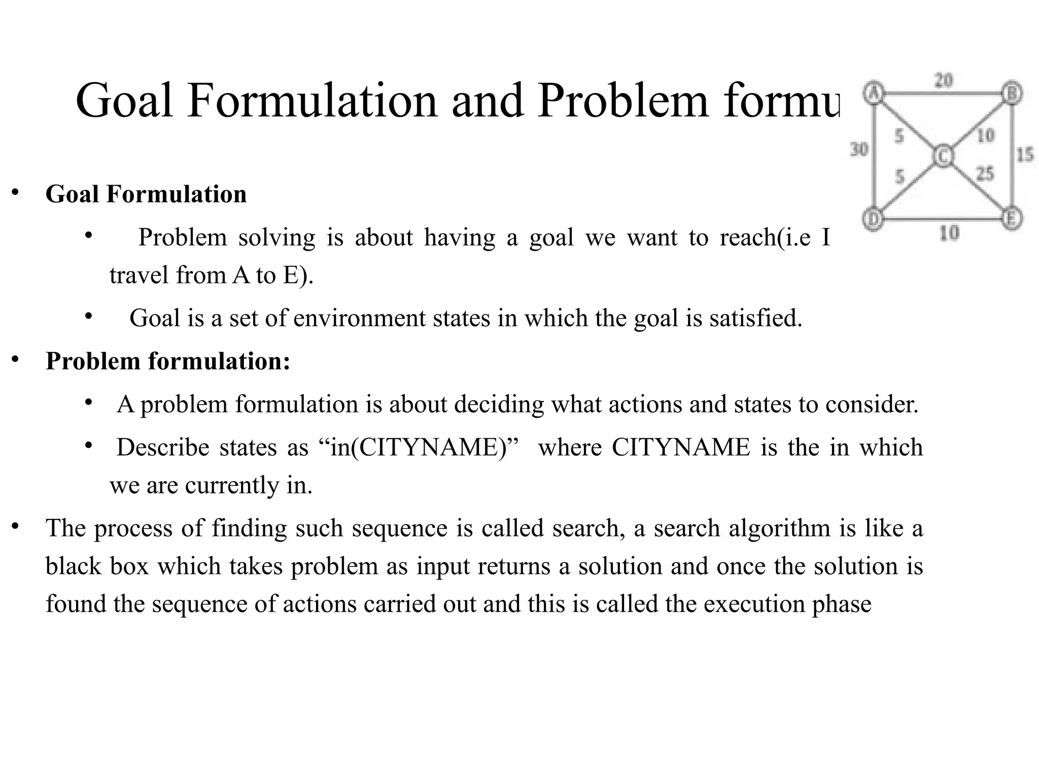
• Goal Formulation
• Problem solving is about having a goal we want to reach(i.e I want to
travel from A to E).
• Goal is a set of environment states in which the goal is satisfied.
• Problem formulation:
• A problem formulation is about deciding what actions and states to consider.
• Describe states as “in(CITYNAME)” where CITYNAME is the in which
we are currently in.
• The process of finding such sequence is called search, a search algorithm is like a
black box which takes problem as input returns a solution and once the solution is
found the sequence of actions carried out and this is called the execution phase

8. Formulating problems
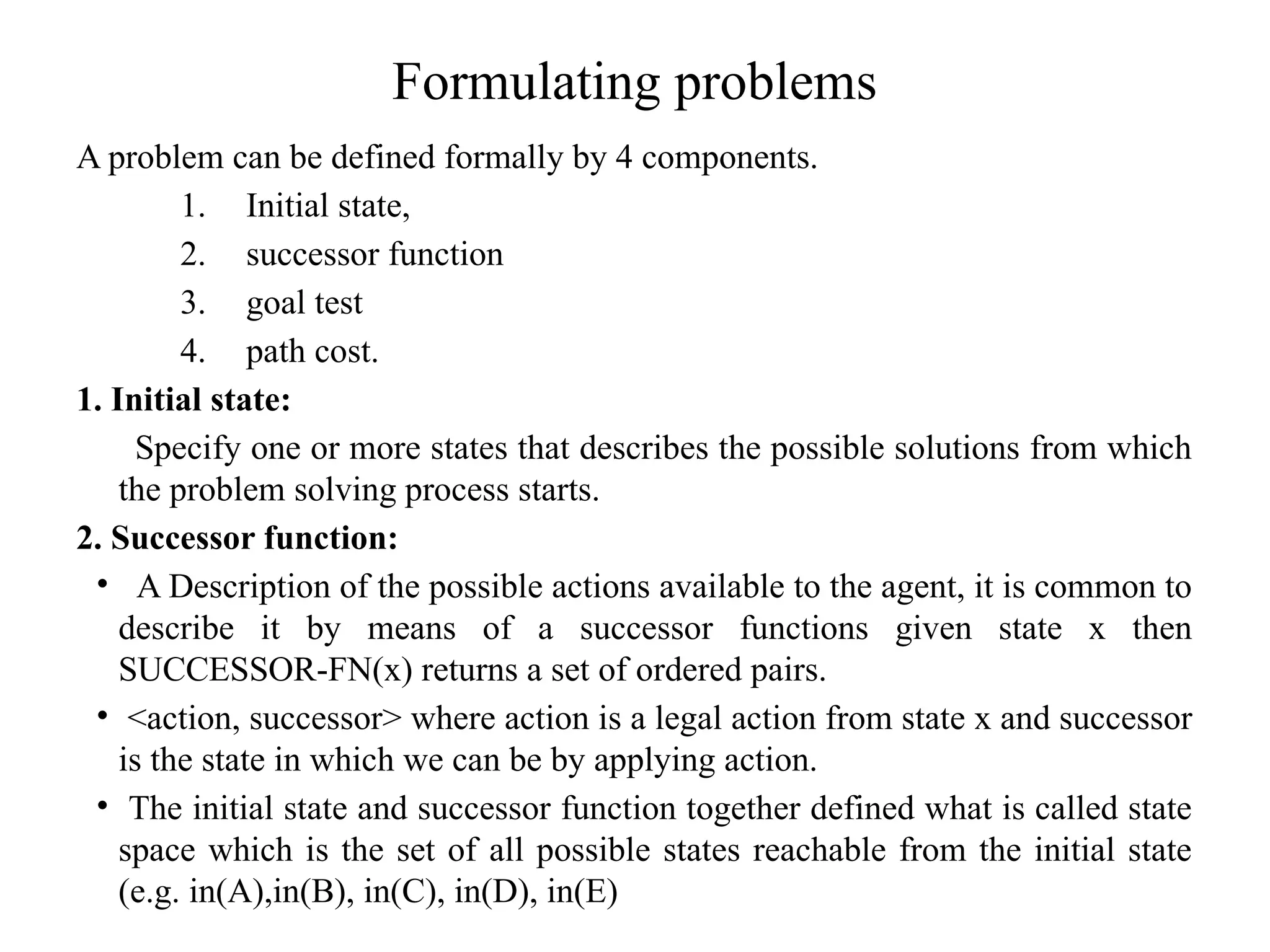
A problem can be defined formally by 4 components.
1. Initial state,
2. successor function
3. goal test
4. path cost.
1. Initial state:
Specify one or more states that describes the possible solutions from which
the problem solving process starts.
2. Successor function:
• A Description of the possible actions available to the agent, it is common to
describe it by means of a successor functions given state x then
SUCCESSOR-FN(x) returns a set of ordered pairs.
• <action, successor> where action is a legal action from state x and successor
is the state in which we can be by applying action.
• The initial state and successor function together defined what is called state
space which is the set of all possible states reachable from the initial state
(e.g. in(A),in(B), in(C), in(D), in(E)

9. Formulating problems
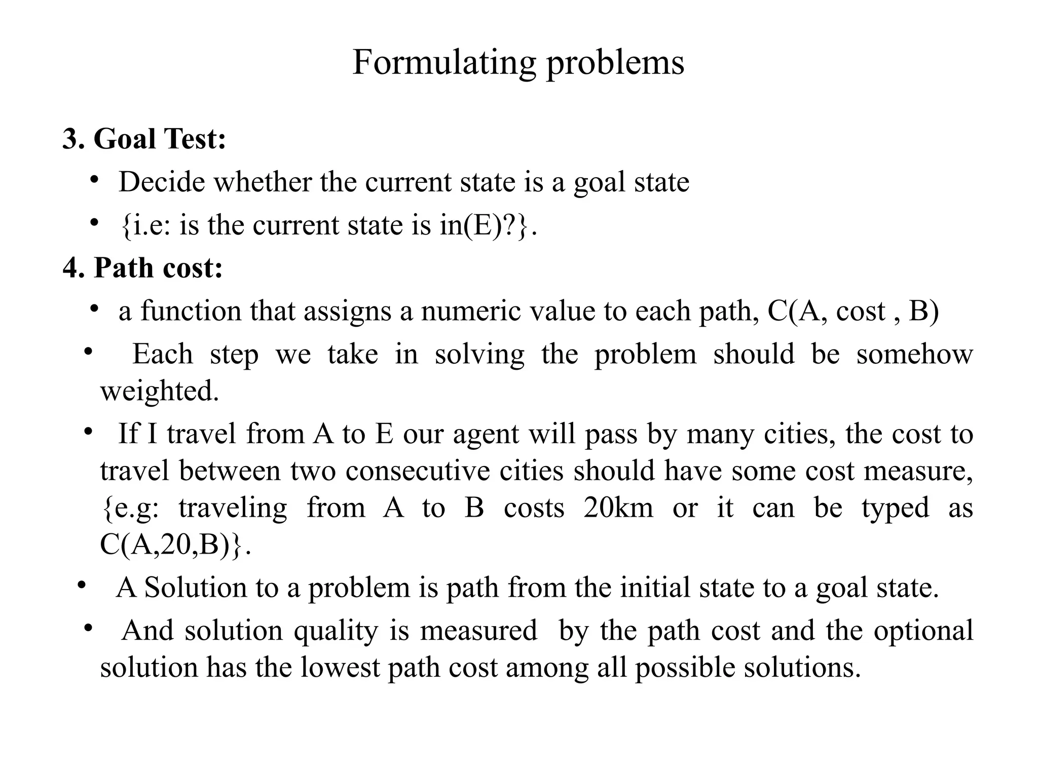
3. Goal Test:
• Decide whether the current state is a goal state
• {i.e: is the current state is in(E)?}.
4. Path cost:
• a function that assigns a numeric value to each path, C(A, cost , B)
• Each step we take in solving the problem should be somehow
weighted.
• If I travel from A to E our agent will pass by many cities, the cost to
travel between two consecutive cities should have some cost measure,
{e.g: traveling from A to B costs 20km or it can be typed as
C(A,20,B)}.
• A Solution to a problem is path from the initial state to a goal state.
• And solution quality is measured by the path cost and the optional
solution has the lowest path cost among all possible solutions.

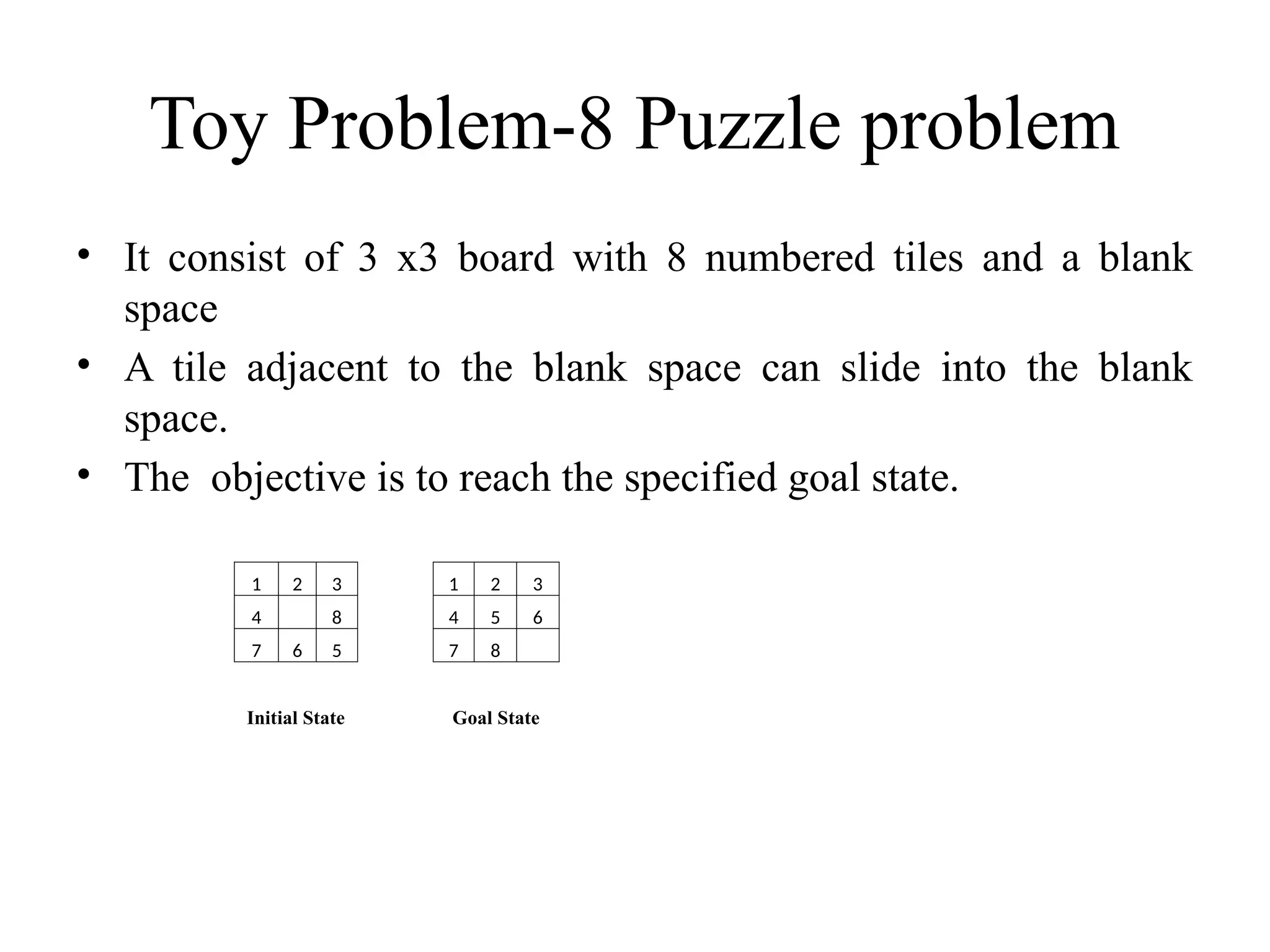
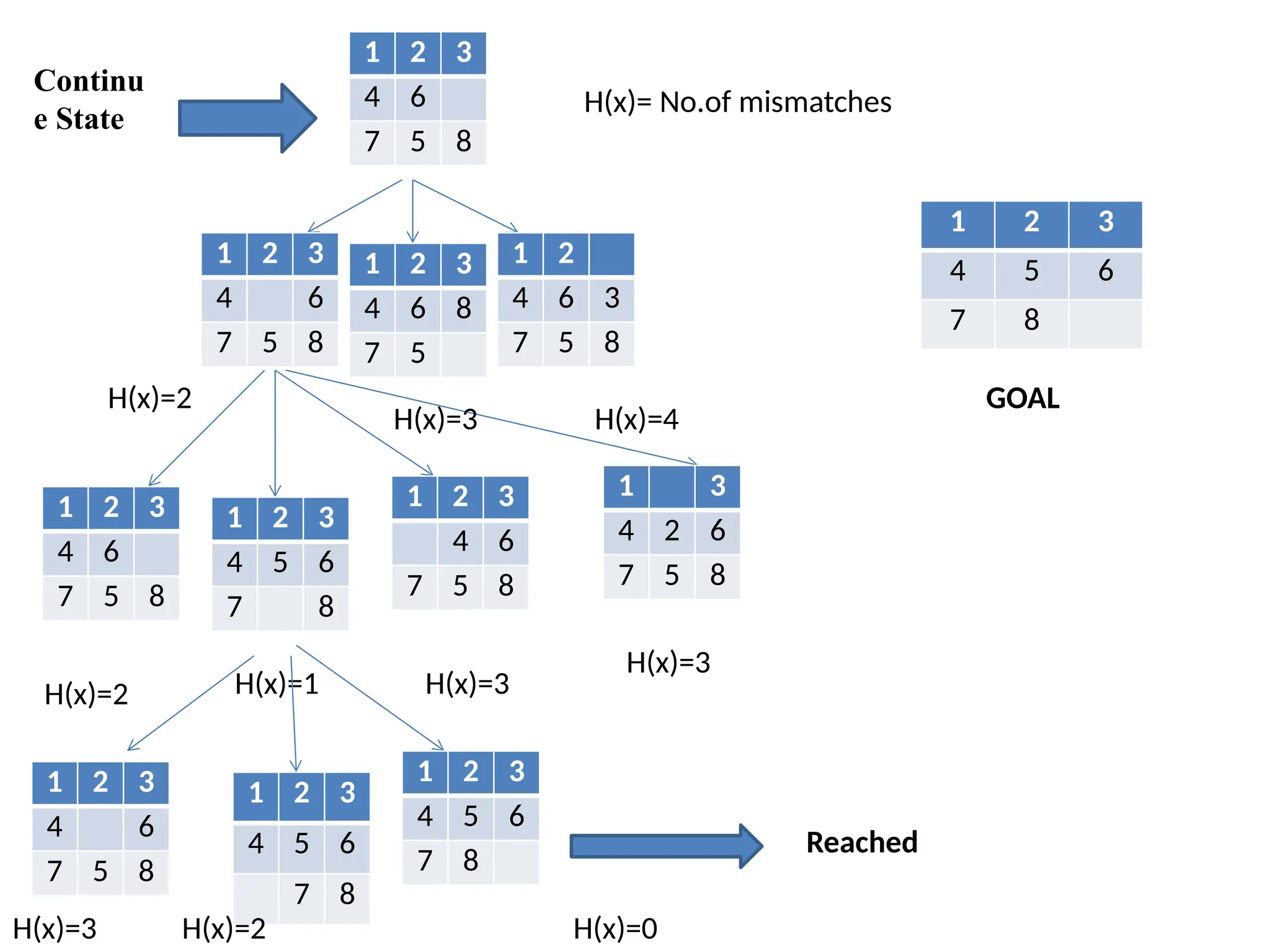
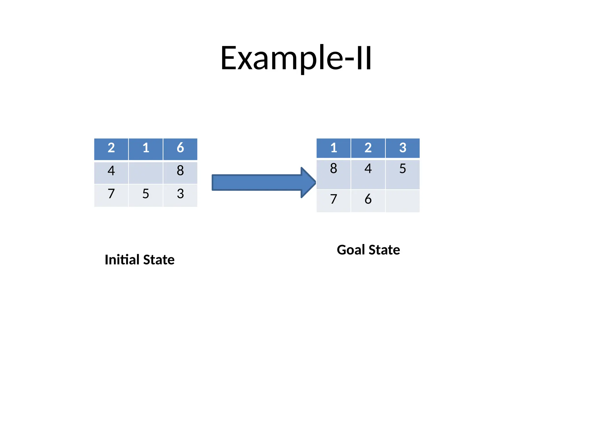
10. Toy Problem-8 Puzzle problem
• It consist of 3 x3 board with 8 numbered tiles and a blank
space
• A tile adjacent to the blank space can slide into the blank
space.
• The objective is to reach the specified goal state.
1 2 3 1 2 3
4 8 4 5 6
7 6 5 7 8
Initial State Goal State

11. Toy Problem-8 Puzzle problem
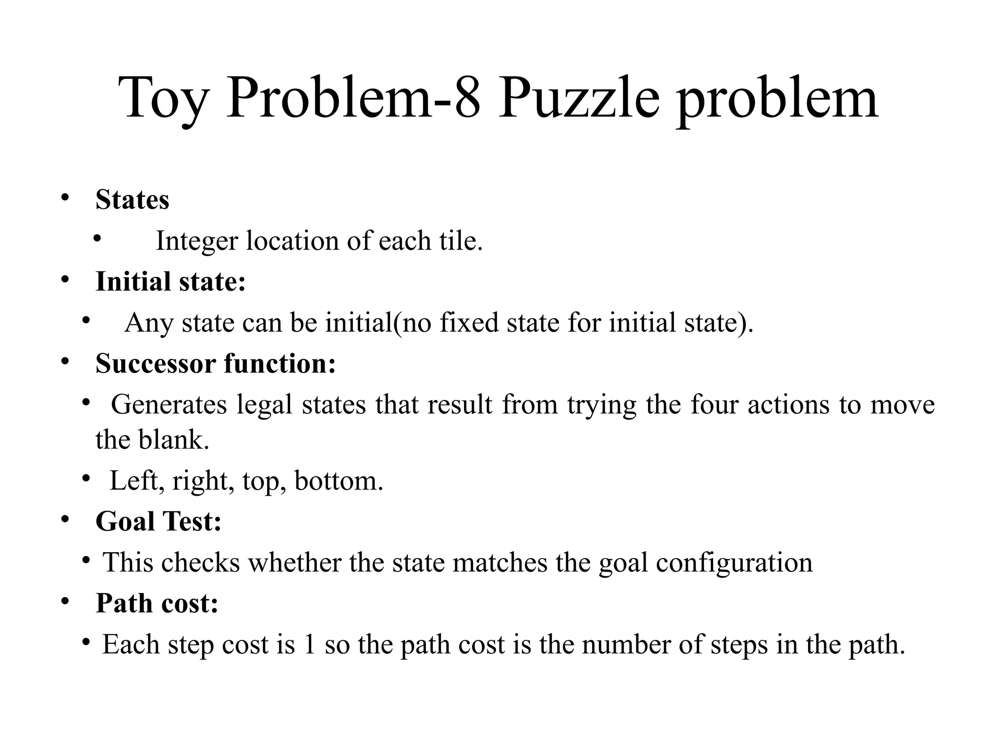
• States
• Integer location of each tile.
• Initial state:
• Any state can be initial(no fixed state for initial state).
• Successor function:
• Generates legal states that result from trying the four actions to move
the blank.
• Left, right, top, bottom.
• Goal Test:
• This checks whether the state matches the goal configuration
• Path cost:
• Each step cost is 1 so the path cost is the number of steps in the path.

12. 1 2 3
4 8
7 6 5
1 2 3
4 5 6
7 8
1 3
4 2 8
7 6 5
1 2 3
4 8
7 6 5
1 2 3
4 8
7 6 5
1 2 3
4 6 8
7 5
1 2 3
4 6 8
7 5
1 2 3
4 6 8
7 5
1 2 3
4 8
7 6 5
1 2 3
4 6
7 5 8
1 2 3
4 6 8
7 5
Initial
State
GOAL
H(x)=3 H(x)=4 H(x)=3
H(x)=4
H(x)=4
H(x)=3
H(x)=3
H(x)=3
H(x)=3
Heuristic function H(x)=
No.of mismatched places

13. 1 2 3
4 6
7 5 8
1 2
4 6 3
7 5 8
1 2 3
4 6 8
7 5
1 2 3
4 6
7 5 8
1 3
4 2 6
7 5 8
1 2 3
4 6
7 5 8
1 2 3
4 5 6
7 8
1 2 3
4 6
7 5 8
1 2 3
4 5 6
7 8
1 2 3
4 6
7 5 8
1 2 3
4 5 6
7 8
GOAL
Reached
Continu
e State
H(x)= No.of mismatches
H(x)=2
H(x)=3 H(x)=4
H(x)=2 H(x)=1 H(x)=3
H(x)=3
H(x)=3 H(x)=0
1 2 3
4 5 6
7 8
H(x)=2

14. Example-II
2 1 6
4 8
7 5 3
1 2 3
8 4 5
7 6
Initial State
Goal State

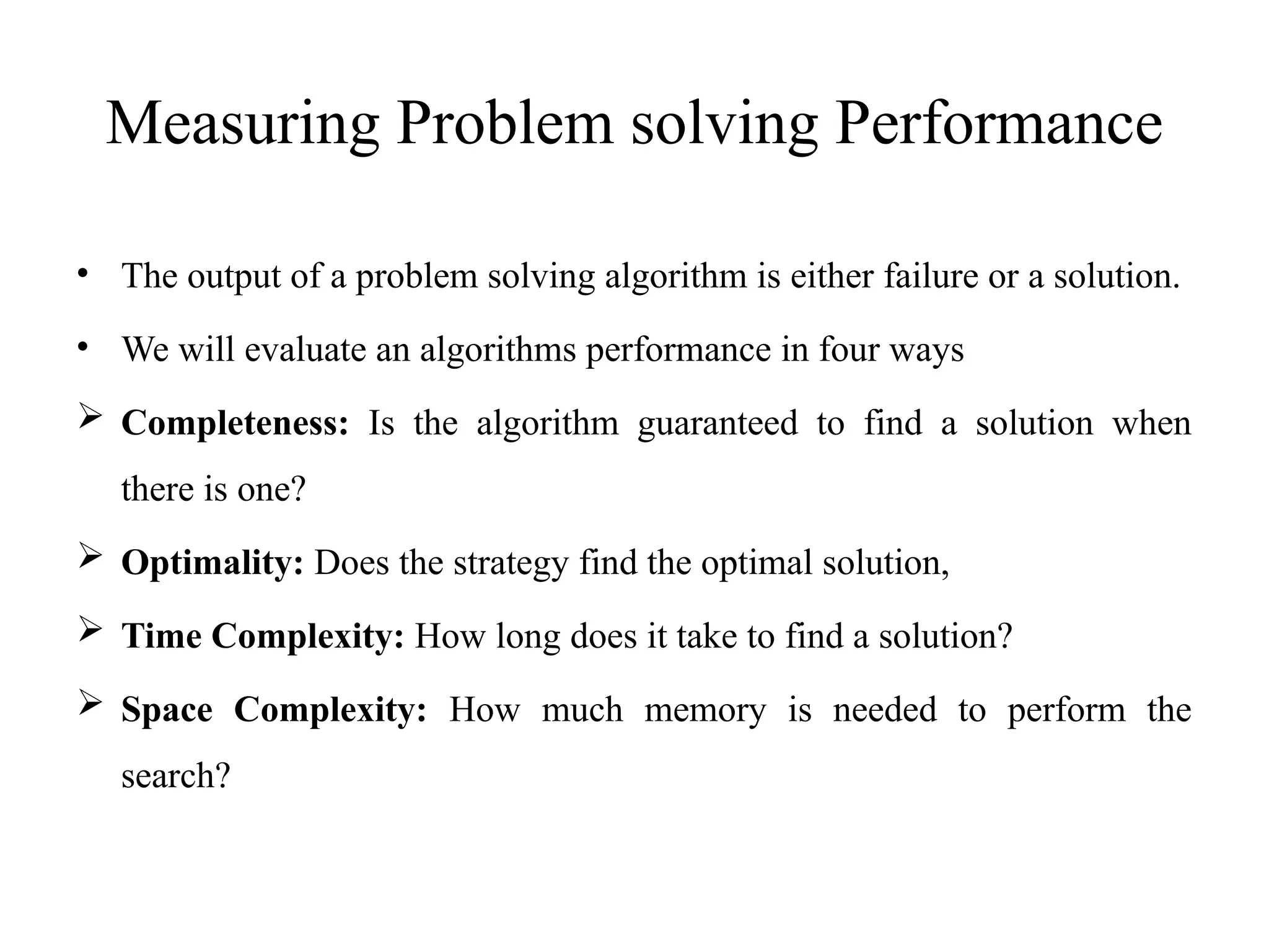
15. Measuring Problem solving Performance
• The output of a problem solving algorithm is either failure or a solution.
• We will evaluate an algorithms performance in four ways
 Completeness: Is the algorithm guaranteed to find a solution when
there is one?
 Optimality: Does the strategy find the optimal solution,
 Time Complexity: How long does it take to find a solution?
 Space Complexity: How much memory is needed to perform the
search?

16. Search Algorithm

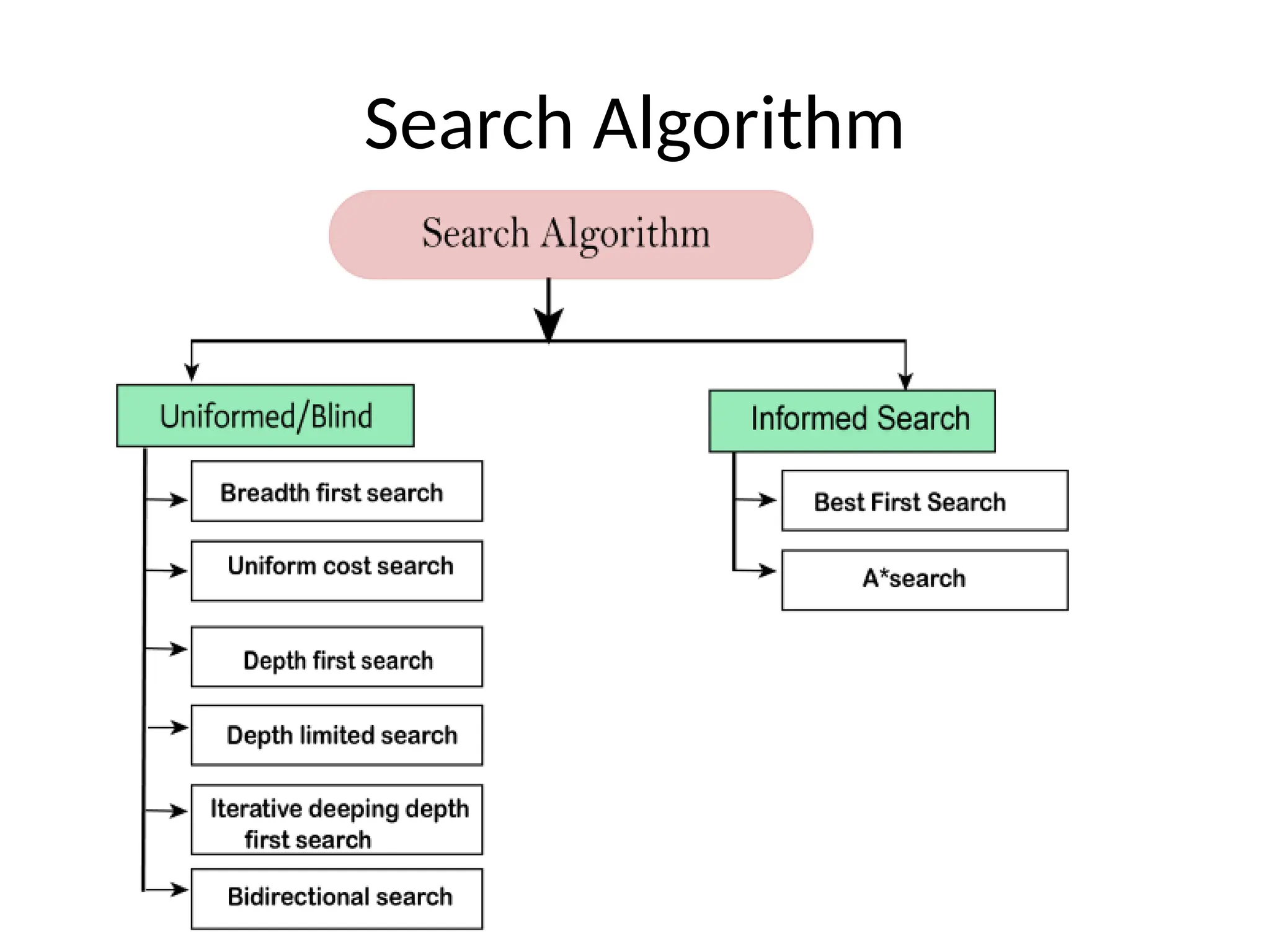
17. Uninformed Search algorithm
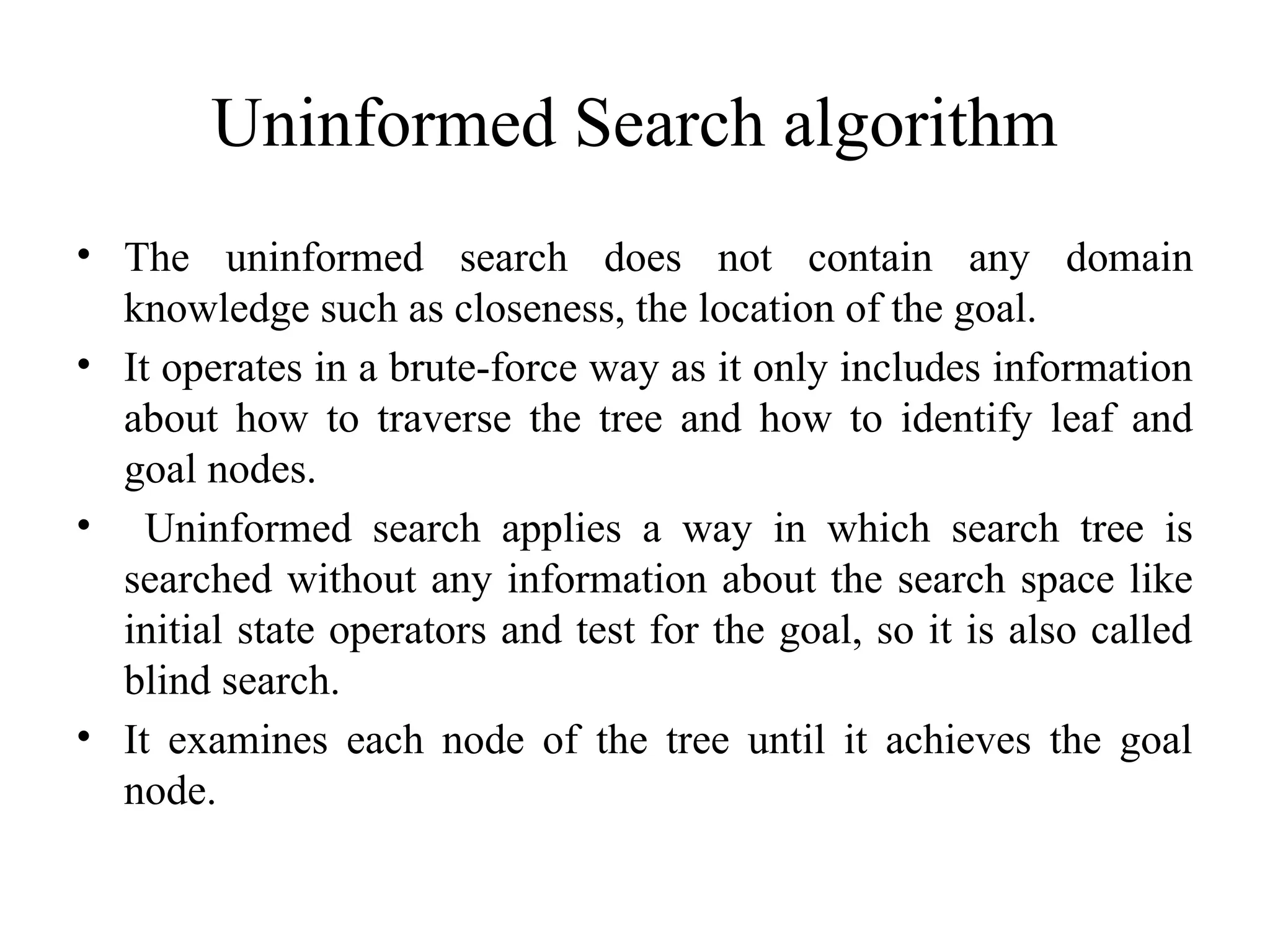
• The uninformed search does not contain any domain
knowledge such as closeness, the location of the goal.
• It operates in a brute-force way as it only includes information
about how to traverse the tree and how to identify leaf and
goal nodes.
• Uninformed search applies a way in which search tree is
searched without any information about the search space like
initial state operators and test for the goal, so it is also called
blind search.
• It examines each node of the tree until it achieves the goal
node.

18. Uninformed Search algorithm
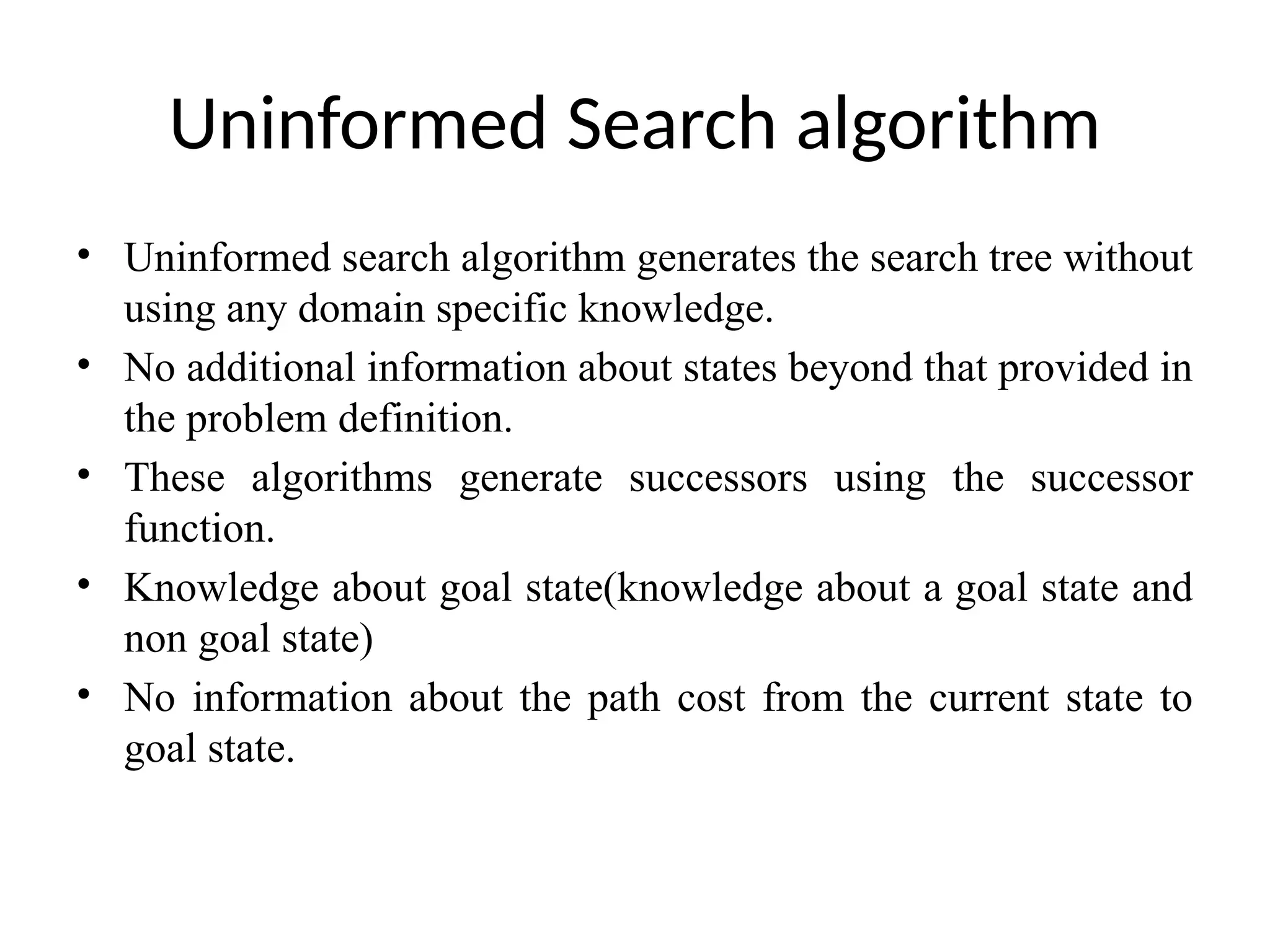
• Uninformed search algorithm generates the search tree without
using any domain specific knowledge.
• No additional information about states beyond that provided in
the problem definition.
• These algorithms generate successors using the successor
function.
• Knowledge about goal state(knowledge about a goal state and
non goal state)
• No information about the path cost from the current state to
goal state.

20. 1. Breadth-first Search
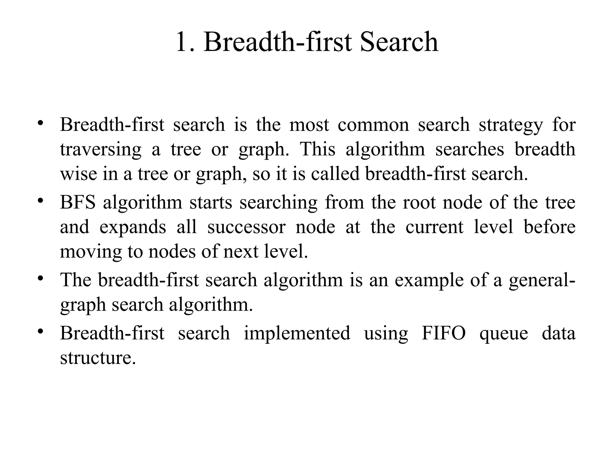
• Breadth-first search is the most common search strategy for
traversing a tree or graph. This algorithm searches breadth
wise in a tree or graph, so it is called breadth-first search.
• BFS algorithm starts searching from the root node of the tree
and expands all successor node at the current level before
moving to nodes of next level.
• The breadth-first search algorithm is an example of a general-
graph search algorithm.
• Breadth-first search implemented using FIFO queue data
structure.

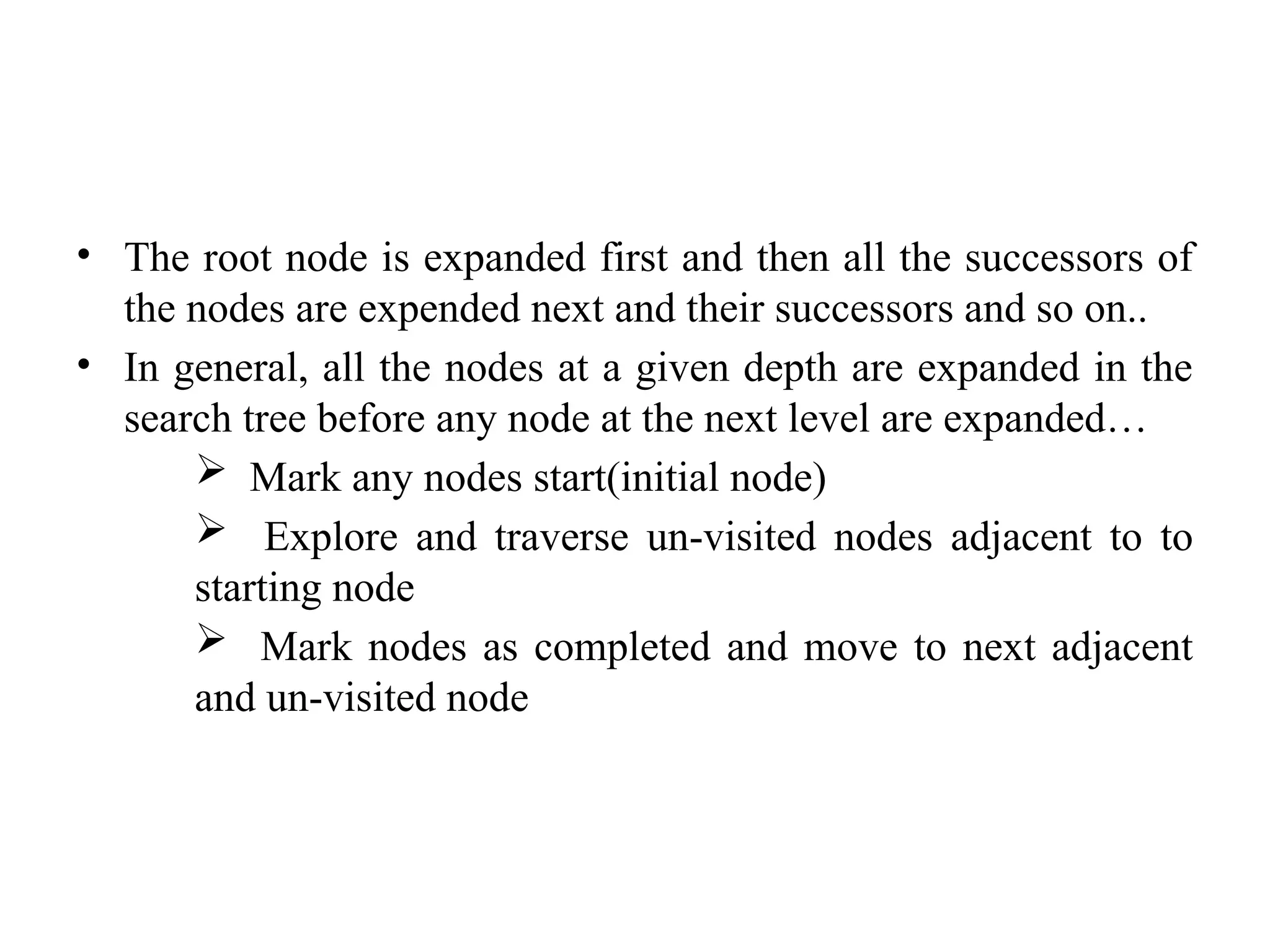
21. • The root node is expanded first and then all the successors of
the nodes are expended next and their successors and so on..
• In general, all the nodes at a given depth are expanded in the
search tree before any node at the next level are expanded…
 Mark any nodes start(initial node)
 Explore and traverse un-visited nodes adjacent to to
starting node
 Mark nodes as completed and move to next adjacent
and un-visited node

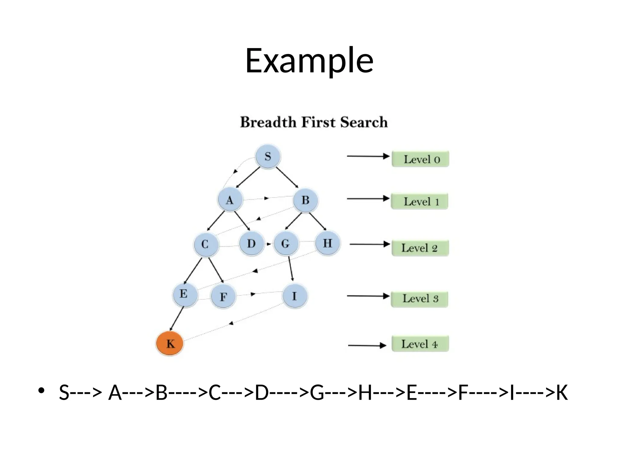
22. Example:
• In the below tree structure, we have shown the traversing of
the tree using BFS algorithm from the root node S to goal
node K. BFS search algorithm traverse in layers, so it will
follow the path which is shown by the dotted arrow, and the
traversed path will be:
• S---> A--->B---->C--->D---->G--->H--->E---->F---->I---->K

23. Example
• S---> A--->B---->C--->D---->G--->H--->E---->F---->I---->K

24. Advantages:
• BFS will provide a solution if any solution exists.
• If there are more than one solutions for a given problem, then
BFS will provide the minimal solution which requires the least
number of steps.
Disadvantages:
• It requires lots of memory since each level of the tree must be
saved into memory to expand the next level.
• BFS needs lots of time if the solution is far away from the root
node.

25. Performance analysis
Completeness: yes(if b is finite),the shallowest solution is returned
Time complexity: b+b2
+b3
+…..+bd
=O(bd
)
Time requirement is still a major factor
Space complexity: O(bd
)(keeps every node in memory.
Optimal: Yes if step costs are all identical or path cost is a non
decreasing function of the depth of the node.

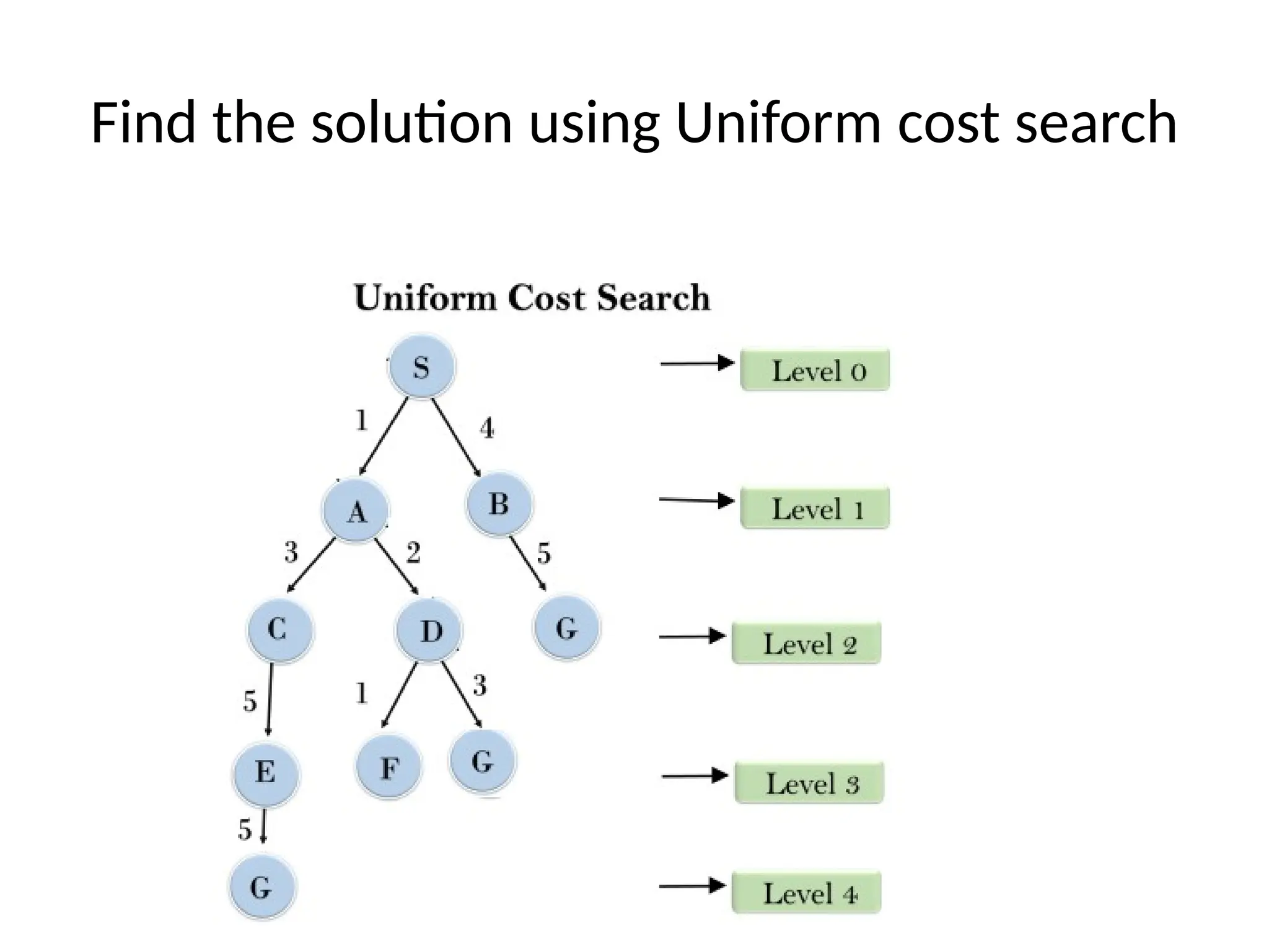
26. Uniform-cost search
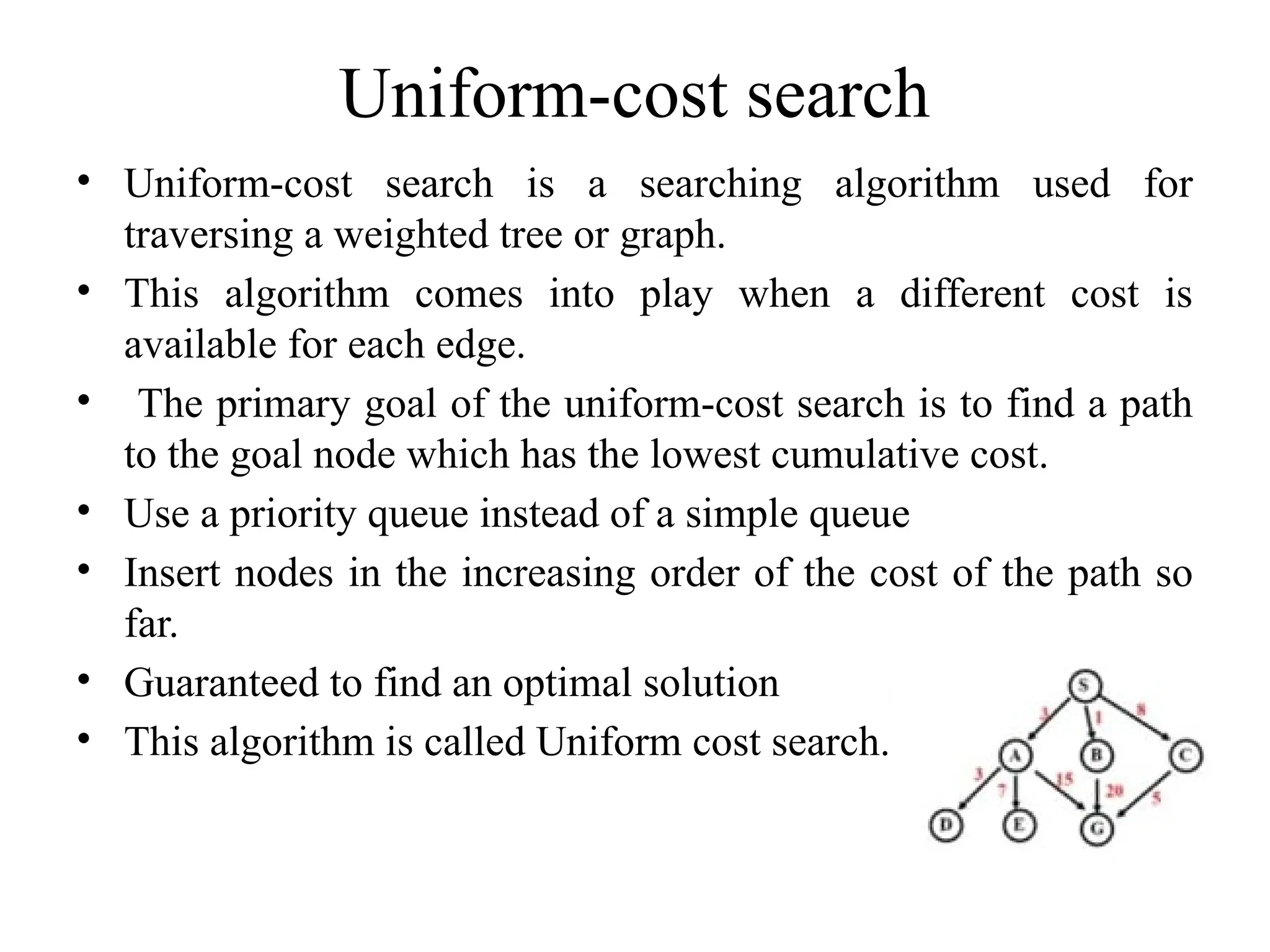
• Uniform-cost search is a searching algorithm used for
traversing a weighted tree or graph.
• This algorithm comes into play when a different cost is
available for each edge.
• The primary goal of the uniform-cost search is to find a path
to the goal node which has the lowest cumulative cost.
• Use a priority queue instead of a simple queue
• Insert nodes in the increasing order of the cost of the path so
far.
• Guaranteed to find an optimal solution
• This algorithm is called Uniform cost search.

27. • Uniform-cost search expands nodes according to their path
costs form the root node.
• It can be used to solve any graph/tree where the optimal cost is
in demand.
• A uniform-cost search algorithm is implemented by the
priority queue.
• It gives maximum priority to the lowest cumulative cost.
• Uniform cost search is equivalent to BFS algorithm if the path
cost of all edges is the same.

28. Uniform-cost search
• Enqueue nodes by path cost.
• That is let g(n)=cost of the path from the start node to the
current node n.
• Sort nodes by increasing value of g.

29. Example
A
15
G
S
B C
D E
3 8
1
5
20
7
3
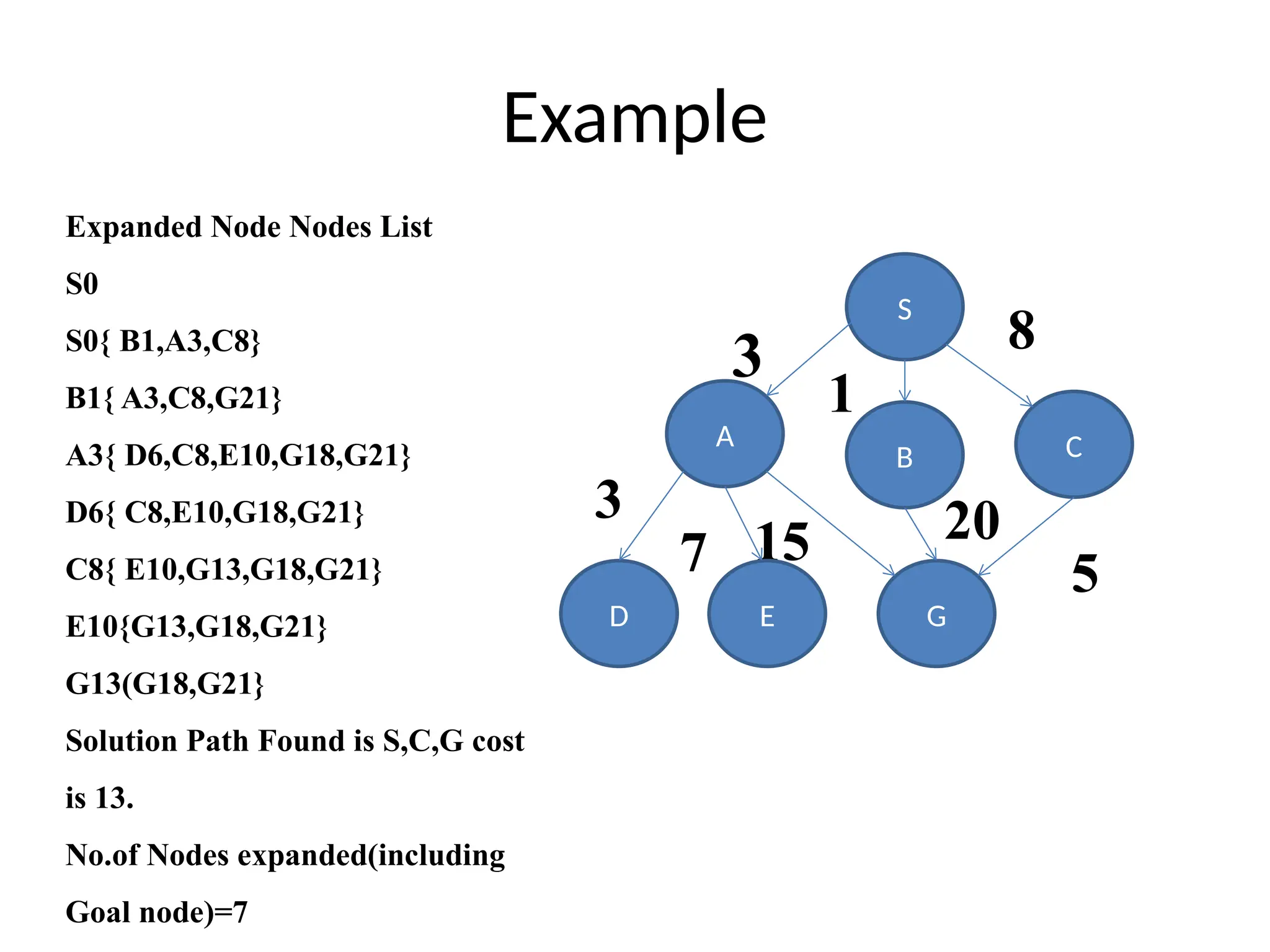
Expanded Node Nodes List
S0
S0{ B1,A3,C8}
B1{ A3,C8,G21}
A3{ D6,C8,E10,G18,G21}
D6{ C8,E10,G18,G21}
C8{ E10,G13,G18,G21}
E10{G13,G18,G21}
G13(G18,G21}
Solution Path Found is S,C,G cost
is 13.
No.of Nodes expanded(including
Goal node)=7

30. Advantages:
• Uniform cost search is optimal because at every state the path
with the least cost is chosen.
Disadvantages:
• It does not care about the number of steps involve in searching
and only concerned about path cost. Due to which this
algorithm may be stuck in an infinite loop.

31. Find the solution using Uniform cost search

32. 2. Depth-first Search
• Depth-first search is a recursive algorithm for traversing a tree
or graph data structure.
• It is called the depth-first search because it starts from the root
node and follows each path to its greatest depth node before
moving to the next path.
• DFS uses a stack data structure for its implementation.
• The process of the DFS algorithm is similar to the BFS
algorithm.

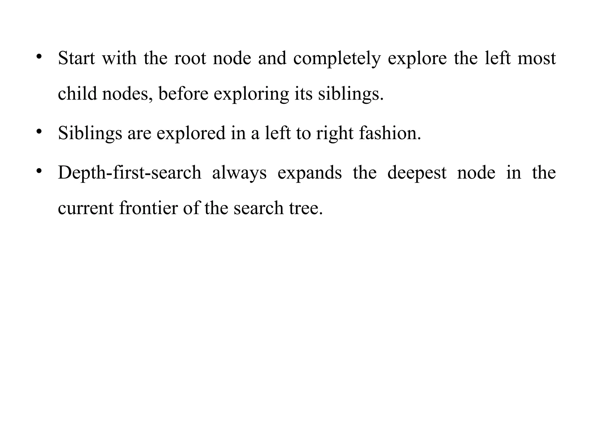
33. • Start with the root node and completely explore the left most
child nodes, before exploring its siblings.
• Siblings are explored in a left to right fashion.
• Depth-first-search always expands the deepest node in the
current frontier of the search tree.

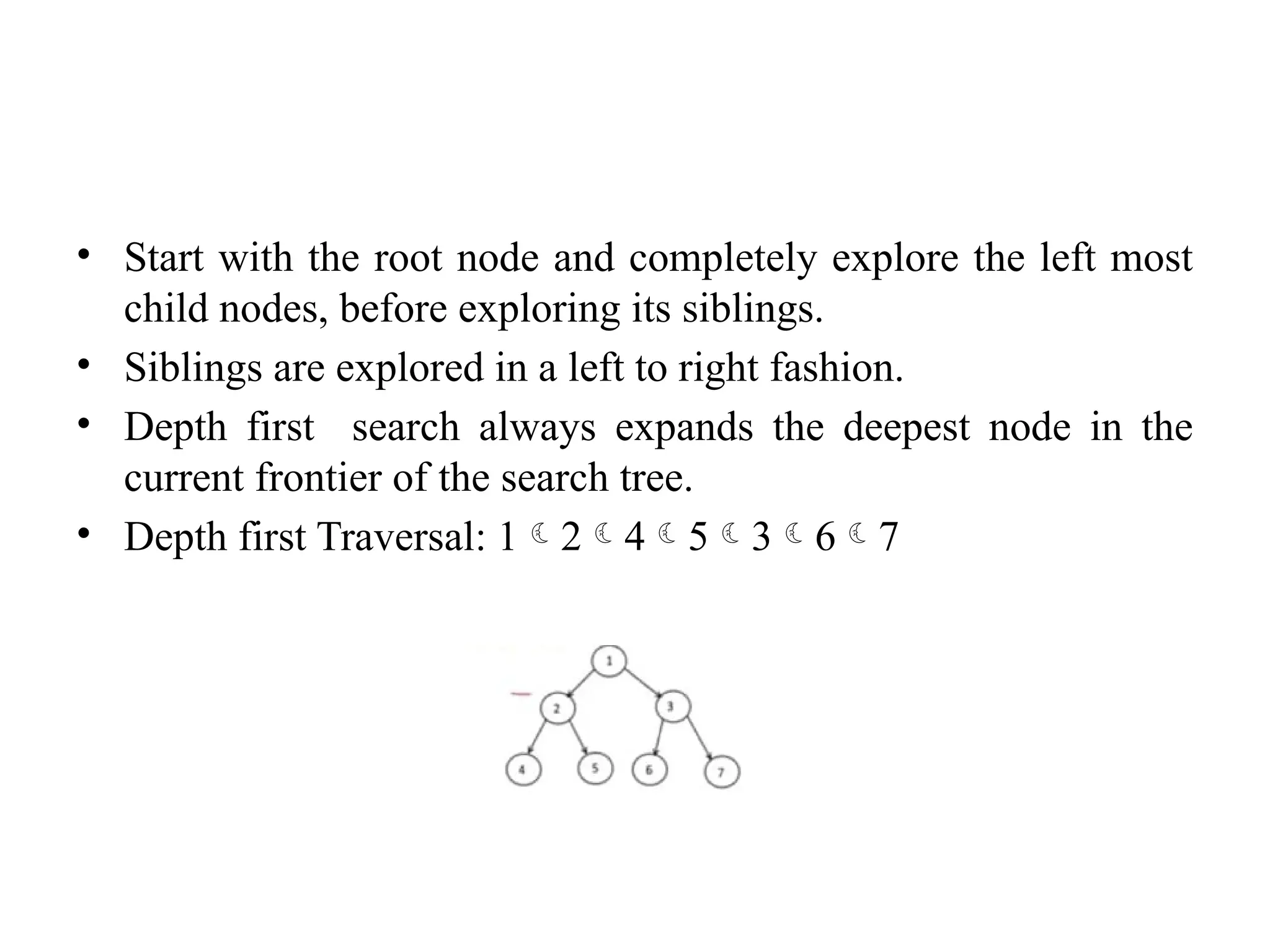
34. • Start with the root node and completely explore the left most
child nodes, before exploring its siblings.
• Siblings are explored in a left to right fashion.
• Depth first search always expands the deepest node in the
current frontier of the search tree.
• Depth first Traversal: 1245367

35. Example
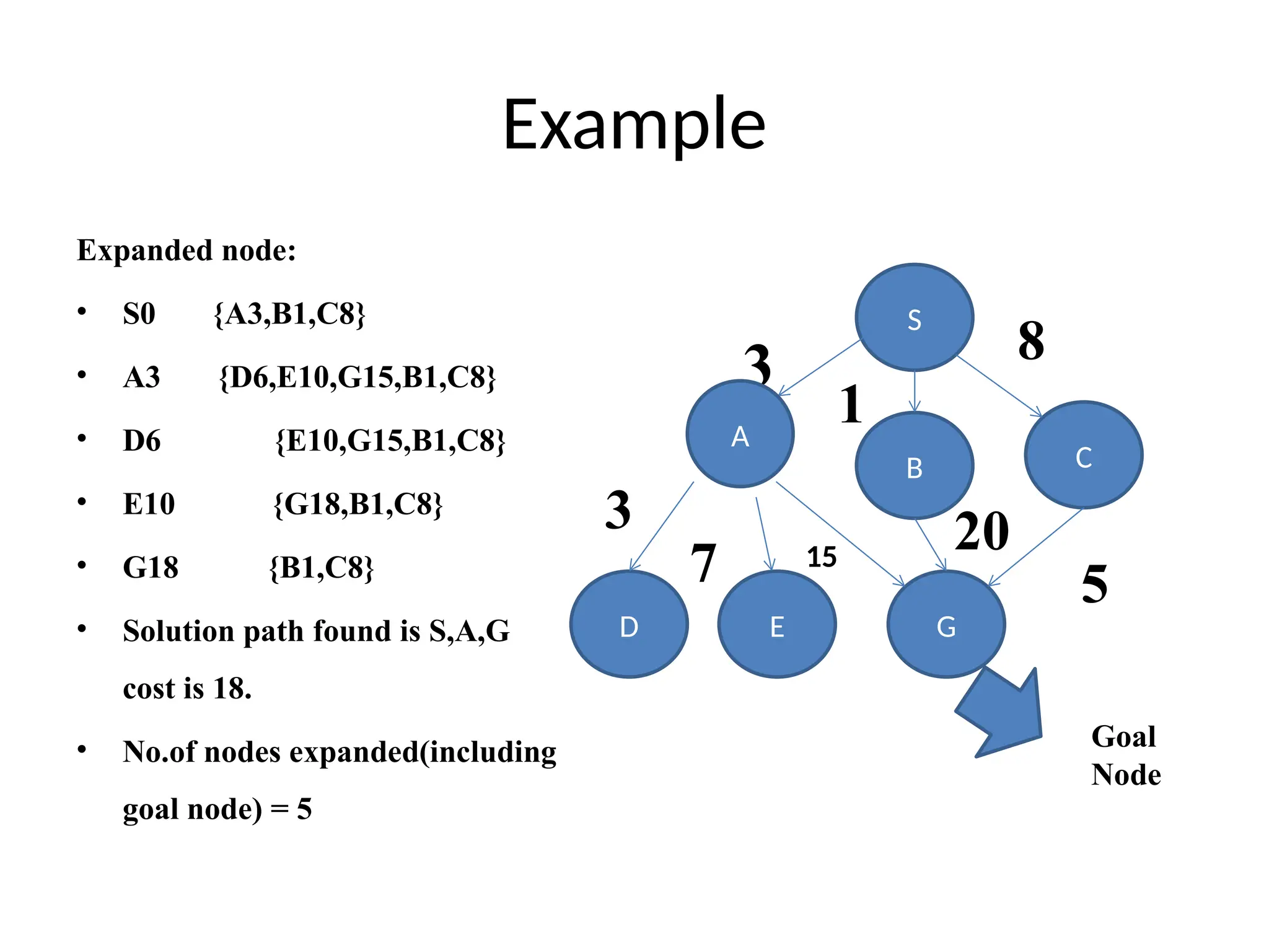
Expanded node:
• S0 {A3,B1,C8}
• A3 {D6,E10,G15,B1,C8}
• D6 {E10,G15,B1,C8}
• E10 {G18,B1,C8}
• G18 {B1,C8}
• Solution path found is S,A,G
cost is 18.
• No.of nodes expanded(including
goal node) = 5
G
S
B C
D E
3 8
1
5
20
7
3
A
15
Goal
Node

36. Advantage:
• DFS requires very less memory as it only needs to store a
stack of the nodes on the path from root node to the current
node.
• It takes less time to reach to the goal node than BFS algorithm
(if it traverses in the right path).
Disadvantage:
• There is the possibility that many states keep re-occurring, and
there is no guarantee of finding the optimal solution.
• DFS algorithm goes for deep down searching and sometime it
may go to the infinite loop.

37. Performance analysis
Completeness: yes
Time complexity: O(bm
)
Space complexity: O(bm
)(keeps every node in memory.
Optimal: No

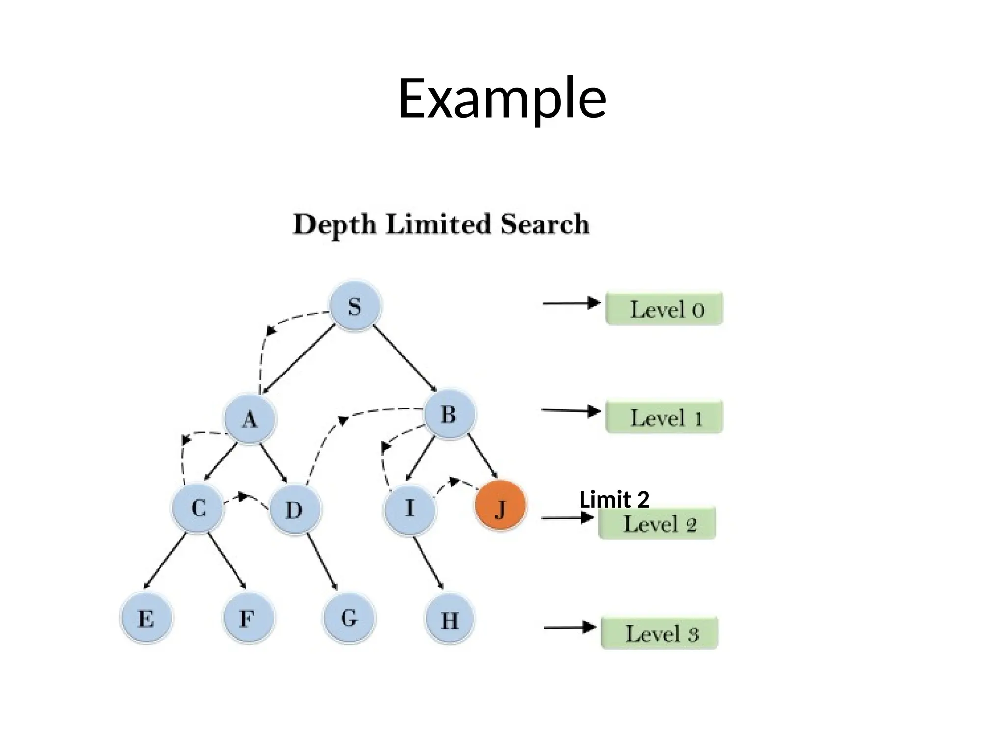
38. Depth-Limited Search Algorithm
• A depth-limited search algorithm is similar to depth-first
search with a predetermined limit.
• Depth-limited search can solve the drawback of the infinite
path in the Depth-first search.
• In this algorithm, the node at the depth limit will treat as it has
no successor nodes further.
Depth-limited search can be terminated with two Conditions
of failure:
• Standard failure value: It indicates that problem does not
have any solution.
• Cutoff failure value: It defines no solution for the problem
within a given depth limit.

39. Advantages:
• Depth-limited search is Memory efficient.
Disadvantages:
• Depth-limited search also has a disadvantage of
incompleteness.
• It may not be optimal if the problem has more than one
solution.

40. Example
Limit 2

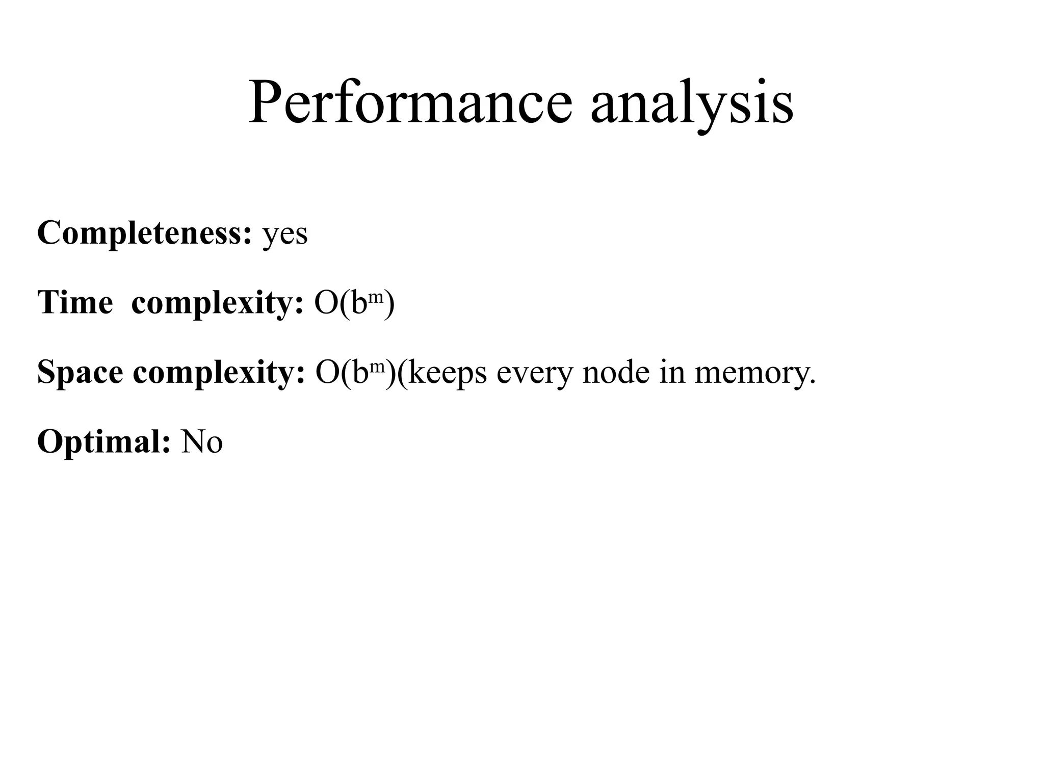
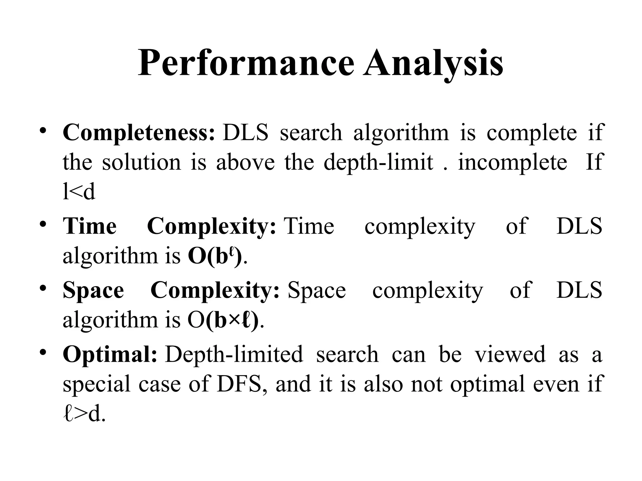
41. Performance Analysis
• Completeness: DLS search algorithm is complete if
the solution is above the depth-limit . incomplete If
l<d
• Time Complexity: Time complexity of DLS
algorithm is O(bℓ
).
• Space Complexity: Space complexity of DLS
algorithm is O(b×ℓ).
• Optimal: Depth-limited search can be viewed as a
special case of DFS, and it is also not optimal even if
ℓ>d.

42. Iterative deepening depth-first Search
• The iterative deepening algorithm is a combination of DFS and
BFS algorithms.
• This search algorithm finds out the best depth limit and does it
by gradually increasing the limit until a goal is found.
• This algorithm performs depth-first search up to a certain
"depth limit", and it keeps increasing the depth limit after each
iteration until the goal node is found.
• This Search algorithm combines the benefits of Breadth-first
search's fast search and depth-first search's memory efficiency.
• The iterative search algorithm is useful uninformed search
when search space is large, and depth of goal node is unknown.

43. Advantages:
• It combines the benefits of BFS and DFS search algorithm in
terms of fast search and memory efficiency.
Disadvantages:
• The main drawback of IDDFS is that it repeats all the work of
the previous phase.

44. Example

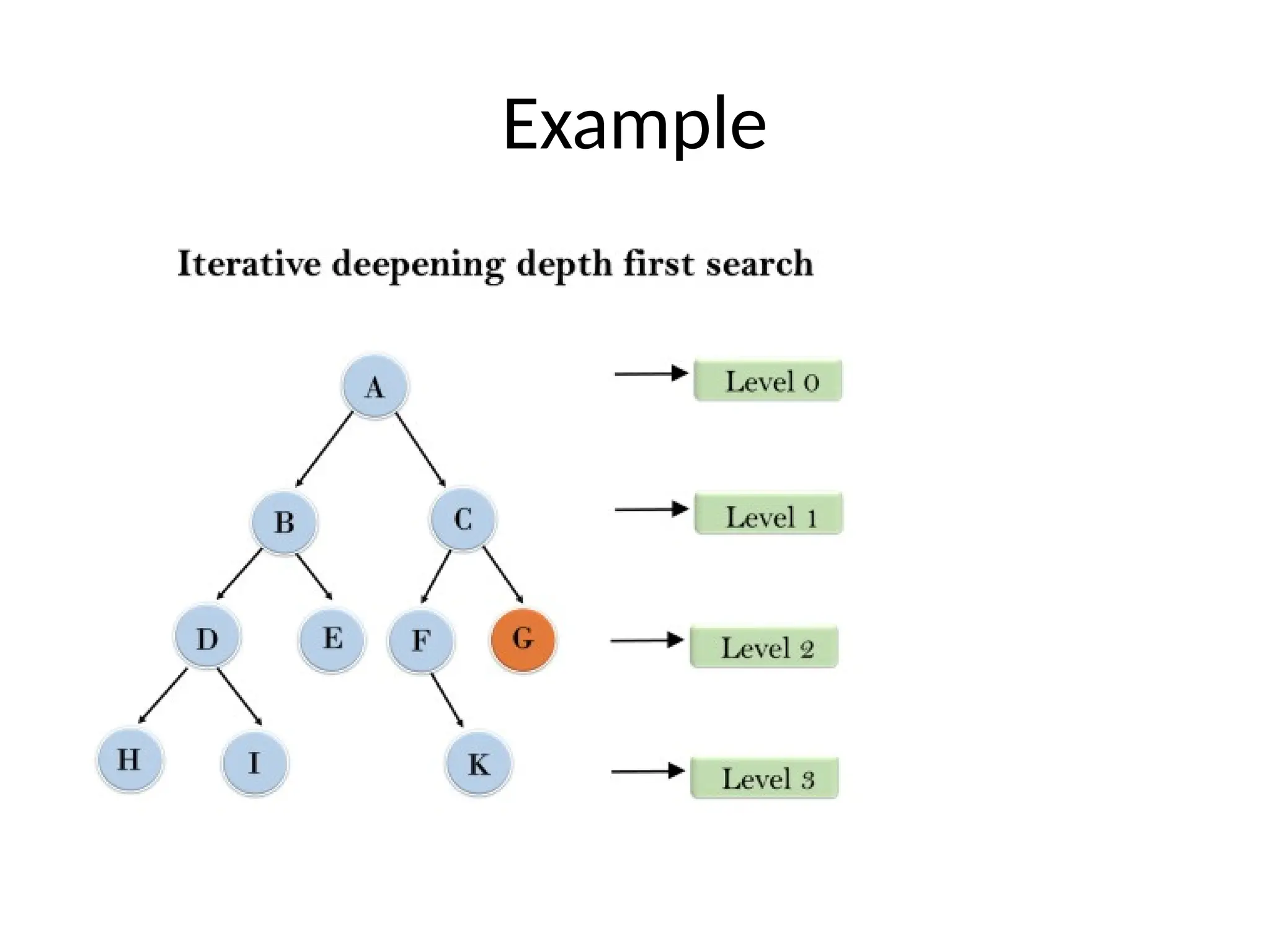
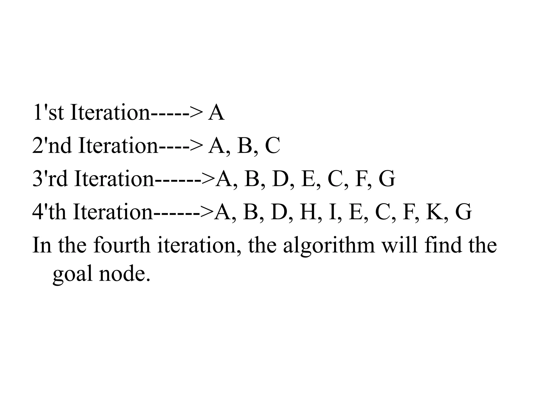
45. 1'st Iteration-----> A
2'nd Iteration----> A, B, C
3'rd Iteration------>A, B, D, E, C, F, G
4'th Iteration------>A, B, D, H, I, E, C, F, K, G
In the fourth iteration, the algorithm will find the
goal node.

46. Analysis
Completeness:
This algorithm is complete is if the branching factor is finite.
Time Complexity:
Let's suppose b is the branching factor and depth is d then
the worst-case time complexity is O(bd
).
Space Complexity:
The space complexity of IDDFS will be O(bd).
Optimal:
IDDFS algorithm is optimal if path cost is a non-
decreasing function of the depth of the node.

47. Informed Search Algorithms
Informed search algorithm contains an array of knowledge such
as
 how far we are from the goal
 path cost
 how to reach to goal node, etc.
This knowledge help agents to explore less to the search space
and find more efficiently the goal node.

48. • The informed search algorithm is more useful for large search space. Informed search
algorithm uses the idea of heuristic, so it is also called Heuristic search.
Heuristics function:
• Heuristic is a function which is used in Informed Search, and it finds the most
promising path.
• It takes the current state of the agent as its input and produces the estimation of
how close agent is from the goal.
• The heuristic method, however, might not always give the best solution, but it
guaranteed to find a good solution in reasonable time. Heuristic function
estimates how close a state is to the goal.
• It is represented by h(n), and it calculates the cost of an optimal path between
the pair of states.
• The value of the heuristic function is always positive.

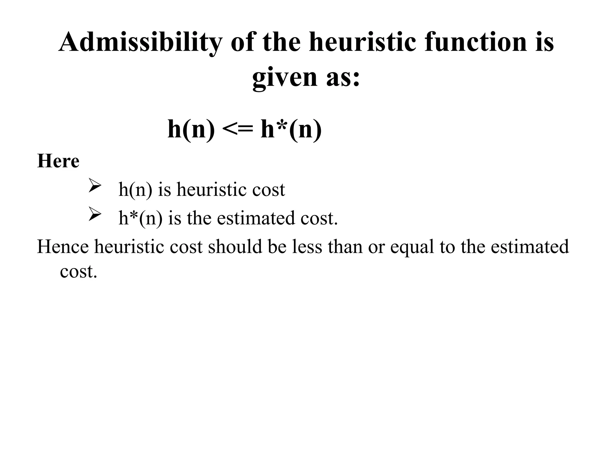
49. Admissibility of the heuristic function is
given as:
h(n) <= h*(n)
Here
 h(n) is heuristic cost
 h*(n) is the estimated cost.
Hence heuristic cost should be less than or equal to the estimated
cost.

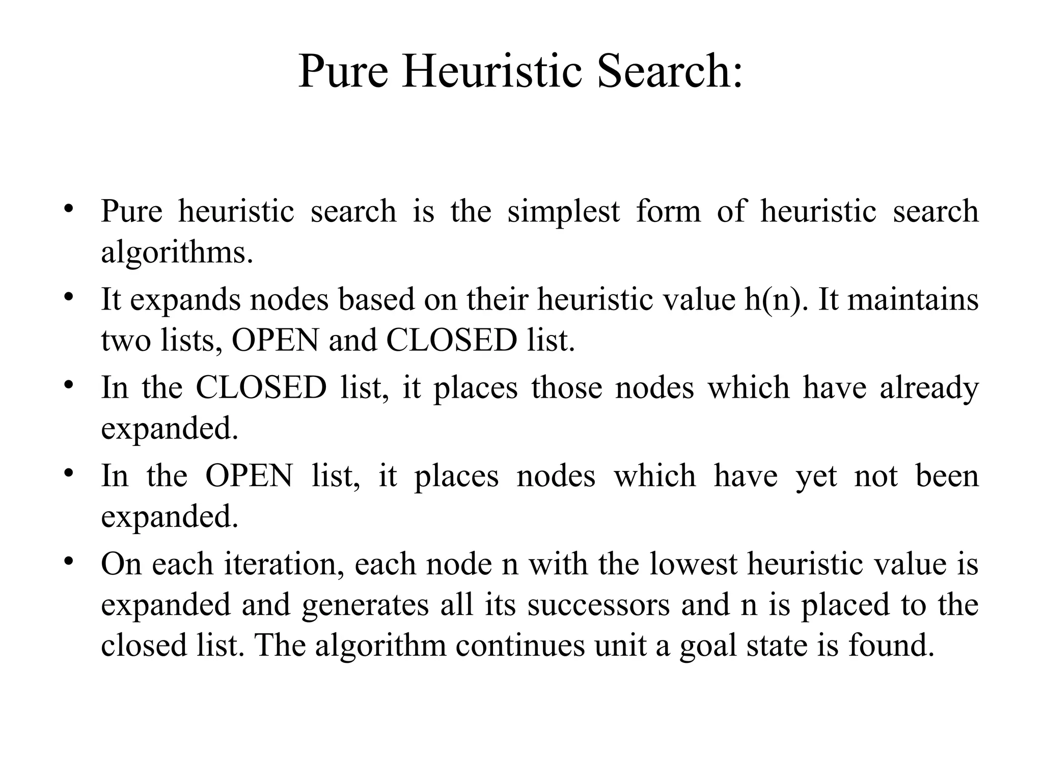
50. Pure Heuristic Search:
• Pure heuristic search is the simplest form of heuristic search
algorithms.
• It expands nodes based on their heuristic value h(n). It maintains
two lists, OPEN and CLOSED list.
• In the CLOSED list, it places those nodes which have already
expanded.
• In the OPEN list, it places nodes which have yet not been
expanded.
• On each iteration, each node n with the lowest heuristic value is
expanded and generates all its successors and n is placed to the
closed list. The algorithm continues unit a goal state is found.

51. In the informed search we will discuss two main algorithms
which are given below:
• Best First Search Algorithm(Greedy search)
• A* Search Algorithm

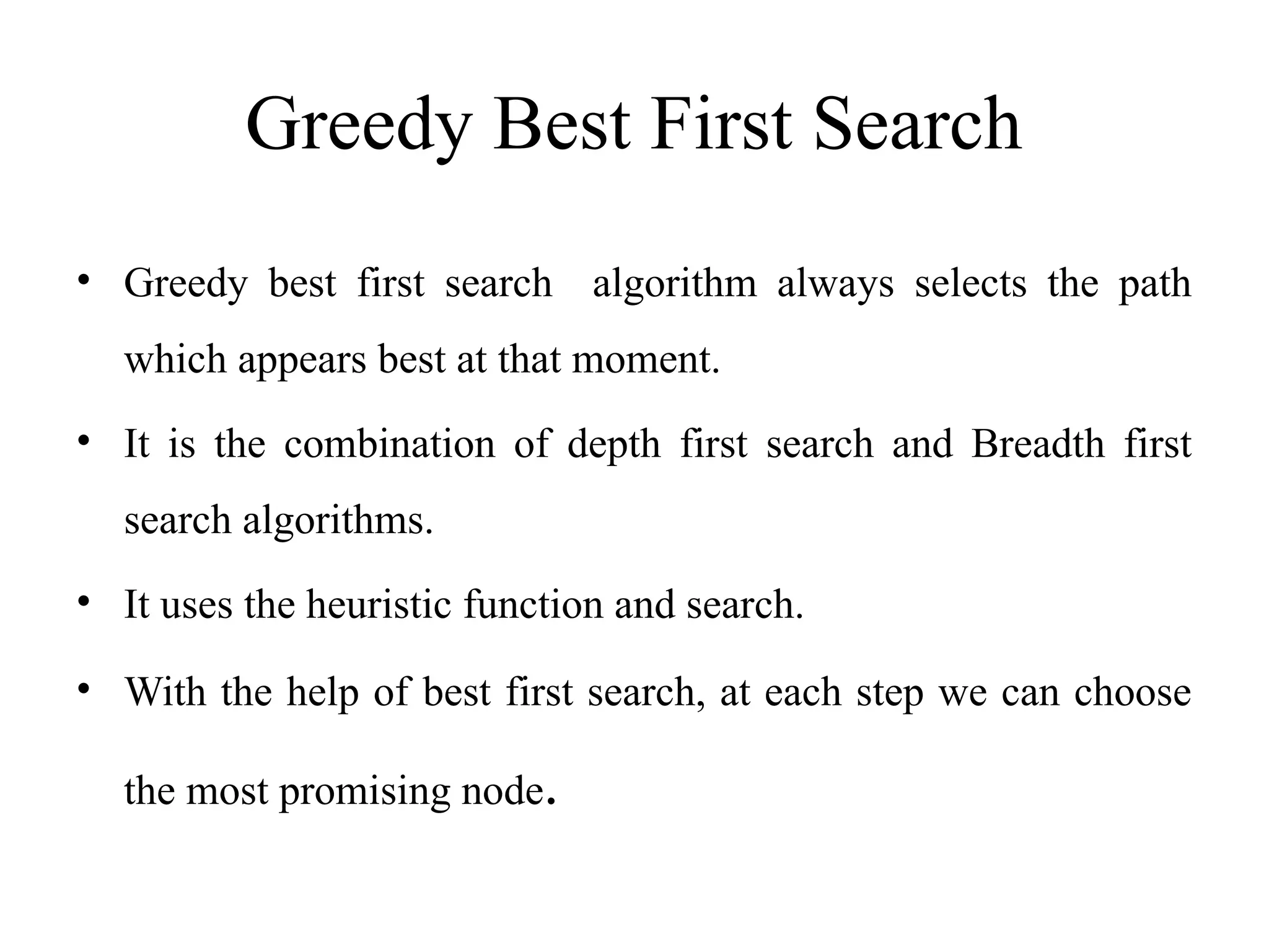
52. Greedy Best First Search
• Greedy best first search algorithm always selects the path
which appears best at that moment.
• It is the combination of depth first search and Breadth first
search algorithms.
• It uses the heuristic function and search.
• With the help of best first search, at each step we can choose
the most promising node.

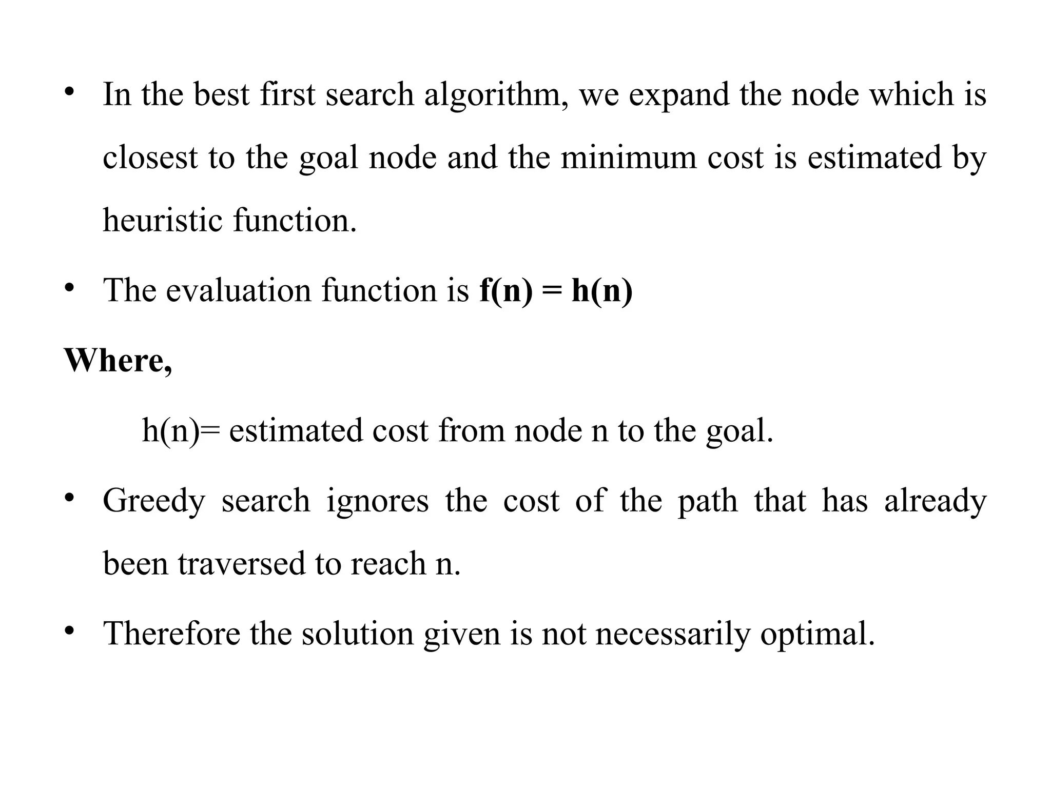
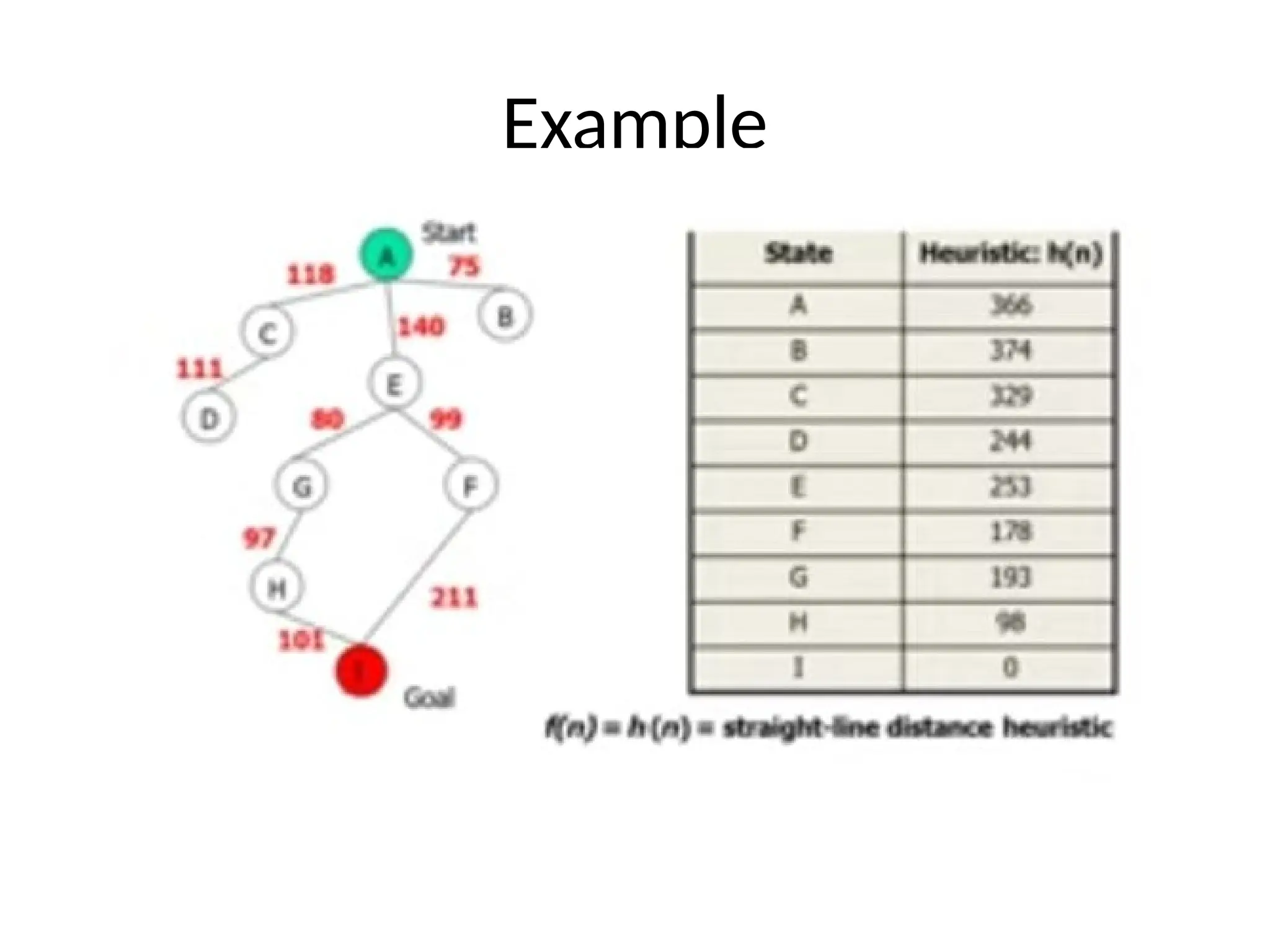
53. • In the best first search algorithm, we expand the node which is
closest to the goal node and the minimum cost is estimated by
heuristic function.
• The evaluation function is f(n) = h(n)
Where,
h(n)= estimated cost from node n to the goal.
• Greedy search ignores the cost of the path that has already
been traversed to reach n.
• Therefore the solution given is not necessarily optimal.

54. Example

55. A
C E B
Start
118
140
75
[329] [374]
[253]
G A F
[193]
[366] [178]
80 99
I
E
[253] [0]
211
Goal
Path cost is A-E-F-I = 253 +178+0 =431
Dist A-E-F-I=140+99+211 =450

56. • Optimality: Not optimal
• Completeness : In complete
• Time and space complexity of greedy search
are both O(bm
)
Where,
b is the branching factor
m is the maximum path length.

57. A* Search Algorithm
• A* search is the most commonly known form of best-first search.
• It uses heuristic function h(n), and cost to reach the node n from the start
state g(n).
• Greedy best first search is efficient but it is not optimal and not complete.
• Uniform cost search minimizes the cost g(n) from the initial state n. it is
optimal but not efficient.
• It has combined features of UCS and greedy best-first search, by which it
solve the problem efficiently.
• A* search algorithm finds the shortest path through the search space
using the heuristic function.
• This search algorithm expands less search tree and provides optimal
result faster.
• A* algorithm is similar to UCS except that it uses g(n)+h(n) instead of
g(n).

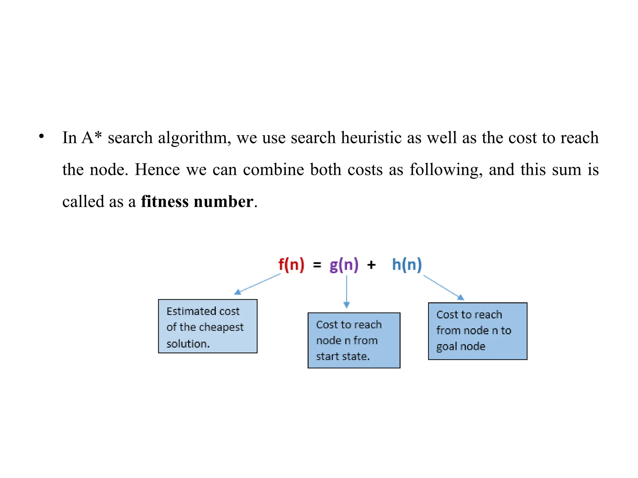
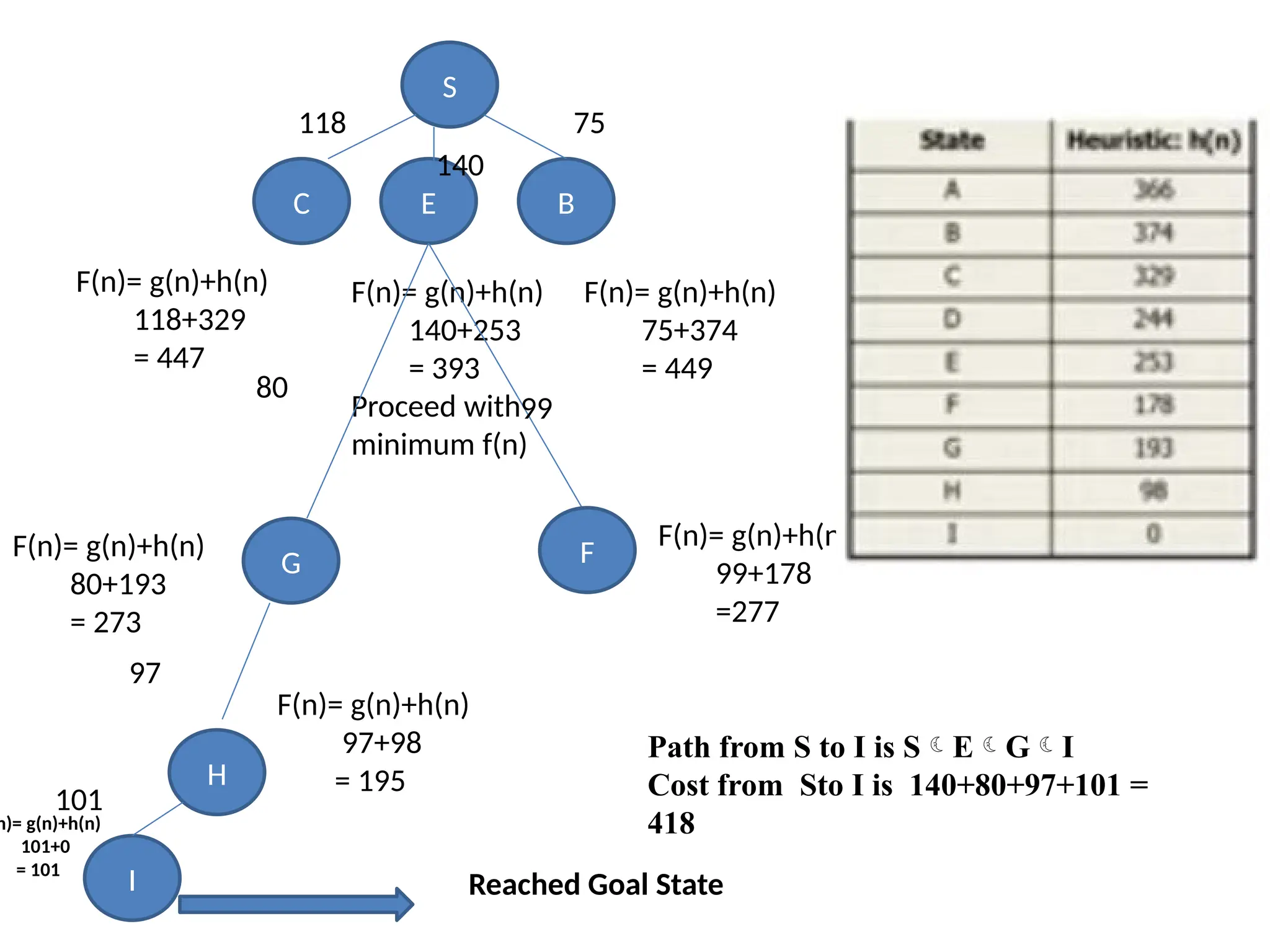
58. • In A* search algorithm, we use search heuristic as well as the cost to reach
the node. Hence we can combine both costs as following, and this sum is
called as a fitness number.

59. Example

60. S
B
E
C
118
140
75
F(n)= g(n)+h(n)
118+329
= 447
F(n)= g(n)+h(n)
140+253
= 393
Proceed with
minimum f(n)
F(n)= g(n)+h(n)
75+374
= 449
G F
F(n)= g(n)+h(n)
80+193
= 273
F(n)= g(n)+h(n)
99+178
=277
H
F(n)= g(n)+h(n)
97+98
= 195
Path from S to I is SEGI
Cost from Sto I is 140+80+97+101 =
418
80
99
97
I
101
n)= g(n)+h(n)
101+0
= 101
Reached Goal State

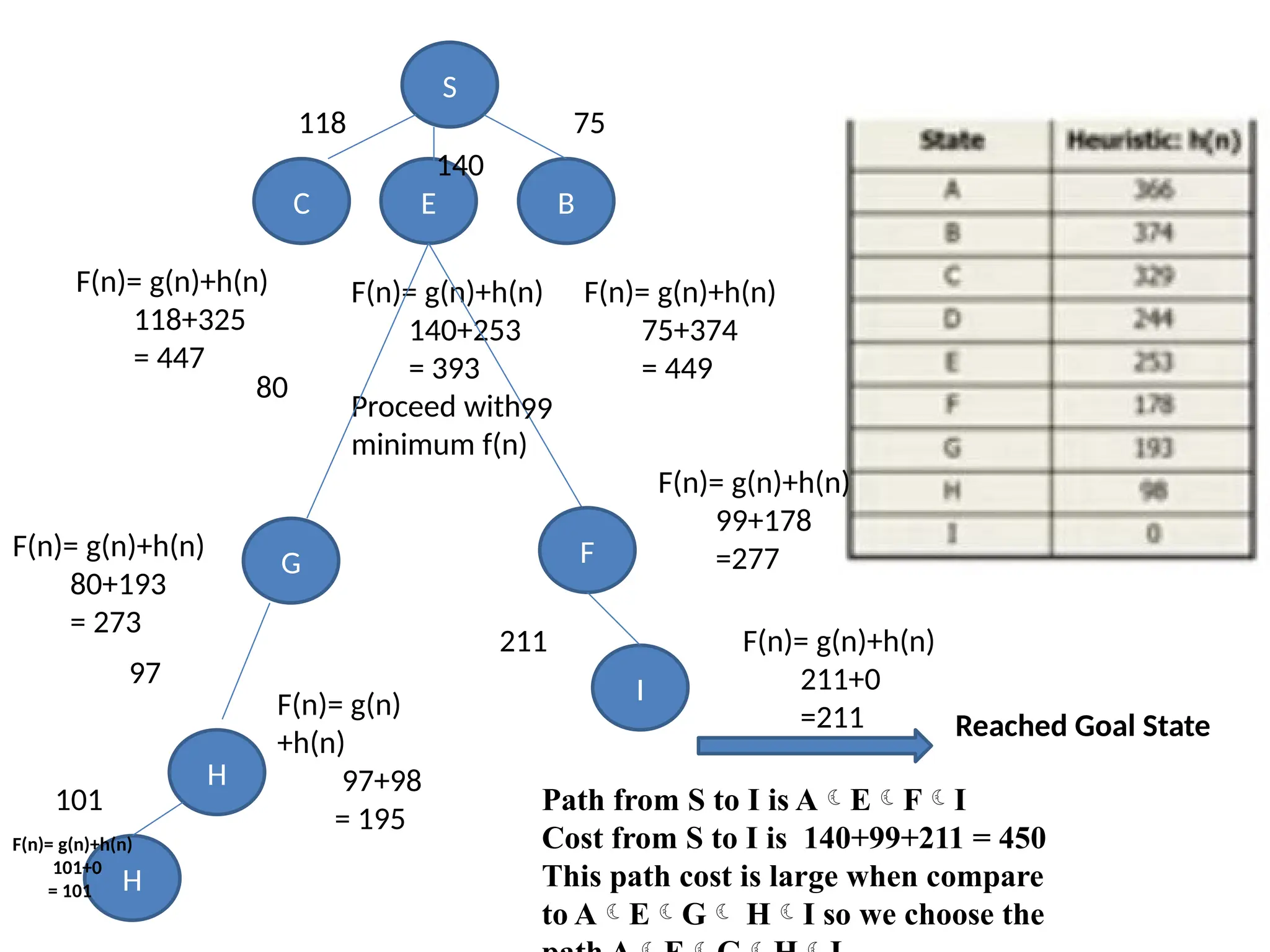
61. S
B
E
C
118
140
75
F(n)= g(n)+h(n)
118+325
= 447
F(n)= g(n)+h(n)
140+253
= 393
Proceed with
minimum f(n)
F(n)= g(n)+h(n)
75+374
= 449
G F
F(n)= g(n)+h(n)
80+193
= 273
F(n)= g(n)+h(n)
211+0
=211
H
F(n)= g(n)
+h(n)
97+98
= 195
Path from S to I is AEFI
Cost from S to I is 140+99+211 = 450
This path cost is large when compare
to AEG HI so we choose the
80
99
97
H
101
F(n)= g(n)+h(n)
101+0
= 101
Reached Goal State
I
F(n)= g(n)+h(n)
99+178
=277
211

62. • Optimality: optimal
• Completeness : complete
• Time and space complexity of A* algorithm
are both O(bm
)

63. function RECURSIVE-BEST-FIRST-SEARCH(problem) returns a solution, or failure
RBFS(problem,MAKE-NODE(problem.INITIAL-STATE),∞)
function RBFS(problem, node, f limit ) returns a solution, or failure and a new f-cost limit
if problem.GOAL-TEST(node.STATE) then return SOLUTION(node)
successors ←[ ]
for each action in problem.ACTIONS(node.STATE) do
add CHILD-NODE(problem, node, action) into successors
if successors is empty then return failure,∞
for each s in successors do /* update f with value from previous search, if any */
s.f ← max(s.g + s.h, node.f )
loop do
best ←the lowest f-value node in successors
if best .f > f limit then return failure, best .f
alternative ←the second-lowest f-value among successors
result , best .f ←RBFS(problem, best , min( f limit, alternative))
if result _= failure then return result
Algorithm

64. Hill Climbing Algorithm in Artificial Intelligence
• Hill climbing algorithm is a local search algorithm which continuously
moves in the direction of increasing elevation/value to find the peak of
the mountain or best solution to the problem. It terminates when it
reaches a peak value where no neighbor has a higher value.
• Hill climbing algorithm is a technique which is used for optimizing the
mathematical problems. One of the widely discussed examples of Hill
climbing algorithm is Traveling-salesman Problem in which we need to
minimize the distance traveled by the salesman.
• It is also called greedy local search as it only looks to its good immediate
neighbor state and not beyond that.
• A node of hill climbing algorithm has two components which are state
and value.
• Hill Climbing is mostly used when a good heuristic is available.
• In this algorithm, we don't need to maintain and handle the search tree or
graph as it only keeps a single current state.

65. Features of Hill Climbing:
Following are some main features of Hill Climbing Algorithm:
• Generate and Test variant: Hill Climbing is the variant of
Generate and Test method. The Generate and Test method
produce feedback which helps to decide which direction to
move in the search space.
• Greedy approach: Hill-climbing algorithm search moves in
the direction which optimizes the cost.
• No backtracking: It does not backtrack the search space, as it
does not remember the previous states.

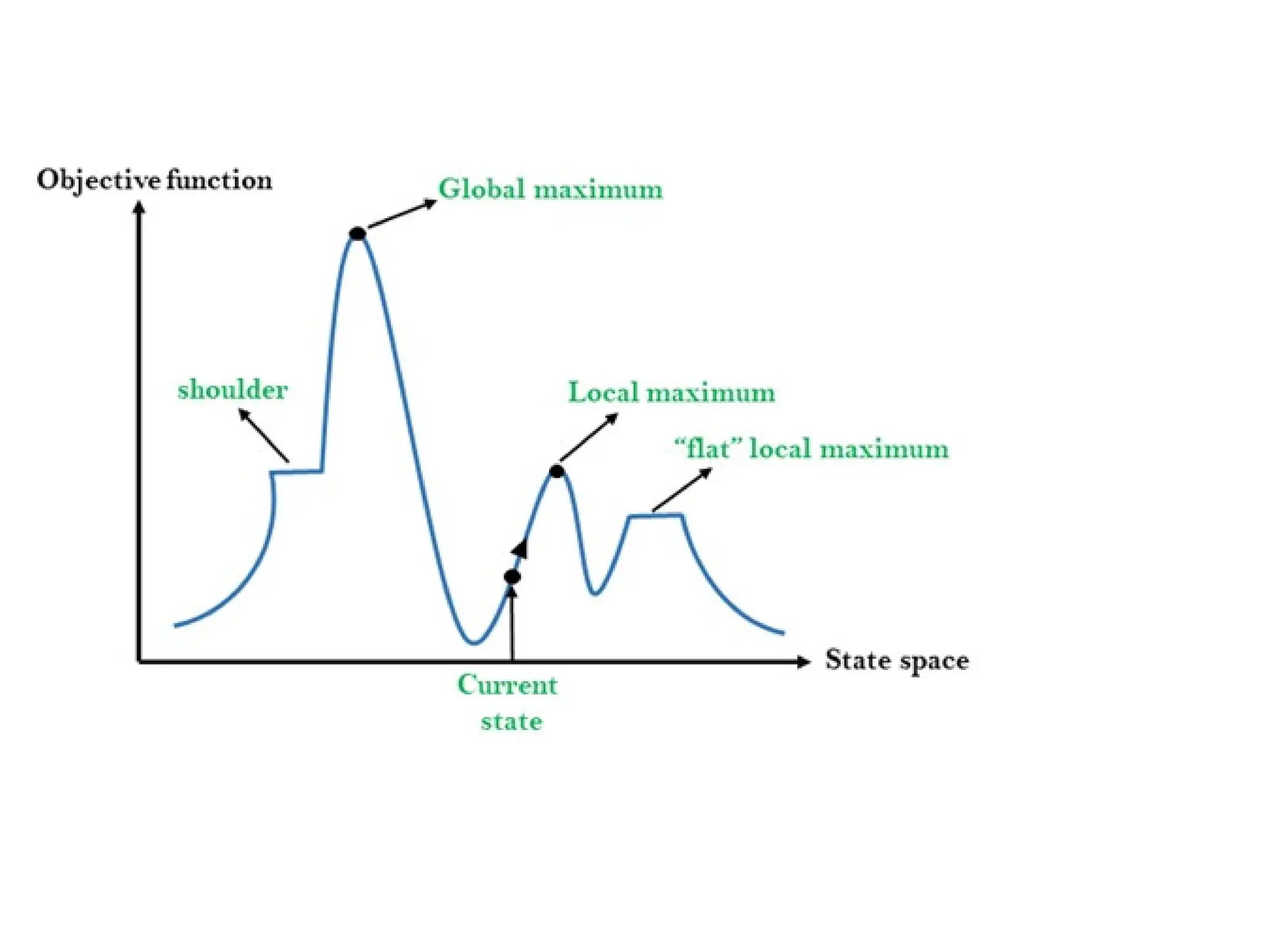
66. State-space Diagram for Hill Climbing:
• The state-space landscape is a graphical representation of the
hill-climbing algorithm which is showing a graph between
various states of algorithm and Objective function/Cost.
• On Y-axis we have taken the function which can be an
objective function or cost function, and state-space on the x-
axis. If the function on Y-axis is cost then, the goal of search is
to find the global minimum and local minimum. If the
function of Y-axis is Objective function, then the goal of the
search is to find the global maximum and local maximum.

67. Different regions in the state space landscape
• Local Maximum: Local maximum is a state which is better
than its neighbor states, but there is also another state which
is higher than it.
• Global Maximum: Global maximum is the best possible
state of state space landscape. It has the highest value of
objective function.
• Current state: It is a state in a landscape diagram where an
agent is currently present.
• Flat local maximum: It is a flat space in the landscape where
all the neighbor states of current states have the same value.
• Shoulder: It is a plateau region which has an uphill edge.

69. Types of Hill Climbing Algorithm:
• Simple hill Climbing:
• Steepest-Ascent hill-climbing:
• Stochastic hill Climbing:

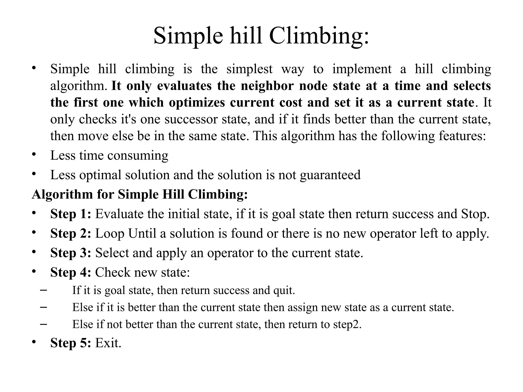
70. Simple hill Climbing:
• Simple hill climbing is the simplest way to implement a hill climbing
algorithm. It only evaluates the neighbor node state at a time and selects
the first one which optimizes current cost and set it as a current state. It
only checks it's one successor state, and if it finds better than the current state,
then move else be in the same state. This algorithm has the following features:
• Less time consuming
• Less optimal solution and the solution is not guaranteed
Algorithm for Simple Hill Climbing:
• Step 1: Evaluate the initial state, if it is goal state then return success and Stop.
• Step 2: Loop Until a solution is found or there is no new operator left to apply.
• Step 3: Select and apply an operator to the current state.
• Step 4: Check new state:
– If it is goal state, then return success and quit.
– Else if it is better than the current state then assign new state as a current state.
– Else if not better than the current state, then return to step2.
• Step 5: Exit.

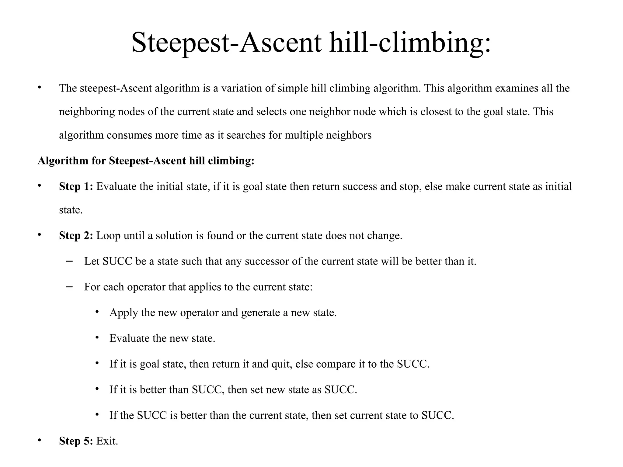
71. Steepest-Ascent hill-climbing:
• The steepest-Ascent algorithm is a variation of simple hill climbing algorithm. This algorithm examines all the
neighboring nodes of the current state and selects one neighbor node which is closest to the goal state. This
algorithm consumes more time as it searches for multiple neighbors
Algorithm for Steepest-Ascent hill climbing:
• Step 1: Evaluate the initial state, if it is goal state then return success and stop, else make current state as initial
state.
• Step 2: Loop until a solution is found or the current state does not change.
– Let SUCC be a state such that any successor of the current state will be better than it.
– For each operator that applies to the current state:
• Apply the new operator and generate a new state.
• Evaluate the new state.
• If it is goal state, then return it and quit, else compare it to the SUCC.
• If it is better than SUCC, then set new state as SUCC.
• If the SUCC is better than the current state, then set current state to SUCC.
• Step 5: Exit.

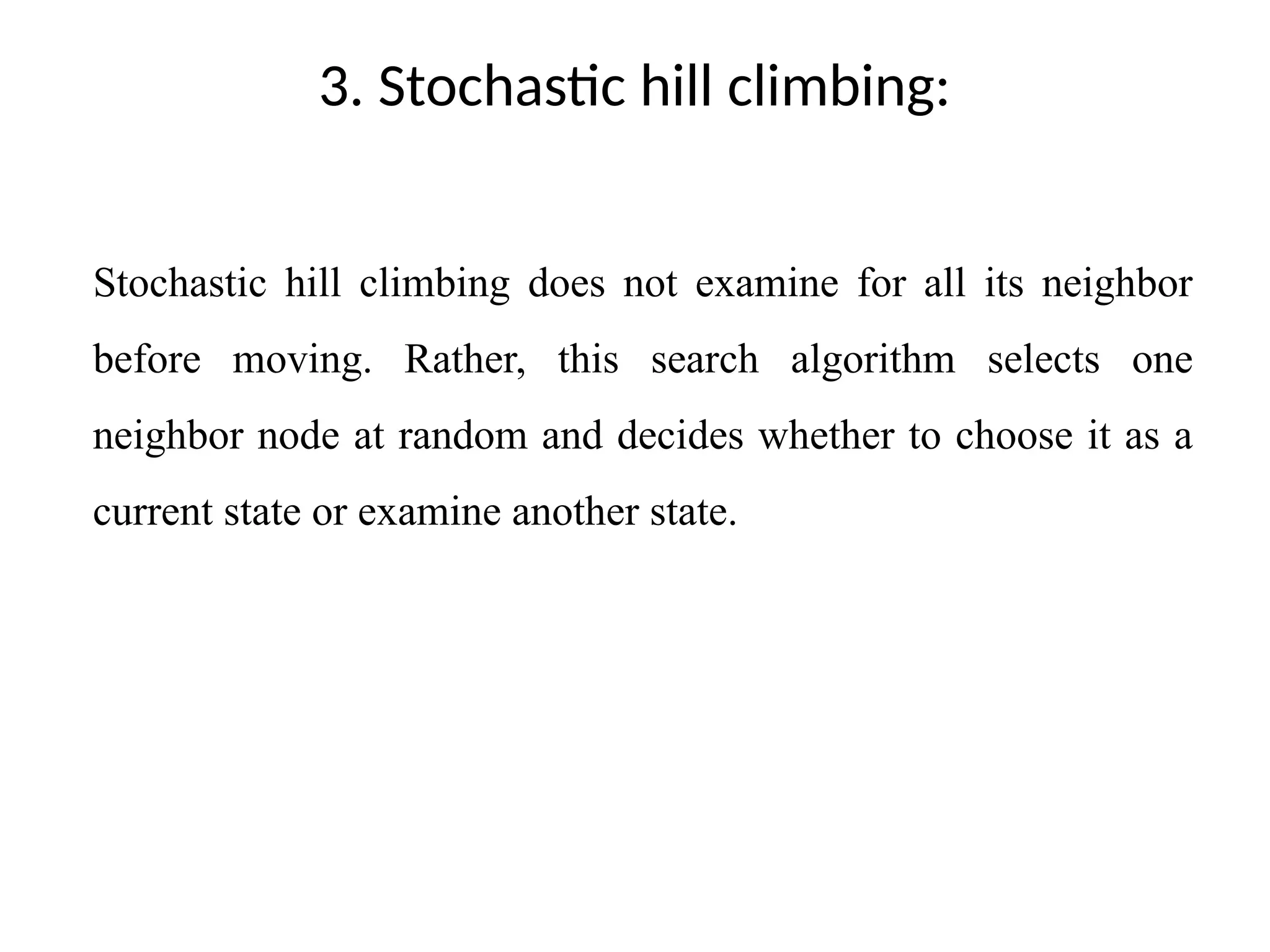
72. 3. Stochastic hill climbing:
Stochastic hill climbing does not examine for all its neighbor
before moving. Rather, this search algorithm selects one
neighbor node at random and decides whether to choose it as a
current state or examine another state.