ch4

1
4. The Electoral Effects of Fiscal Policies
Do voters reward or punish incumbent governments for expansionary budgetary measures –
cutting taxes and increasing government spending – in the years prior to elections? Similarly, do
voters sanction governments for contractionary fiscal policies? Do the electoral consequences of
fiscal adjustments depend on the balance of expenditure and revenue measures? Are voters
biased toward protecting social expenditure from the costs of adjustment? Does the extent to
which voters sanction incumbent parties for changes in fiscal outcomes depend on whether the
government is composed of a single party or coalition of parties, or whether or not the party in
government commands a majority of seats in parliament? Do voters sanction right-wing parties
differently? Are the electoral effects of budgetary measures different between incumbent
governments in new and established democracies, and between those facing reelection under
majoritarian and proportional electoral rules? Examining national-level data on fiscal and
electoral outcomes, I address each of these questions in turn, while acknowledging the need for
further research at every stage of the analysis.1
Each question lends itself to a wide range of
observational and experimental research designs at cross-national, single-country, and
subnational levels. My contribution here is simply to identify whether or not changes in the level
and composition of government expenditure and revenue are associated with changes in
incumbent party vote share in national elections.
We know remarkably little about the relationship between fiscal policies and electoral outcomes.
This is unfortunate given the current practical relevance of the topic. One can easily concoct
alternative narratives to explain the fates of incumbent parties in countries that have
implemented austerity measures to combat the borrowing costs associated with rising
government debt. Following the May 2012 election, observers of Greek politics argued that
voters punished both the opposition New Democracy and (in particular) the ruling PASOK party
(which lost 119 of its 160 seats in parliament) in the 2012 elections for agreeing to deep cuts in
government spending and tax increases mandated by creditors (Financial Times 2012; Spiegel
Online 2012; The Telegraph 2012). However, in the prior election, the ruling New Democracy
party lost 61 seats following an increase in the fiscal deficit from -6.7% of GDP to -15.3% of
GDP over the prior two years (ParlGov 2015; OECD 2015). Perhaps it was not the increase (in
2009) or decrease (in 2012) in the deficit that led voters to defect from the two dominant Greek
parties, but rather low economic growth and high unemployment spurred by a steep decline in
foreign credit during the global financial crisis of 2008 and 2009.
During the same time period, a different set of political developments took place in the
United Kingdom. In 2010, Bank of England governor Mervyn King predicted that the winner of
the general election would be “out of power for a whole generation” due to the severity of budget
cuts (The Guardian 2010a). The following week, Labour lost 91 seats – a year removed from an
1
This chapter uses data from the “Economic Voting Dataset” described in Appendix A. For data, please
email the author at donnelly.patrick.t@gmail.com.

2
unprecedented (given available data) increase in the budget deficit from -5.0% to -11.0% of GDP
(ParlGov 2015; OECD 2015). Five years later, the Conservative Party was reelected following a
similarly unprecedented succession of austerity measures.
Which narrative is correct? Do voters reward or punish governments for budget cuts? Are
voters indifferent to fiscal policies, sanctioning governments instead for changes in economic
output and unemployment? Or do the electoral consequences of fiscal adjustments depend on the
broader economic and political context? In Greece, a member of the European Economic and
Monetary Union, a center-left single-party government facing an immediate shortage of credit
presided over austerity measures mandated by international lending organizations. In the United
Kingdom, a monetarily sovereign country with the ability to borrow at relatively low rates, a
center-right coalition government presided over austerity measures without conditions imposed
by foreign creditors. Given this contextual variation, it is necessary to expand the sample of
observations far beyond these two cases in order to identify the electoral effects of changes in
government revenue and expenditure.
Three prior studies have used time-series cross-sectional analysis on national-level data to
identify electoral effects, of which two measure electoral consequences using election results.
Only one uses change in incumbent party vote share to measure the extent to which voters
sanction incumbents. Brender and Drazen (2008) claim that the probability of incumbent
reelection in developed countries increases with the change in the budget deficit. Alesina,
Carloni, and Lecce (2013) contend that voters in OECD member states do not systematically
punish governments for implementing fiscal adjustments. However, using vote share rather than
a binary indicator of reelection or change in cabinet ideology, Nyman (2014) finds that
incumbents’ electoral prospects decrease with the structural budget balance. As I will show later
in this chapter, the basic results of these studies fail to replicate using a sample of available data
on fiscal variables and elections in high-income democracies. Moreover, none of the studies
attempt to estimate the effect of election-year changes in fiscal variables on changes in
government vote share – arguably the effect which best identifies the electoral consequences of
budgetary expansions and contractions.
The lack of research on the fiscal determinants of incumbent reelection prospects weakens
the credibility of theories that assume that governments are necessarily, generally, or
conditionally punished for either fiscal adjustment or welfare retrenchment. A classic
formulation of the “political budget cycle” theory contends that governments will attempt to
maximize vote share using expansionary fiscal policy prior to elections, offset by contractionary
fiscal policy after elections (Rogoff 1990). This theory in turn assumes that voters favor
expansionary policies but have short retrospective time horizons. To be precise, voters may
reward expansionary fiscal policies not because voters favor spending and oppose taxes per se,
but also because expansionary fiscal policies may indirectly increase the personal income of the
median voter by increasing aggregate demand. This assumes in turn that short-term output
increases with the budget deficit, which may not be true in general (Giavazzi and Pagano 1990),
or for expenditure-based adjustments (Alesina and Ardagna 2010), though subsequent research

3
from the International Monetary Fund (Guajardo, Leigh, and Pescatori 2011) casts doubt on the
validity of the “expansionary fiscal contraction” hypothesis.
One of the most-cited articles in the cross-national study of social policy asserts that
governments perceive welfare retrenchment as electorally costly, and thus avoid claiming
responsibility for cuts (Pierson 1996). This assumes that voters punish governments for cuts to
social programs, an assumption which subsequent research has challenged (Armingeon and
Giger 2008; Giger and Nelson 2010), using data on changes in benefit generosity as coded in
Scruggs (2004) rather than the level of expenditure. However, it is unclear whether the
retrenchment in question takes the form of fiscal adjustment (a reduction in social expenditure
without a corresponding increase in non-social expenditure or reduction in taxation), a revenue-
neutral reduction in social expenditure offset by a corresponding reduction in taxation, or a
revenue-neutral reduction in social expenditure offset by a corresponding increase in non-social
expenditure. These three forms of retrenchment have plausibly distinct electoral consequences,
each of which I will attempt to identify in the analysis.
Data and sample
In this section, I describe two ways in which researchers have measured electoral outcomes.
The most-cited study of the electoral effects of deficits uses a binary measure of incumbent
electoral success. An alternative approach, frequently used to identify the electoral effects of
macroeconomic conditions, calculates the change in vote share between elections for the
incumbent party. I advocate using the change in vote share, which is more accurate and precise
than the binary measure. To support this claim, I give specific instances in which the binary
variable erroneously measures electoral success or failure. Later, I will show more generally that
using the binary measure tends to produce biased estimates of the electoral consequences of
deficits.
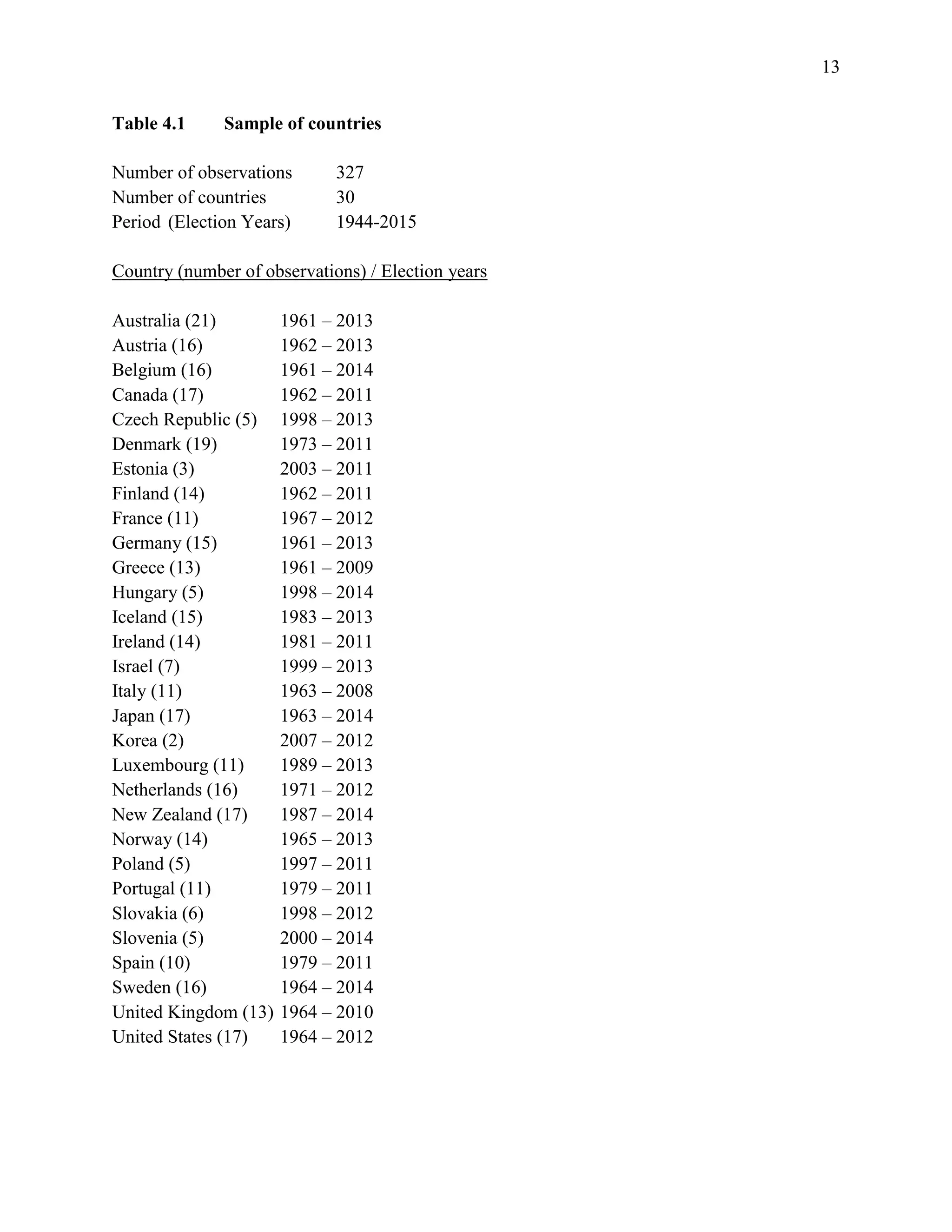
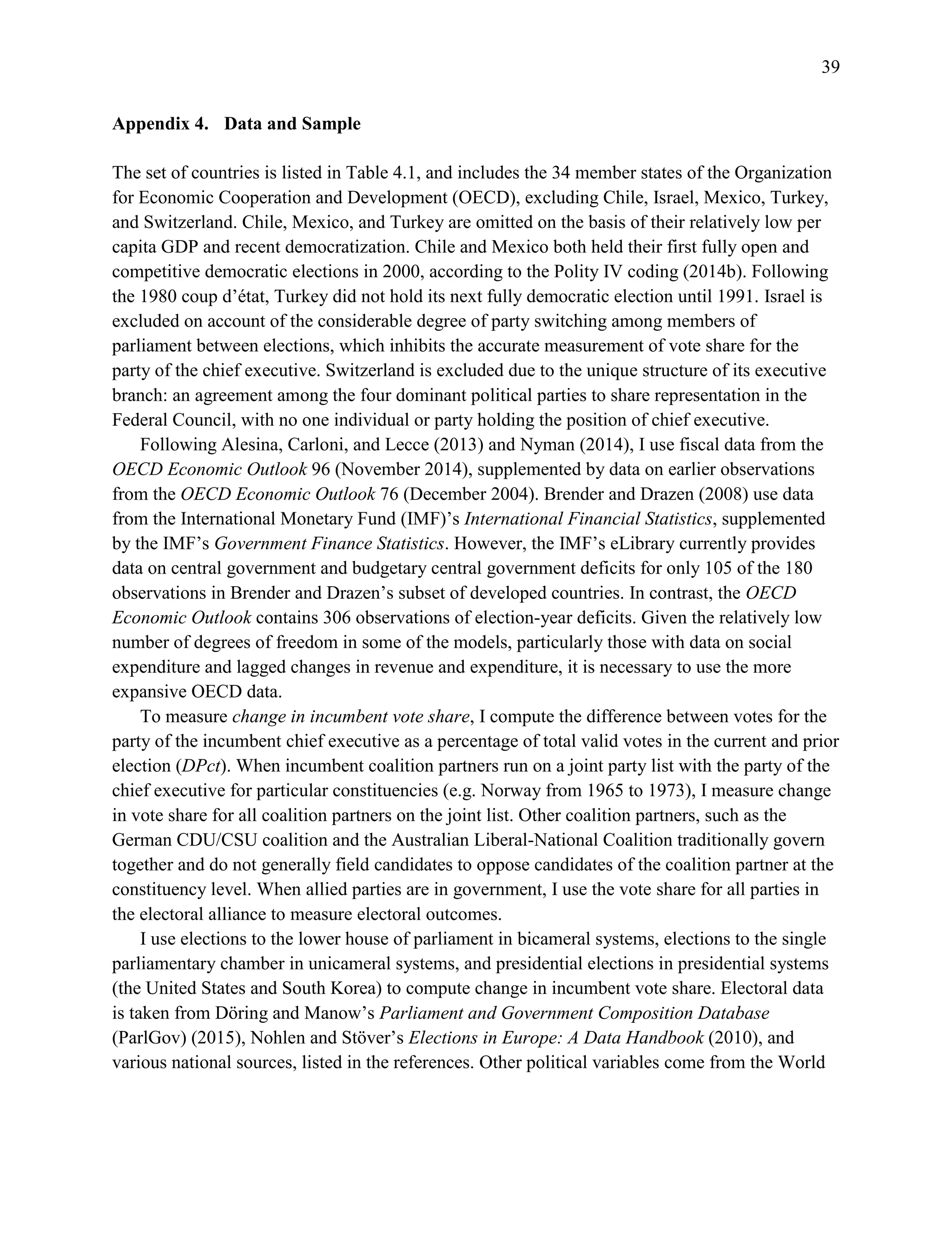
The sample consists of 355 democratic elections contested between 1948 and May 2015. For
a detailed description of the sample, and of other variables included in the analysis, see
Appendix 4. Table 4.1 lists the election years and number of observations for all countries in the
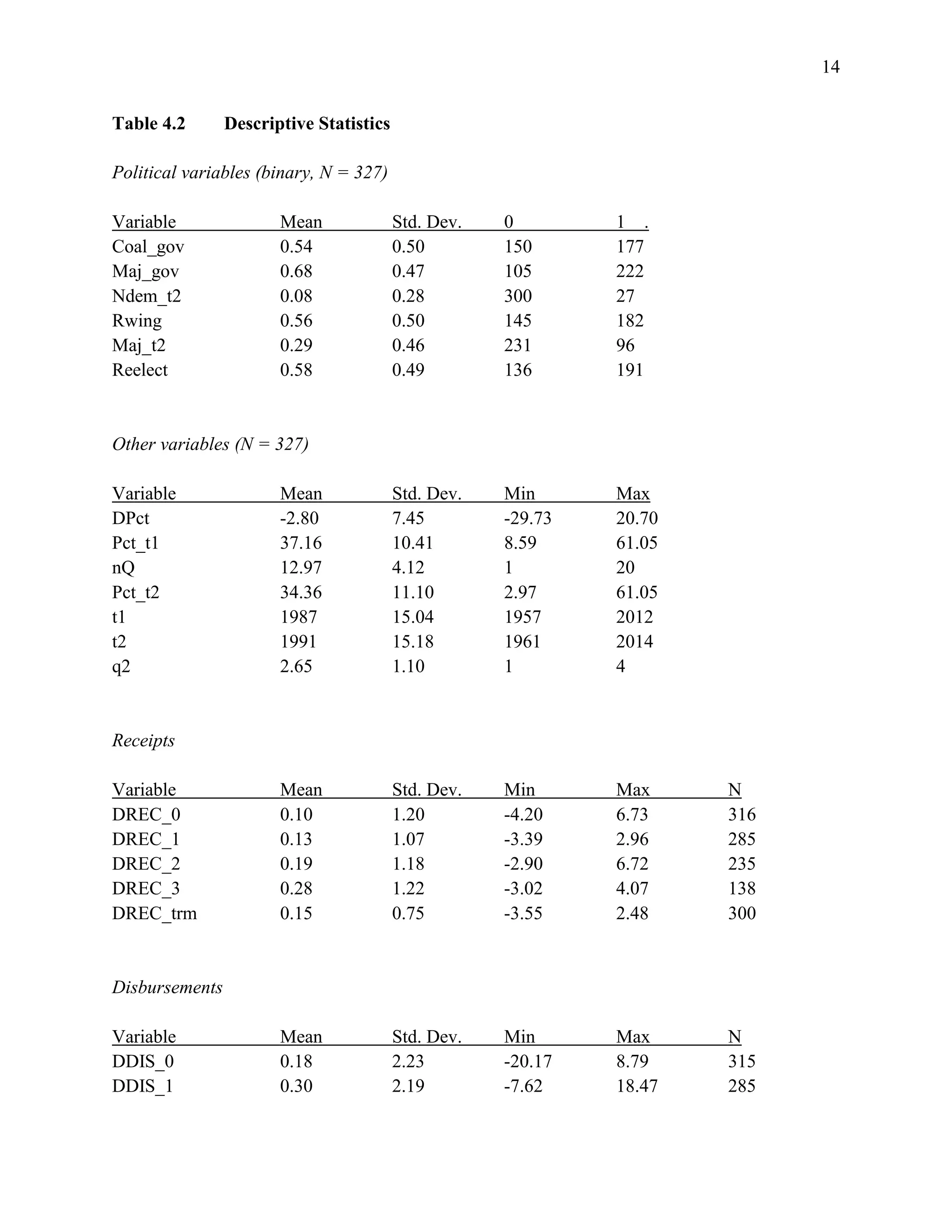
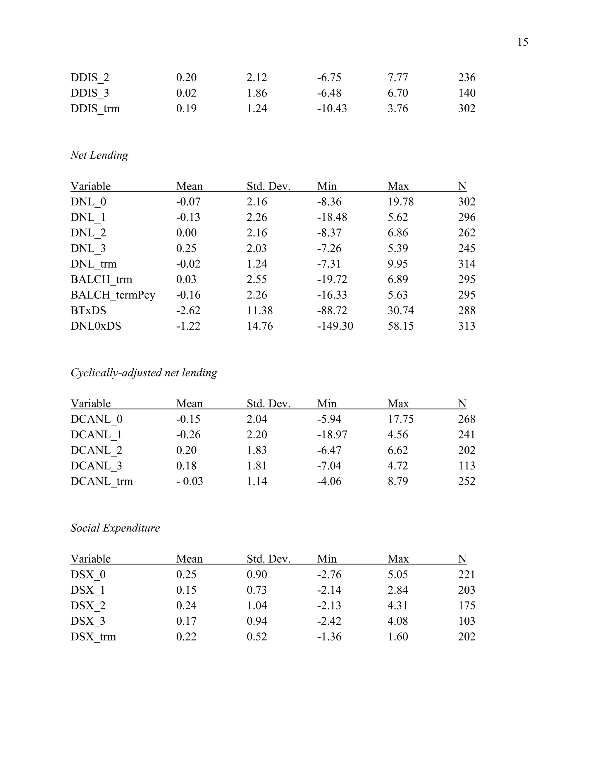
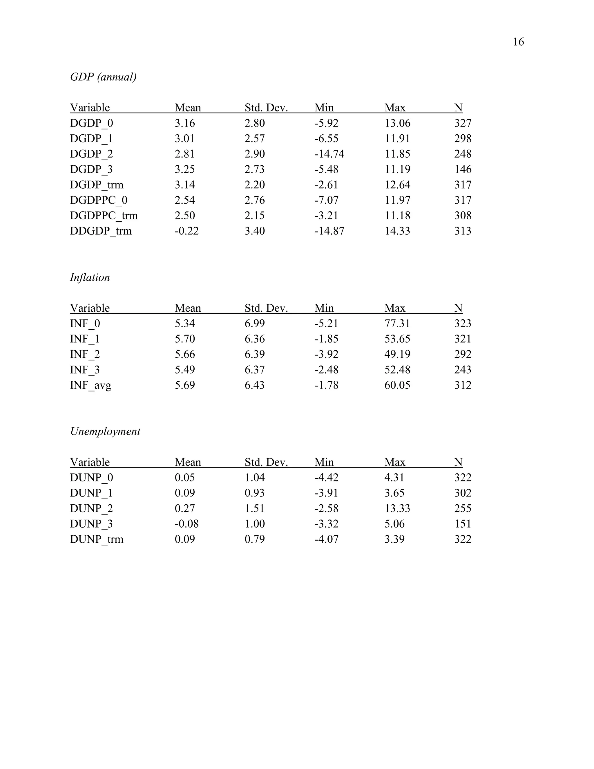
sample. Table 4.2 presents descriptive statistics of each of the variables used in the statistical
models.
[Tables 4.1-4.2 here]
The response variable in each model is a measure of incumbent party electoral performance:
either a binary indicator of reelection (Reelect), equal to 1 if the party of the incumbent chief
executive is reelected and 0 otherwise; or a continuous measure of change in incumbent vote
share (DPct). Nyman (2014) suggests that incumbent governments may be more likely to
implement unpopular fiscal measures when they perceive that their loss in vote share will not
cost them reelection. This assumes that governments can adequately identify the prospective

4
electoral costs or benefits of fiscal policies and will enact preferred policies subject to the
constraint of reelection, rather than choosing the policies that they perceive will maximize vote
share.
By measuring the extent to which voters expand or withdraw support for incumbent parties,
rather than whether or not voters’ change in support for incumbents leads to reelection, DPct is
an infinitely more precise measure of incumbent electoral performance than Reelect. To take the
most extreme examples, using the Reelect variable as a measure of incumbent party success or
failure would indicate that voters “rewarded” the Progressive Conservative Party of Canada in
1962 with a withdrawal of support of 16.4% of total votes, enough to sustain an eight-month
minority government after governing with over 78% of seats in the House of Commons during
the prior term! At the other extreme, voters “punished” Fidesz in the 2002 Hungarian elections
with an increase in vote share of 12.9%, insufficient to overcome a similar increase in vote share
for the opposition MSZP at the expense of minor parties. The Hungarian example highlights a
limitation of estimating changes in vote share using support for the party of the chief executive,
rather than all parties in government.
Besides more precisely measuring voters’ reactions to changes in the level and composition
of government expenditure and revenue, DPct more accurately captures the direct electoral
consequences of fiscal expansions and contractions. Bargaining over the allocation of cabinet
portfolios affects whether or not the incumbent party retains power following parliamentary
elections in multiparty systems. In some cases, such as Italy throughout the 1980s, the dominant
party (e.g. Christian Democracy) may agree to support a government headed by a prime minister
of a party with substantially less electoral support (e.g. the Italian Socialist Party).
Moreover, when incumbent parties have a large initial degree of support – such as the Liberal
Democratic Party during much of postwar Japanese history – using a binary reelection indicator
is unlikely to capture variation in incumbent electoral support, and may inaccurately suggest that
voters are not sanctioning incumbent governments for their policies. In contrast, DPct simply
measures the extent to which voters extend or withdraw support for the incumbent party.
Perhaps for this reason, economic voting models tend to use change in incumbent vote share
rather than binary indicators of reelection to measure electoral outcomes (Lewis-Beck and
Stegmaier 2000; Paldam 1991; Powell and Whitten 1993).
In the next section, I replicate the basic models of Brender and Drazen (2008), and Nyman
(2014). I do not replicate Alesina, Carloni, and Lecce’s models, which estimate the annual effect
of changes in the (structural) budget balance on changes in cabinet ideology. In this chapter, I am
strictly interested in the effect of fiscal expansion or contraction on electoral performance in
subsequent elections. However, Alesina et al. identify variables which may confound the
relationship between changes in the budget deficit and changes in electoral outcomes, two of
which I include as control variables in my analysis. The authors include dichotomous political
variables indicating whether or not the incumbent administration is a coalition government
(Coal_gov) or majority government (Maj_gov), as well as a continuous variable measuring the
number of (continuous) years that the incumbent has held office, including the current year.

5
In some cases, the prime minister is initially elected with the support of a majority of
members of parliament, but later loses majority support while retaining office prior to the
subsequent election. In other cases, minority governments gain majority support between
elections. Some cabinets gain and lose majority support more than once during an election cycle.
In coding the majority government variable, I measure majority status at the end of each quarter,
except for q2, in which majority status is measured at the time of election. If an election is called
immediately after a government loses majority support, I code the government at t2 as a majority
government. Additionally, since voters may be less likely to support incumbents with a longer
tenure in office (Romer 2013), I include a variable in each of my original models measuring
government duration in quarters (nQ).
Brender and Drazen (2008) argue that systematic political budget cycles are limited to new
democracies (see also Brender and Drazen 2005), and thus define a binary variable for all
observations in the first four post-transition election cycles. I include this variable in my dataset.
The authors also include a majoritarian electoral system variable in their models to control for
potentially heterogeneous effects between governments (indirectly, in parliamentary systems)
elected under plurality rule and proportional representation. Each of these variables is measured
at the time of the second election for each election cycle.
Nyman (2014) includes a variable indicating whether or not the party in government
(presumably that of the chief executive) is right-wing. Nyman argues that voters are less likely to
punish right-wing as opposed to less-wing parties for contractionary fiscal policies, since the
distributional costs of fiscal adjustment are typically borne by lower-income citizens. The
assumption is that right-wing parties are more likely to benefit electorally for fiscal policies that
benefit higher-income voters, while the reelection prospects of left-wing parties increase when
budgetary measures lead to a more equal distribution of income or wealth. Similarly, if voters
reward governments for contractionary fiscal policies, right-wing parties may electorally benefit
to a greater extent than their left-wing counterparts for implementing fiscal adjustments.
Voters may also be more likely to punish right-wing governments for tax increases than left-
wing governments. If right-wing parties typically prefer lower taxes and lower government
spending, voters may withdraw their support for right-wing governments for breaking promises
outlined in their electoral platforms. The possibility of partisan effects may thus justify inclusion
of a variable indicating partisan identification, and in any event the inclusion of such a variable is
necessary to replicate Nyman’s basic model. I code an incumbent party as right-wing (Rwing) if
it is defined in the Manifesto Project Database (MPD) (Budge et al. 2001; Klingemann et al.
2006; Volkens et al. 2014a) as liberal, Christian democratic, conservative, or nationalist. I make
one correction to the MPD’s coding, classifying the Portuguese Social Democratic Party as right-
wing. For electoral alliances, I classify the government as right-wing if a majority of members of
parliament in the alliance belong to right-wing parties.

6
Replication
Following the approach taken in Chapters Two and Three, I first attempt to replicate the
conclusions of Brender and Drazen’s analysis. In Models 1 and 2, the authors include variables
measuring the change in central government budget balance from the third and fourth year prior
to election to the two years prior to election (BALCH_trm), the election year change in budget
balance (DNL_0), and the change in GDP per capita over the chief executive’s term in office
(DGDPPC_trm). The authors include binary variables indicating whether or not elections were
held under majoritarian electoral rules (Maj_t2), or were one of the first four elections held since
democratic transition (Ndem_t2). Model 1 is estimated without country fixed effects. Model 2 is
estimated with fixed effects. The response variable in both models (Reelect) indicates whether or
not the party of the chief executive is reelected. As in Brender and Drazen (2008), both Models 1
and 2 are estimated by logistic regression (logit) with heteroscedasticity-consistent standard
errors.
Following Nyman (2014), I examine whether substituting a variable measuring the difference
in incumbent vote share between elections for the binary reelection indicator changes the
estimated effects of fiscal variables on reelection prospects. Since incumbents with a higher
initial vote share are more likely to lose votes between elections, I include a variable (Pct_t1)
measuring incumbent vote share from the previous election. I estimate Model 3 using ordinary
least squares regression with country-level fixed effects and heteroscedasticity-consistent
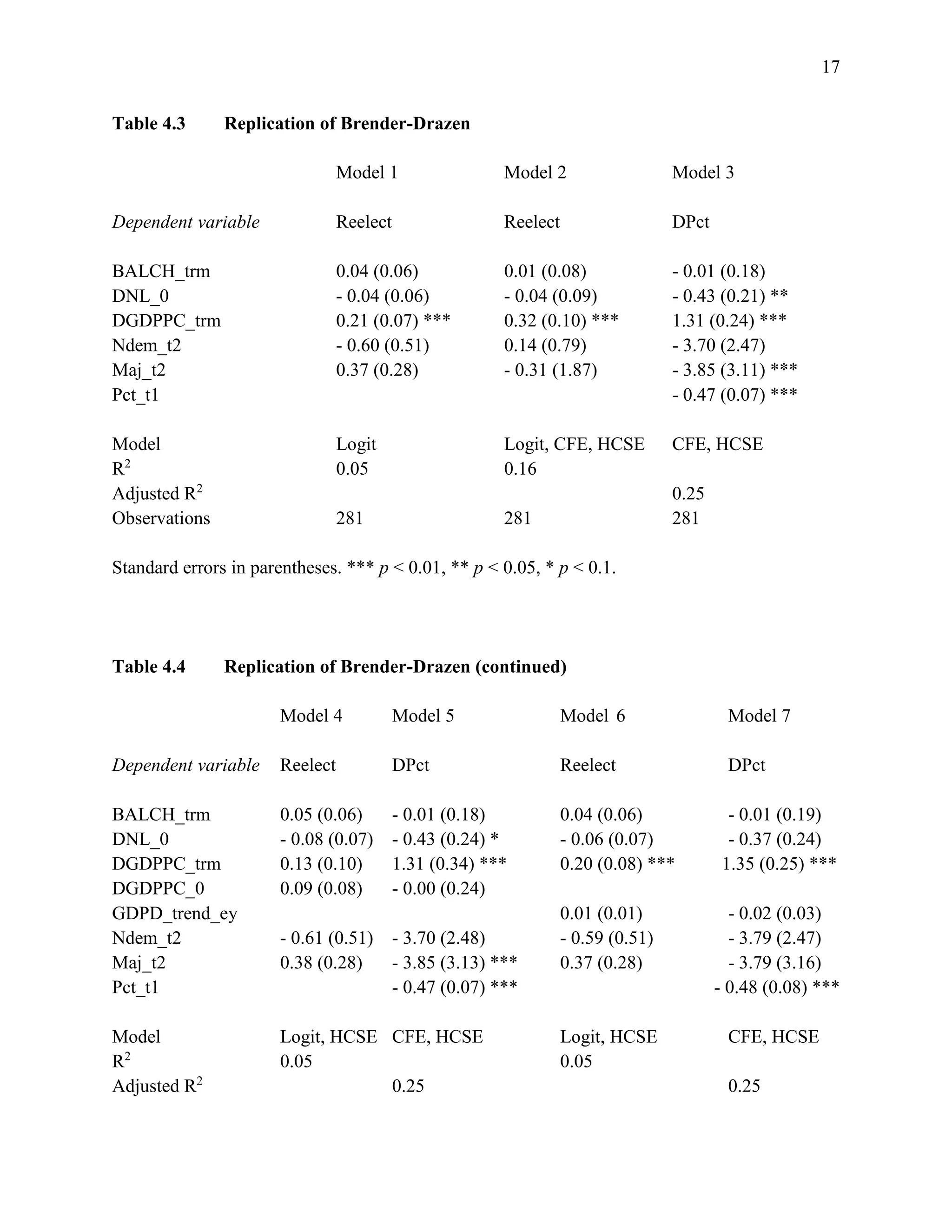
standard errors. Table 4.3 presents my initial replication of Brender and Drazen’s models.2
[Table 4.3 here]
Table 4.3 provides additional support for Brender and Drazen’s claim that the probability of
incumbent reelection increases with the change in GDP per capita. However, the authors’
conclusion that deficits inhibit reelection does not replicate for the sample of countries examined
here. Using both the binary and continuous measure of electoral performance, I find instead that
inter-election changes in the budget balance have no significant effect on reelection prospects.
More notably, the change in incumbent vote share decreases with the budget balance, directly
contradicting the authors’ finding that voters in developed countries “do not like deficits,
particularly in election years” (Brender and Drazen 2008, p. 2215).
One possibility is that the authors’ findings are sensitive to the selection of countries and
time period. Brender and Drazen define countries (more restrictively) as “developed” if they
were members of the OECD prior to 1974. Hence they include Mexico and Turkey in their
sample of developed countries, but exclude South Korea and the former Eastern Bloc countries.
Their sample covers many of the same elections from 1961 to 2003, but includes observations
for which OECD data is not available, and excludes observations after 2003.
2
I report R2
as 1 – RSS/MSS for the logit models, and the adjusted R2
for the fixed effects regressions.

7
In Models 4 through 7, I replicate Brender and Drazen’s estimates of the electoral
consequences of changes in the government budget balance, controlling for election-year
changes in economic output. Again, I find that voters generally favor looser fiscal policies in the
year of election. Changes in the budget balance over the course of the election term have no
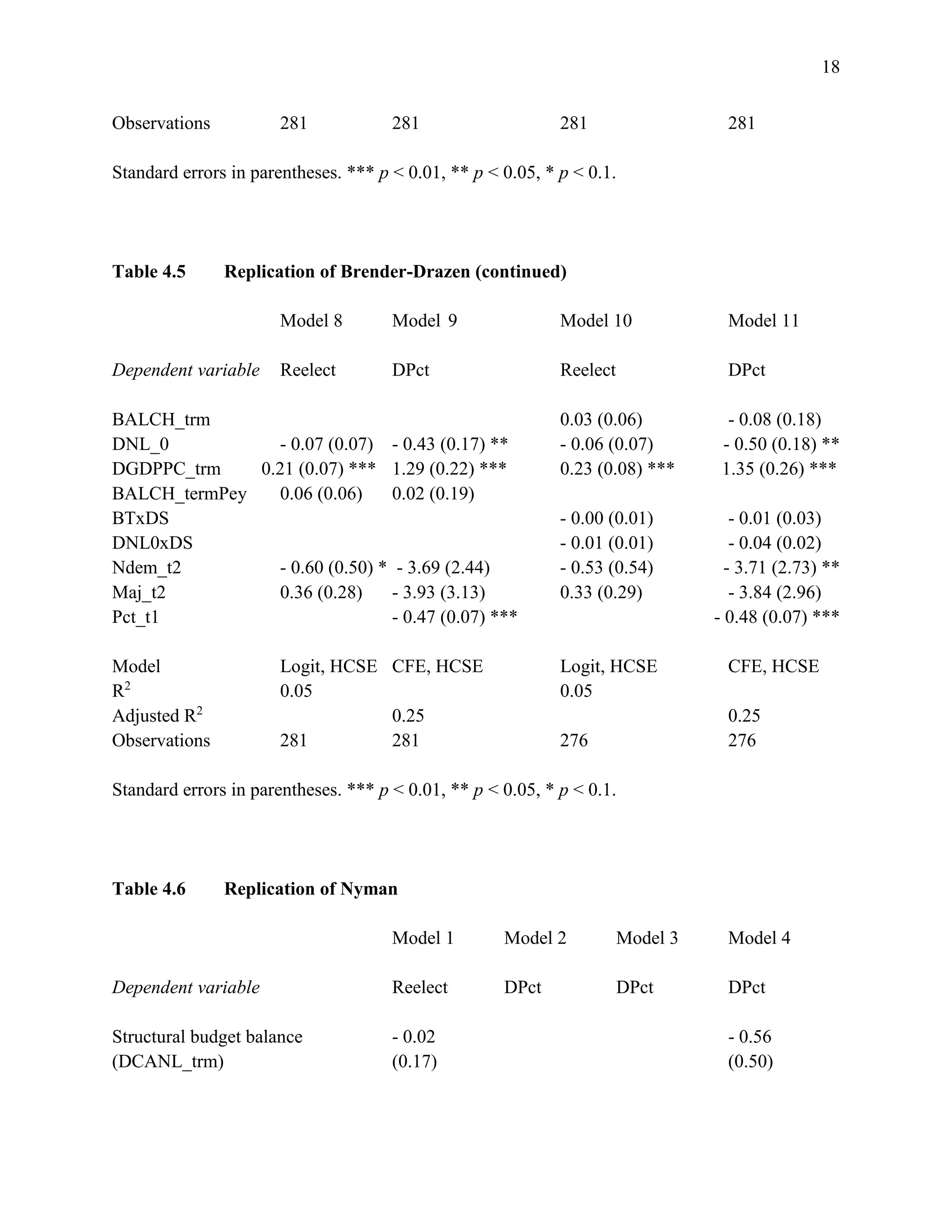
significant effect on reelection. Models 8 through 11 add alternative statistical controls but yield
the same conclusions.
[Tables 4.4 – 4.5 here]
Nyman’s basic model estimates the effect of term-length changes in the structural budget
balance on the change in incumbent vote share. Controlling for the partisan composition of
government and changes in GDP and unemployment, Nyman finds that an increase in the
general government budget balance over the course of the election cycle – with and without
cyclical adjustment – significantly corresponds to a decline in incumbent vote share (but does not
significantly affect the probability of reelection). Table 4.6 presents the estimates from my
reanalysis of Nyman’s models.
[Table 4.6 here]
Replicating Nyman’s models, I find no statistically significant relationship between the change
in the (cyclically-adjusted) budget balance and the change in the incumbent government’s vote
share. The coefficients are weaker, perhaps due to the inclusion of additional observations and
revision of prior observations from the more recent edition of the OECD Economic Outlook.
Nyman clusters standard errors at the country level, and I report heteroscedasticity-consistent
standard errors, but this cannot explain the variation in the coefficients between the authors’
estimates and the ones reported here.
Following replication of two prior studies, it is not evident that term-length changes in the
budget balance affect reelection prospects. In the following section, I provide new tests of the
hypothesis that fiscal expansions or contractions over the course of an incumbent’s term in office
significantly affects the change in incumbent party vote share. I again find no evidence that
changes in the budget balance from the prior election or change in party of the chief executive to
the current election corresponds significantly to an increase or decline in incumbent vote share.
However, I find consistent evidence that voters punish contractionary fiscal policies in election
years.
Term-length vs. election-year estimates
As the replication of Brender and Drazen’s models shows (using change in incumbent vote share
rather than a binary measure of reelection), the electoral consequences of changes in the
government budget balance depend critically on whether fiscal expansions or contractions occur
in the year of election or earlier in the term. This finding is consistent with a host of prior studies

8
on the macroeconomic determinants of electoral outcomes, which tend to show that voters are
highly myopic: they reward or punish incumbents for economic conditions in the year of election
while discounting prior changes in national, regional, or personal income. Interestingly, election-
term changes in GDP correspond significantly to changes in incumbent vote share in replication
of Brender and Drazen’s model, but election-year growth has no statistically significant effect
when controlling for term-length effects.
Political economists have used evidence of voter myopia (or assumed its existence) to
explain the presence of political business cycles and budget cycles. If voters discount economic
conditions at times that are relatively distant from the following election, then governments have
an incentive to implement expansionary fiscal (and monetary) policies prior to elections and
contractionary policies immediately after elections. Governments should thus cut taxes and
expand spending prior to elections, increasing voters’ take-home income (in the short run) and
(more controversially) expanding national income through increasing aggregate demand. In
return, voters reward governments for expansionary policies. In the following models, I provide
additional evidence that voters reward election-year fiscal expansions. The effects are consistent
across alternative model specifications, using both uncorrected and cyclically-adjusted measures
of general government net lending.
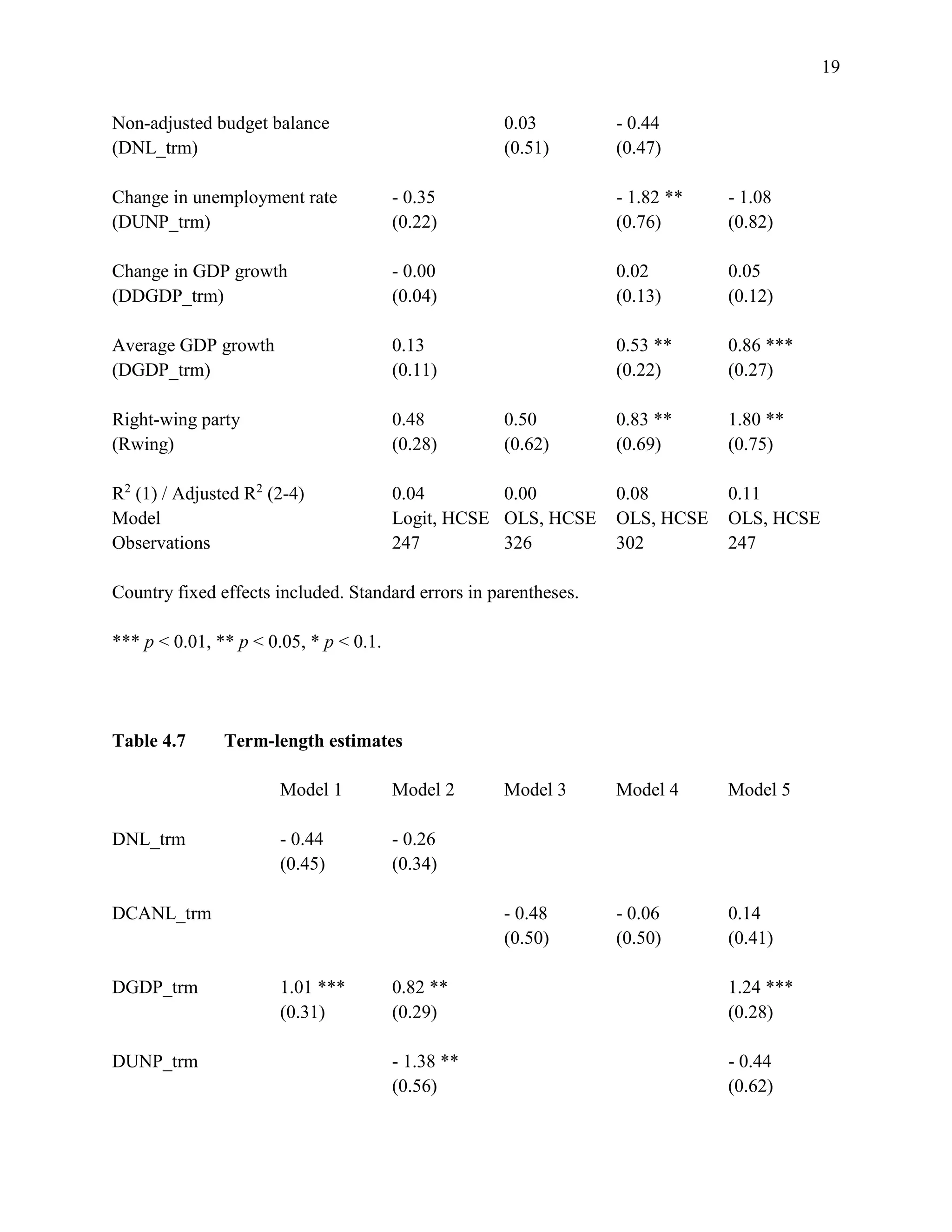
[Table 4.7 here]
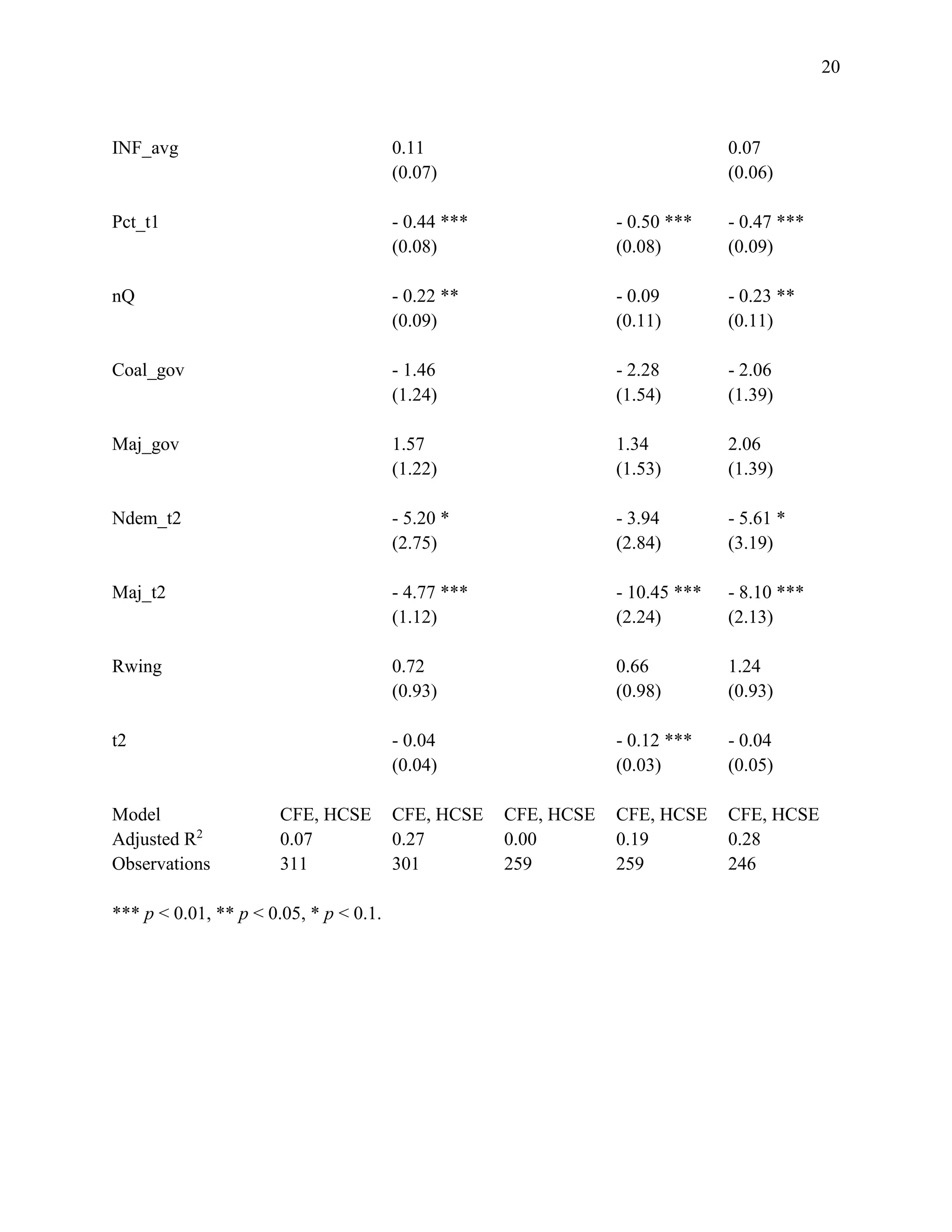
Table 4.7 shows that election-term changes in the budget deficit do not significantly affect the
vote share of incumbent governments. Although the coefficients on the net lending variables are
all negative, the standard errors are too large to conclude that term-length changes in the deficit
reduces incumbent vote share. In Model 1, I estimate term-length effects using general
government net lending (receipts less disbursements), controlling for changes in GDP. Model 2
adds additional economic and political controls. Model 3 presents the bivariate regression of
incumbent vote share on the change in cyclically-adjusted net lending. In Model 4, I add control
variables measuring the effect of potentially confounding differences in political institutions and
government characteristics. Model 5 includes economic controls. Although cyclical adjustment
attempts to account for the effect of changes in output on net lending, the inclusion of economic
control variables has no effect on the substantive findings of any of the models in the analysis.
In these models, and in subsequent specifications, I include control variables measuring
incumbent vote share in the prior election (Pct_t1). Incumbent governments elected with a larger
vote share tend to lose more votes in subsequent elections. To account for unobserved potentially
confounding cross-country variation, I estimate all models using country fixed effects. I include
a variable measuring the time of election, but exclude year fixed effects, which would
substantially reduce the number of degrees of freedom in each model. Fortunately, Hausman
tests reject the null hypothesis of consistency between models that include and exclude country
fixed effects (p < 0.001), but not between models that include and exclude year fixed effects.

9
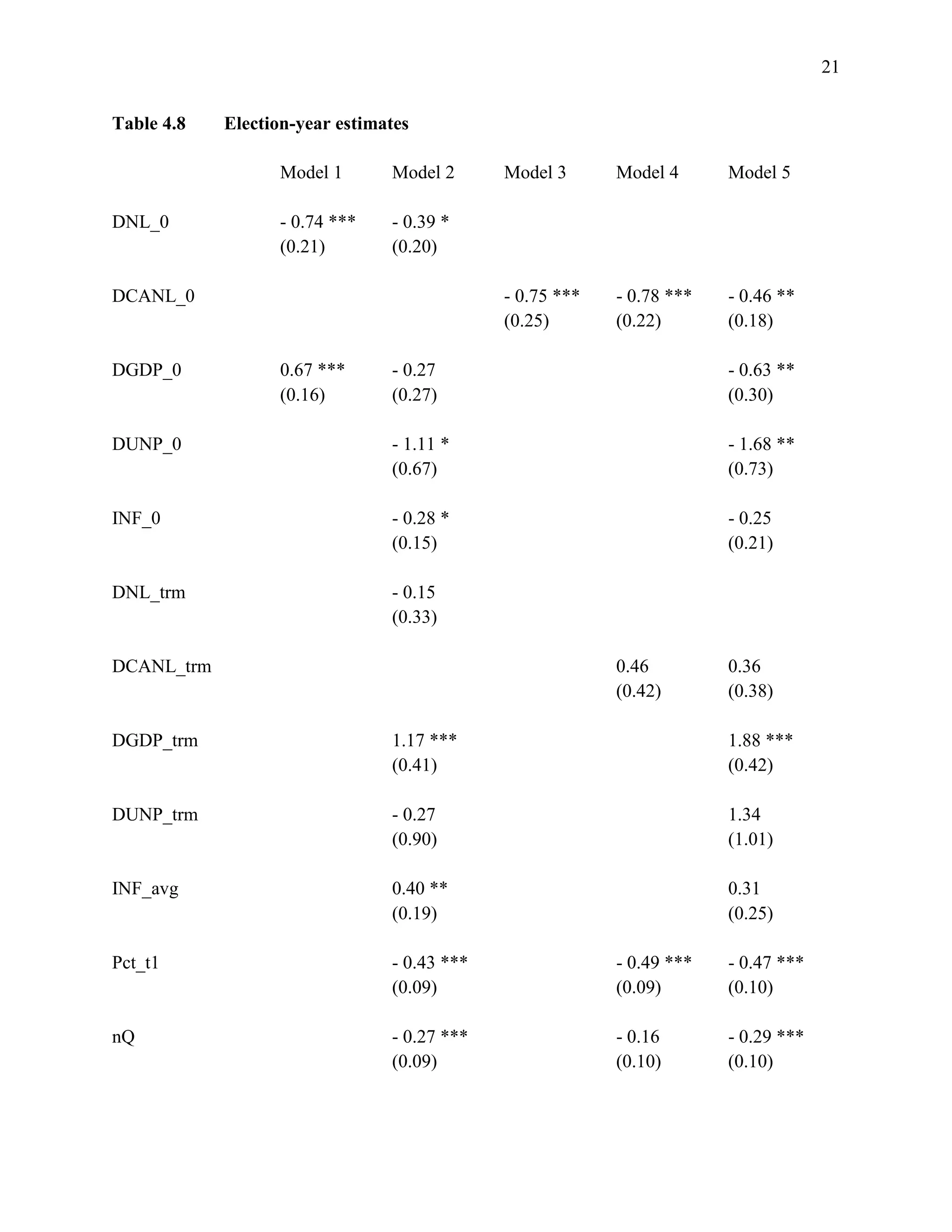
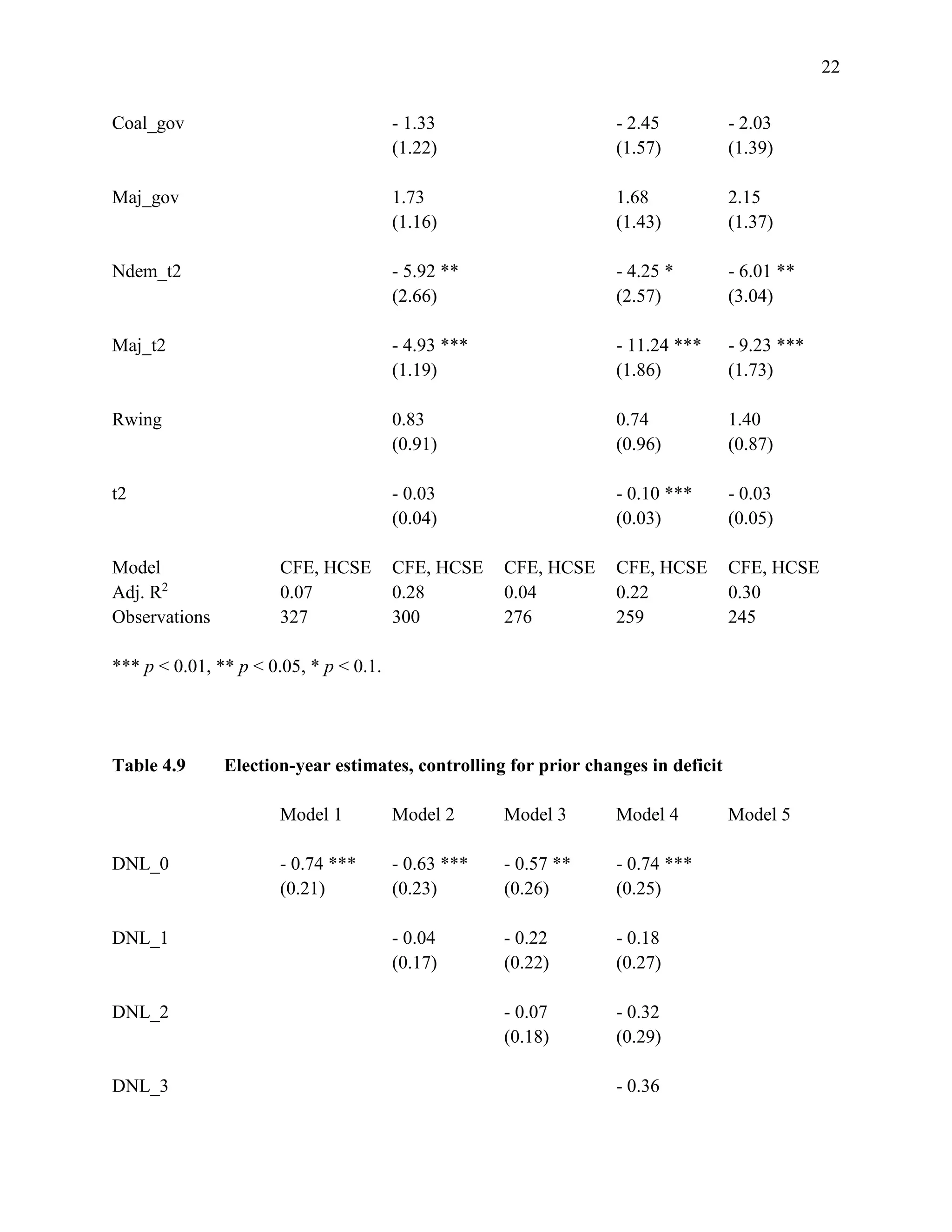
Table 4.8 presents election-year estimates of changes in general government net lending on
incumbent vote share. The results are consistent across all models: voters reward governments
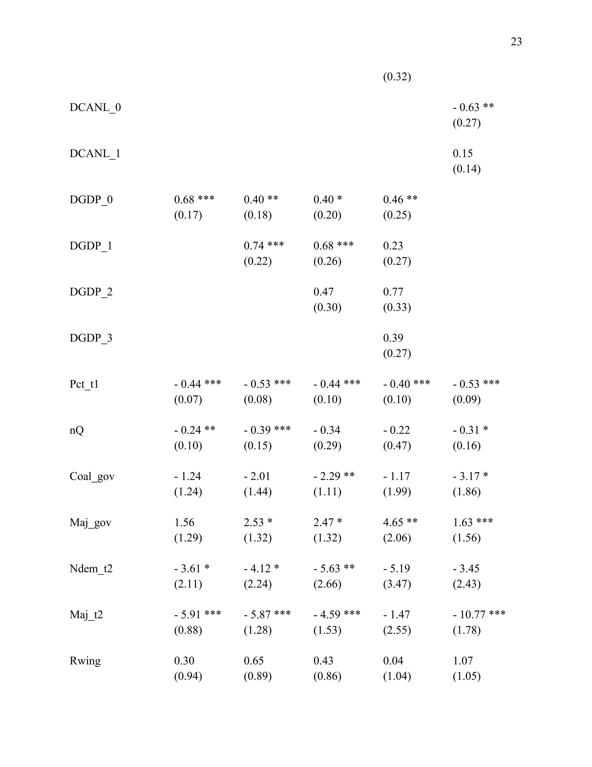
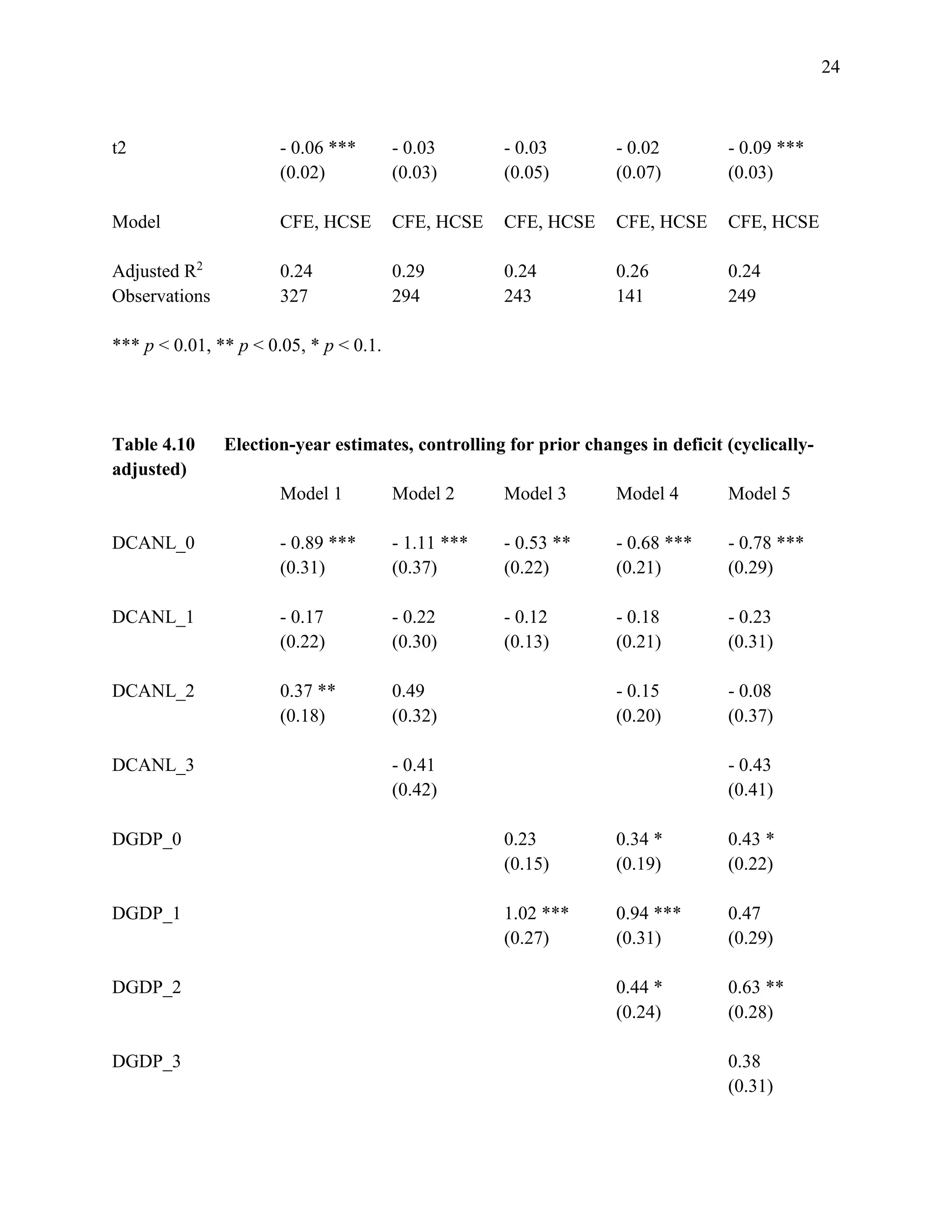
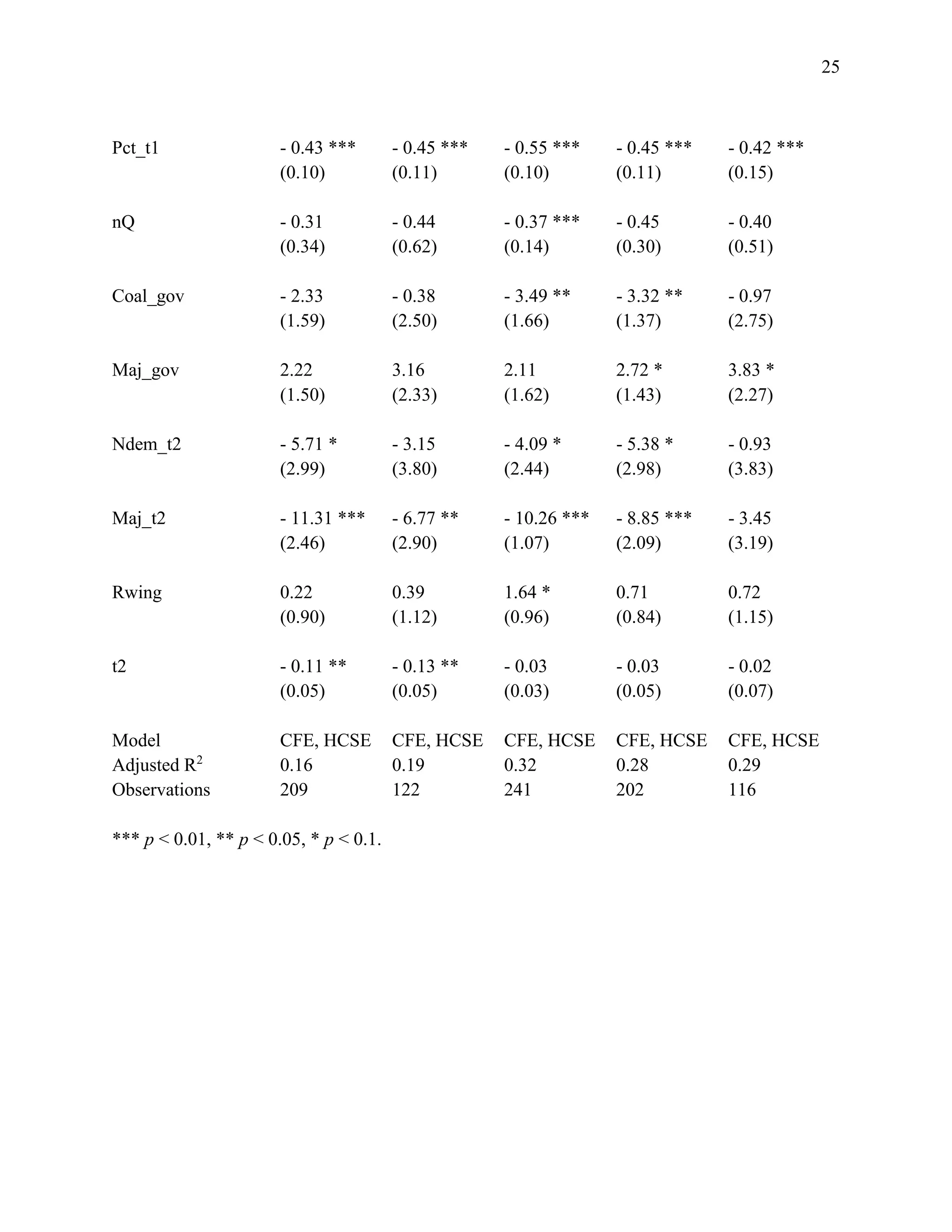
for expansionary fiscal policies in the year of election. In Tables 4.9 and 4.10, I replace DNL_trm
and DCANL_trm with variables measuring lagged changes in the fiscal deficit. Vote share
increases significantly with the election-year deficit in each model (p < 0.05), except for Table
4.10, Model 5, in which including three-year lags for the cyclically-adjusted deficit increases the
standard errors such that the estimated effect of DCANL_0 is significant only at α < 0.1.
However, including a third-year lag slightly increases the magnitude of DCANL_0.
Heterogeneous effects of changes in receipts, disbursements, and social expenditure
Alesina, Carloni, and Lecce (2013) claim that governments that reduce deficits through cuts in
government spending tend to survive longer than governments that reduce deficits through tax
increases. Although I find no evidence that voters reward governments for fiscal adjustments –
and consistently find that voters punish contractionary fiscal policies in election years – it is
possible that voters respond differently to tax versus spending measures when sanctioning
incumbents. To test for potentially heterogeneous effects of expenditure-based and revenue-
based fiscal adjustments, I examine the relationship between election-term and election-year
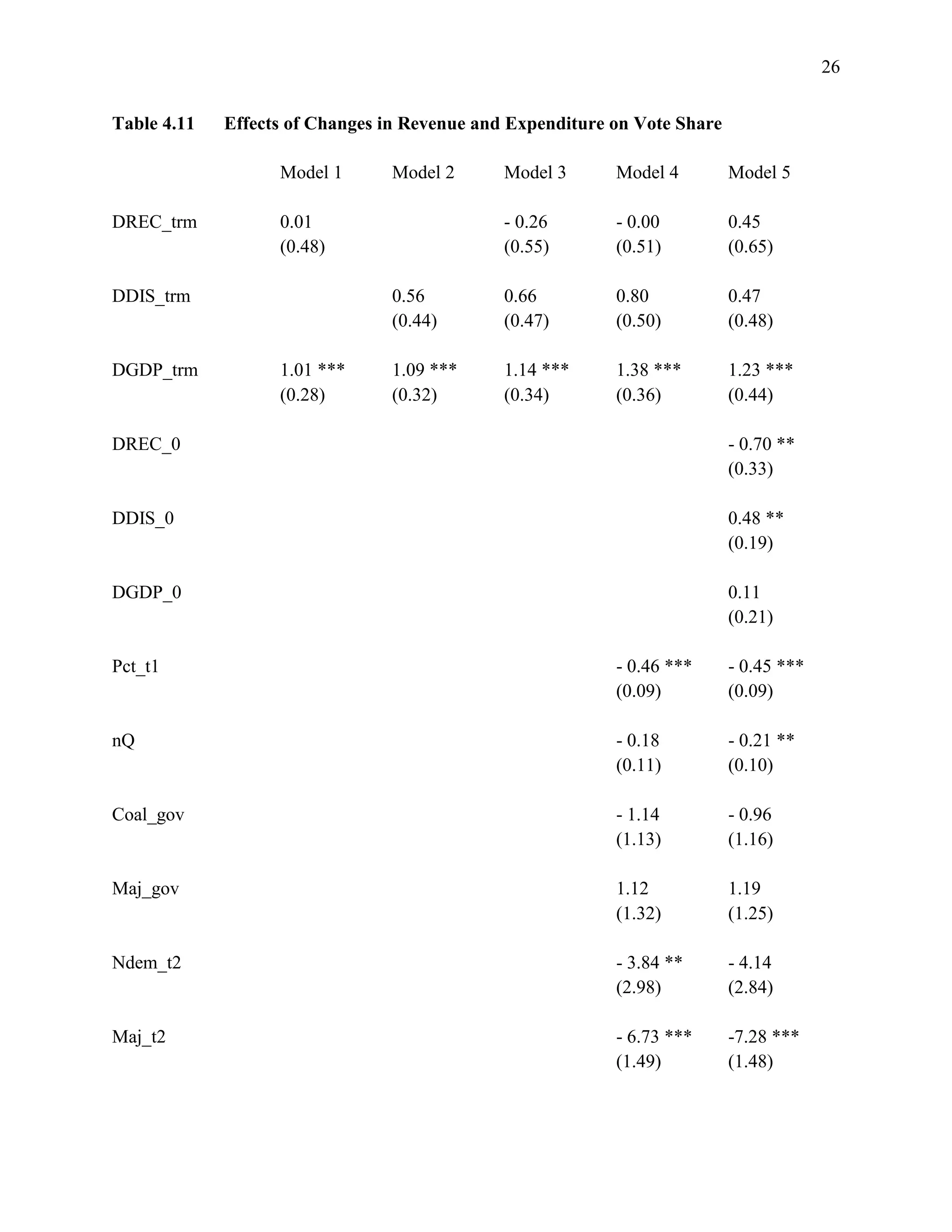
changes in expenditure and revenue (as a share of GDP) and incumbent vote share. I present the
results in Table 4.11.
[Table 4.11 here]
Table 4.11 shows no statistically significant estimated effects of term-length changes in
government receipts or disbursements on incumbent vote share. Voters do not generally oppose
higher taxes to the extent that higher taxes correspond to higher government spending over the
course of the term (Model 1). However, voters generally oppose term-length tax hikes used to
fund fiscal contractions (Model 3). Voters tend to reward governments for increasing spending,
regardless of whether the spending leads to higher taxes or fiscal expansion (Models 2-4), though
the association is not statistically significant at conventional levels.
The estimated magnitudes of term-length fiscal variables become substantially weaker once
controlling for election-year measures (Model 5). In election years, the incumbent vote share
increases with disbursement-based changes in the budget balance. Voters generally reward
(punish) tax-based fiscal expansions (contractions), but the estimated effect is not statistically
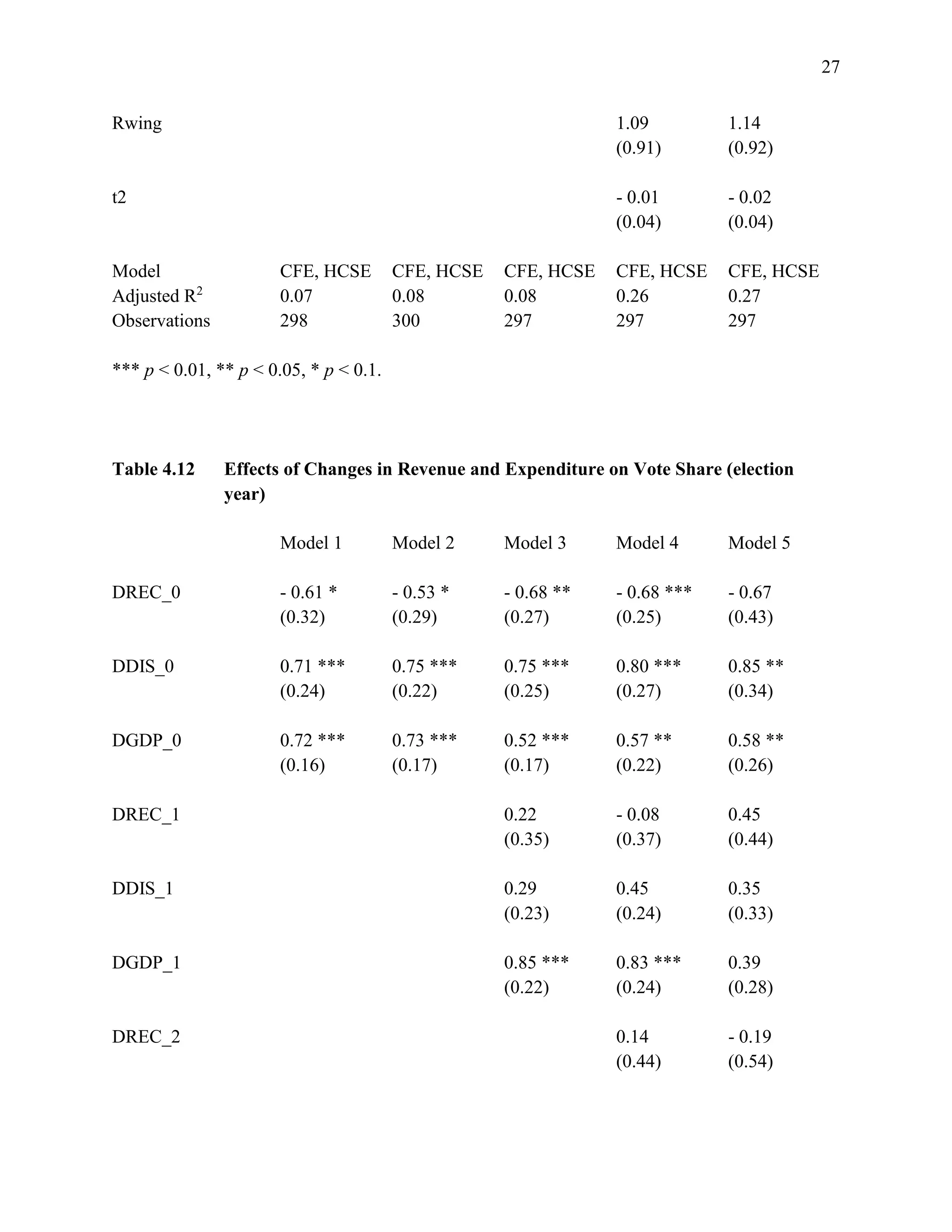
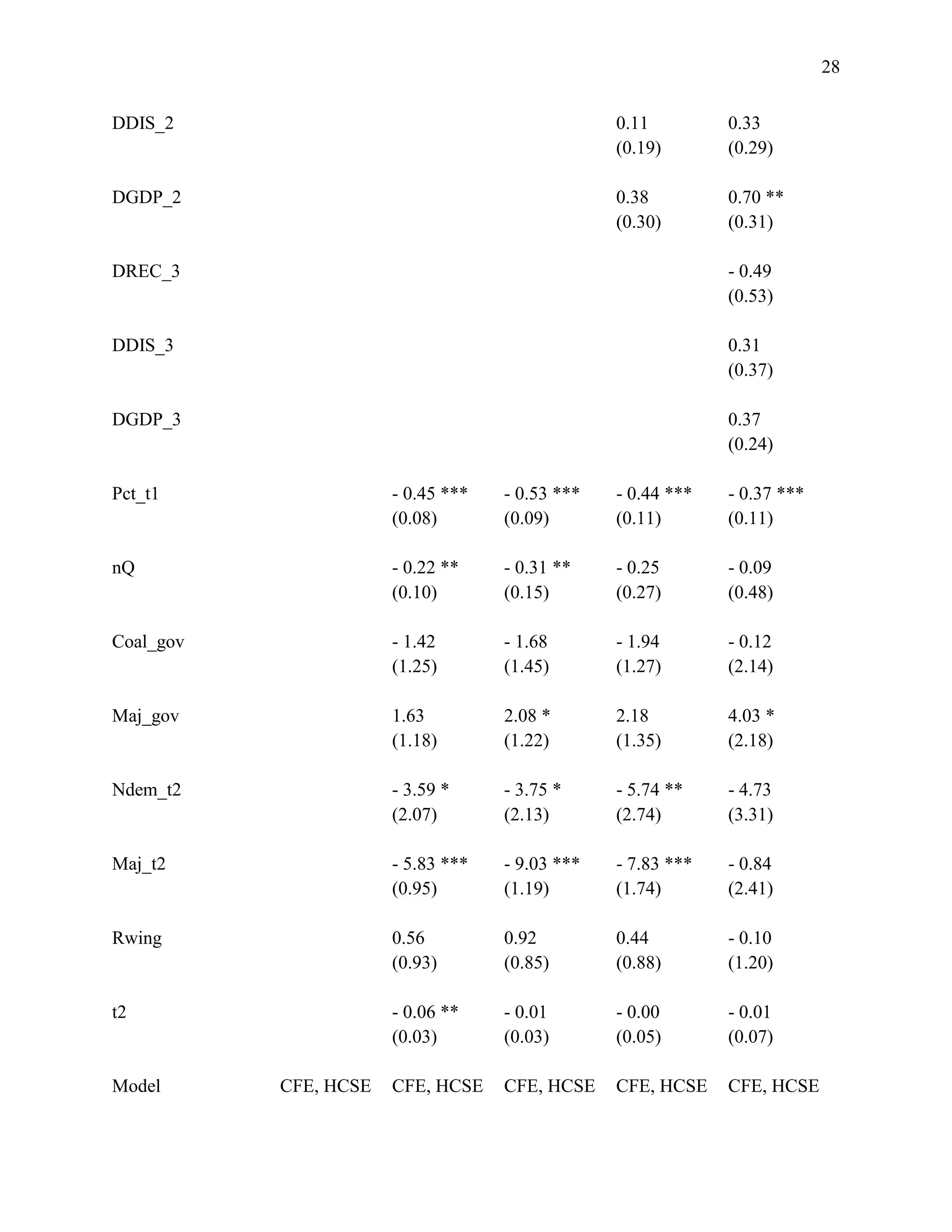
significant. Table 4.12 presents estimates of the effects of changes in election-year revenue and
expenditure on vote share, controlling for lagged changes in fiscal variables.
[Table 4.12 here]

10
Estimated election-year effects on the change in incumbent vote share remain positive and
significant for changes in disbursements and negative for changes in receipts (significant at α <
.05 in Model 3). Prior annual changes in fiscal variables have no significant effect on incumbent
vote share once controlling for election-year changes in receipts and disbursements.
Voters may plausibly evaluate changes in social (or welfare) expenditure differently than
changes in other forms of government expenditure (Pierson 1996). Yet recent research has
demonstrated no significant general effect on incumbent vote share of changes in replacement
rates for sick pay, unemployment insurance, and public pensions (Armingeon and Giger 2008;
Giger and Nelson 2010). However, as the analyses in this chapter have suggested, there is no
clear prior reason to suppose that voters sanction incumbents for term-length changes in
expenditure. Moreover, it is unclear whether voters in fact respond differently to changes in
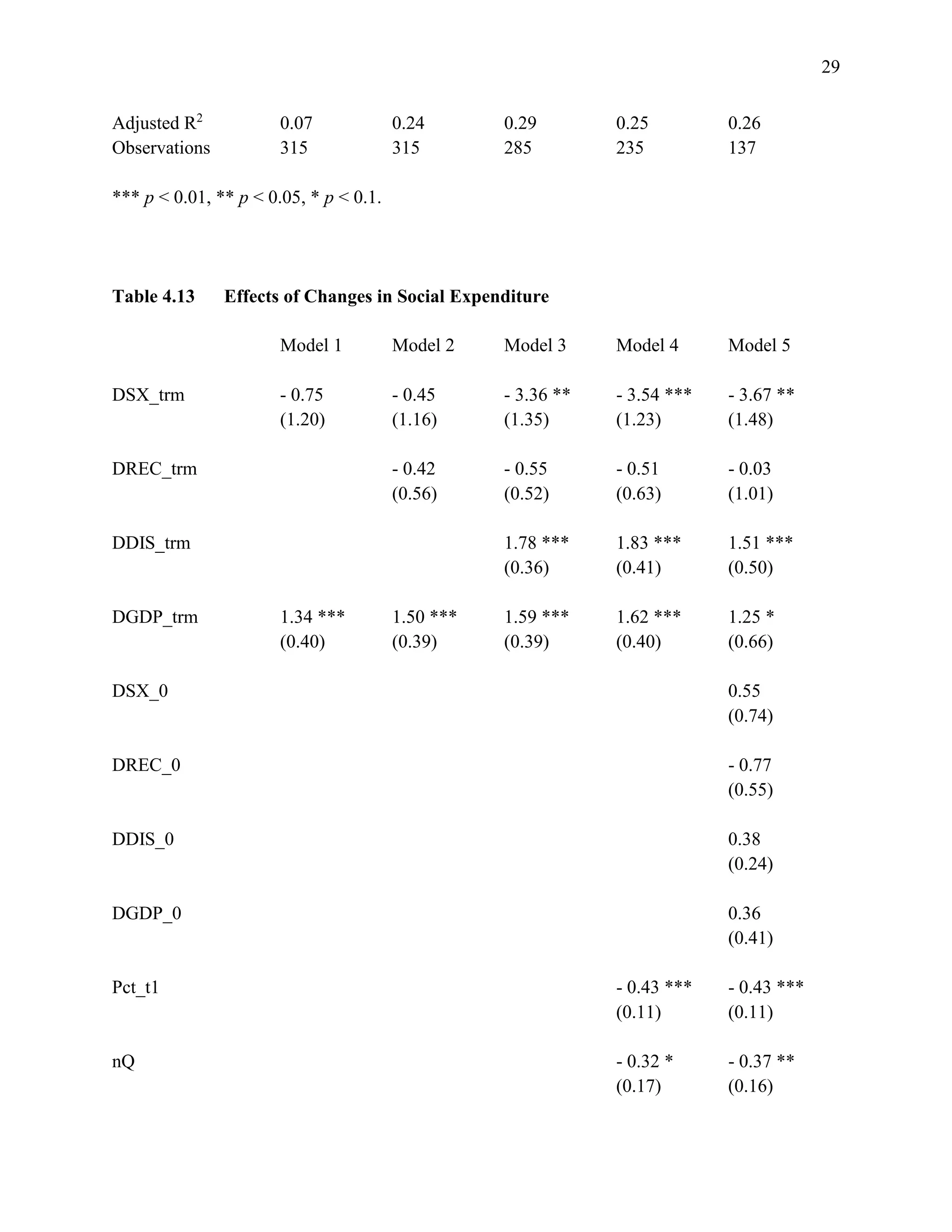
social expenditure in comparison to changes in other government disbursements. Table 4.13
examines term-length effects of changes in social expenditure. I use data from the OECD’s
(2015d) Social Expenditure Database, which includes public spending on pensions, active labor
market programs, disability and unemployment insurance, family, health, housing, and
survivors’ benefits, and “other social policy areas” (comprising 3% of social expenditure at the
OECD level).
[Table 4.13 here]
The association between changes in incumbent party vote share and term-length changes in
social expenditure is remarkably weak, regardless of whether contemporaneous changes in
government receipts are allowed to vary (Model 1) or fixed (Model 2). However, once changes
in government receipts and disbursements are both fixed, changes in social expenditure are
negatively associated with changes in incumbent vote share (p < 0.1 in Model 3; p < 0.05 in
Model 4). Voters generally reward governments for election-term expansions in non-social
expenditure, but punish governments for increasing welfare expenditure at the expense of
reductions in non-welfare government disbursements. These effects remain after controlling for
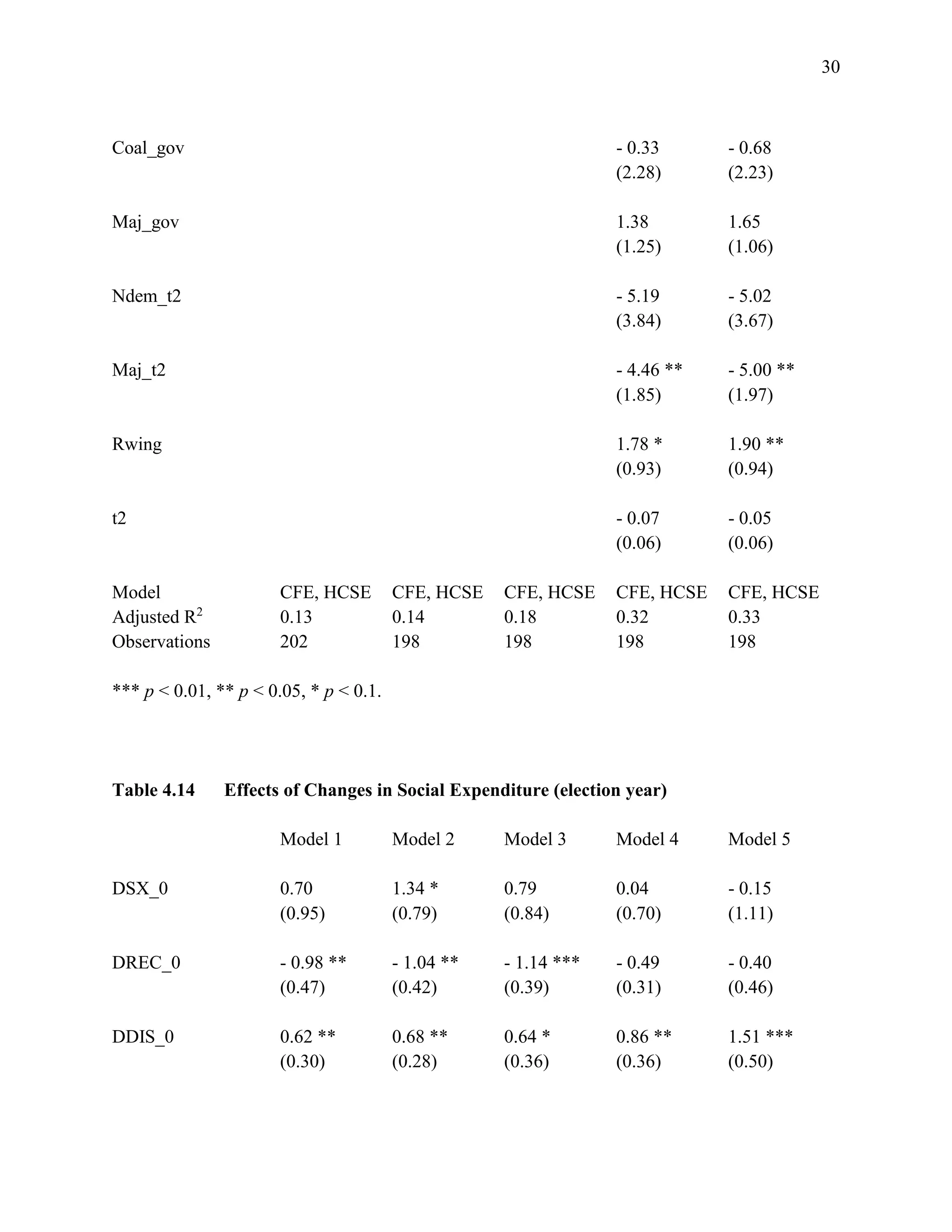
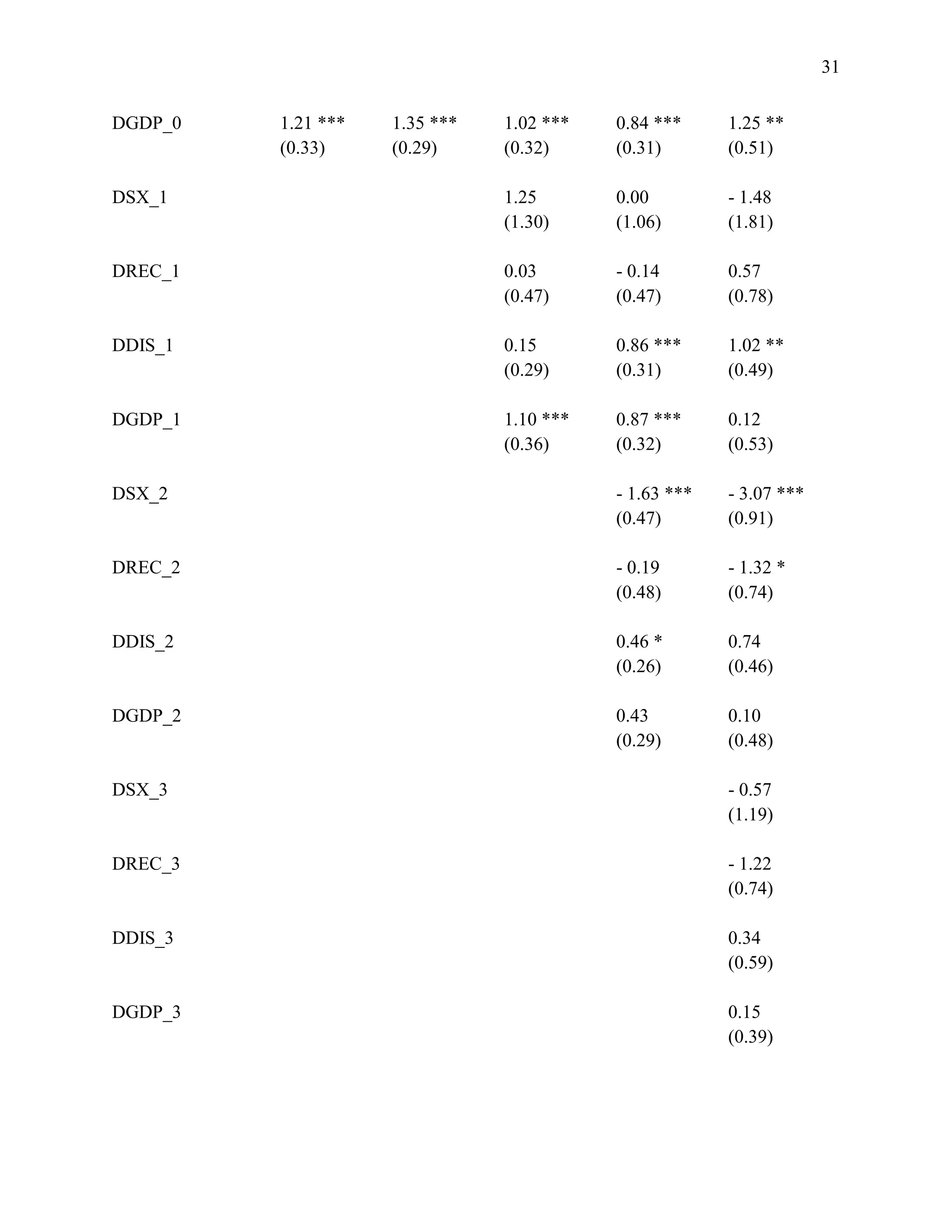
election-year changes in fiscal variables (Model 5). In contrast, incumbent vote share tends to
increase with election-year expansions in social expenditure, though the estimates are
insignificant at α < 0.05 and do not persist after controlling for two and three-year lagged
changes in social expenditure. I present these estimates in the following table.
[Table 4.14 here]
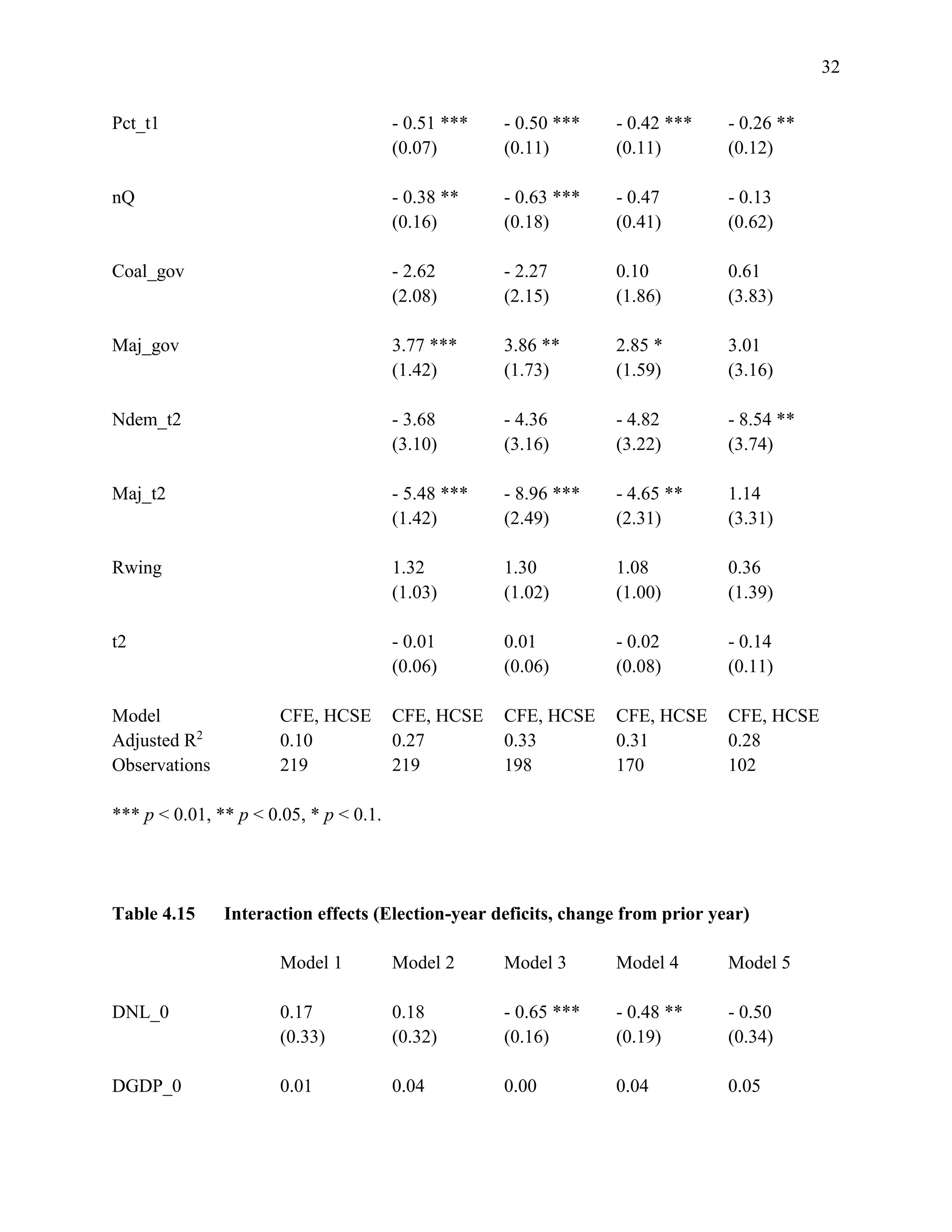
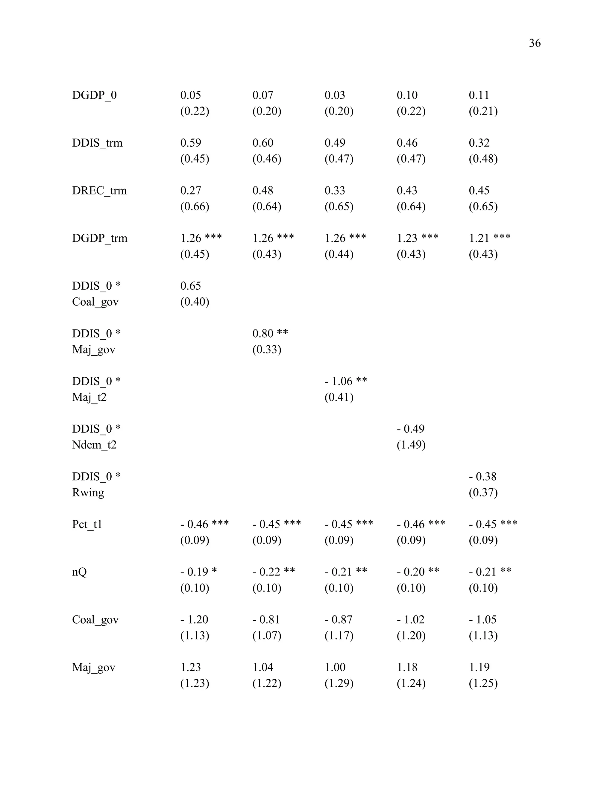
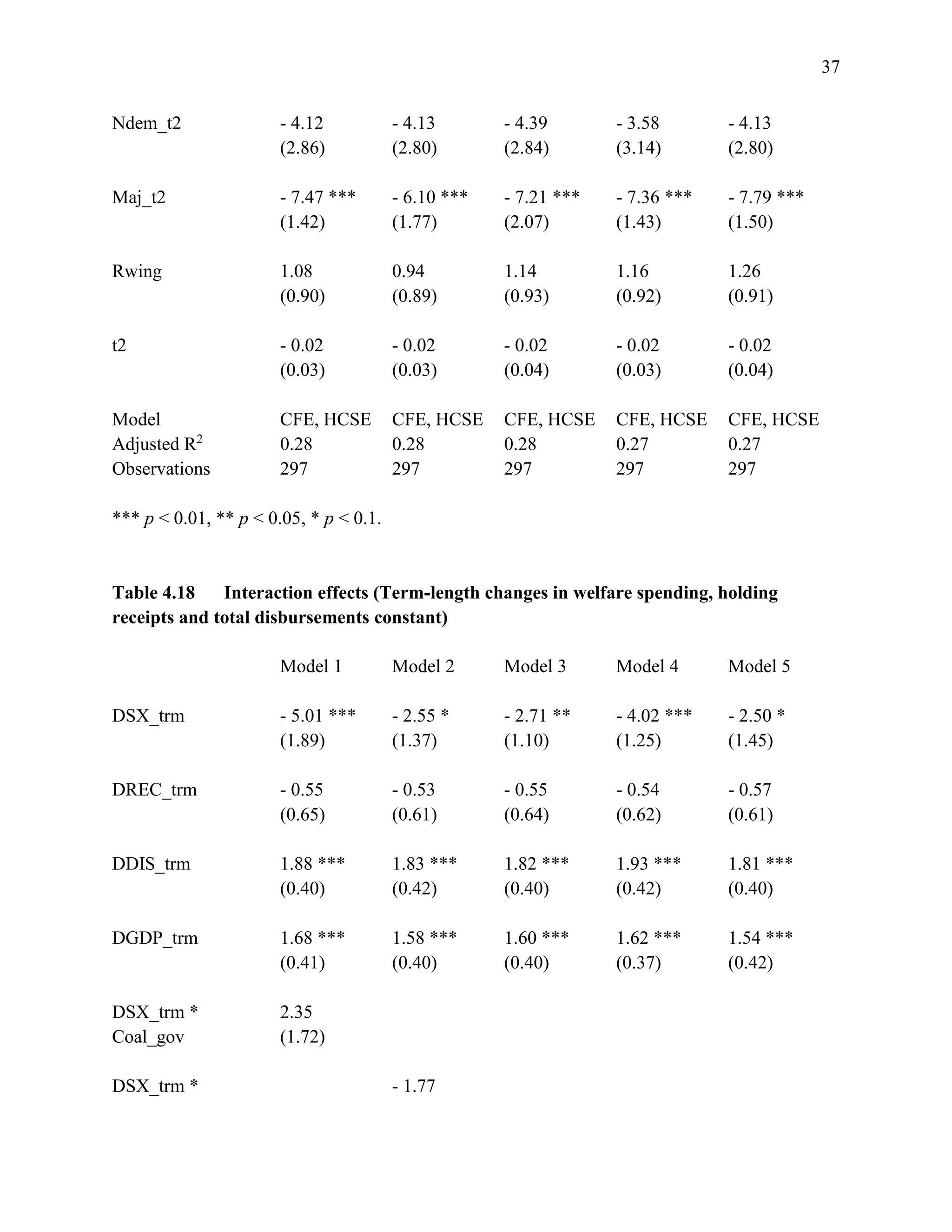
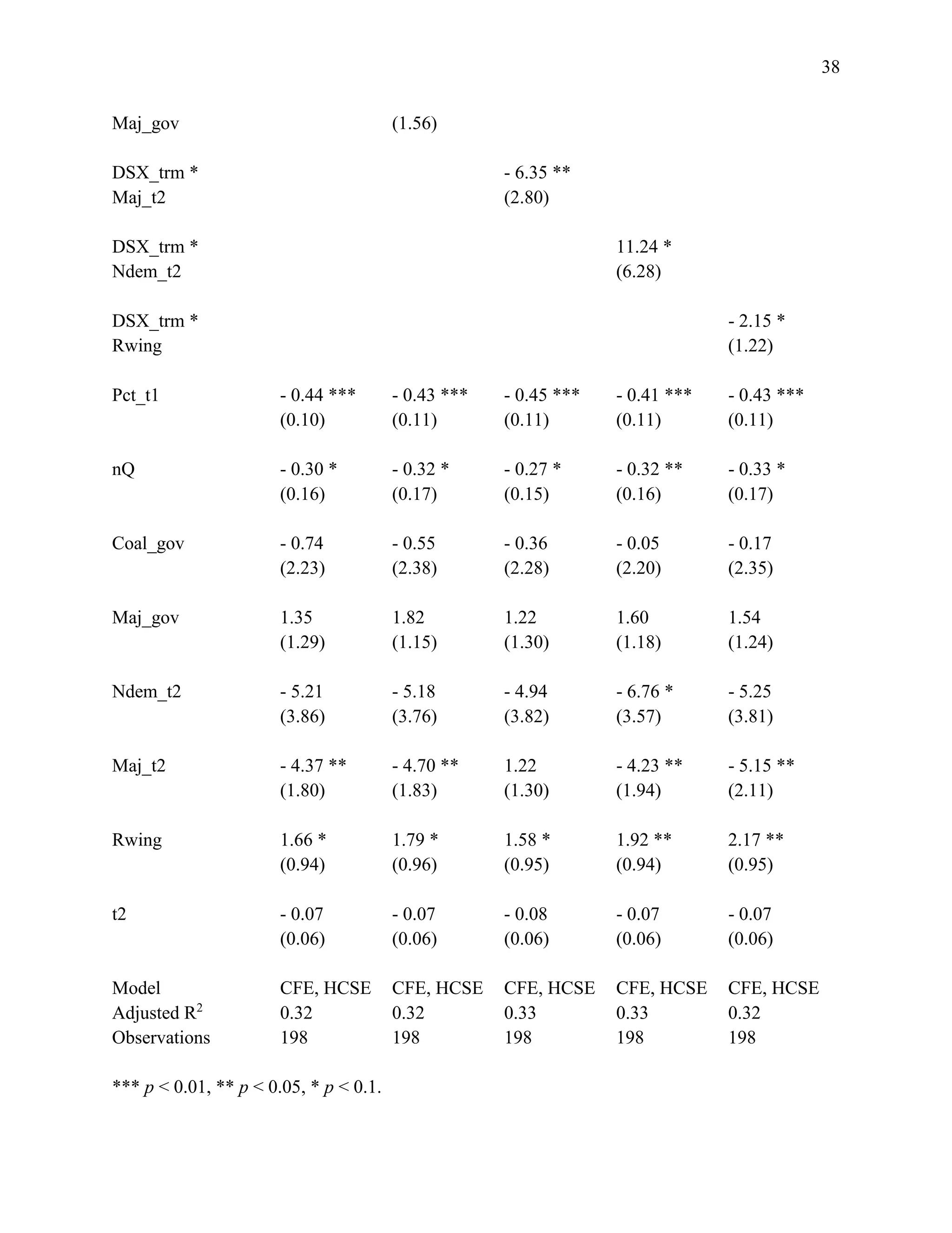
Interaction effects
The remaining models examine interaction effects between characteristics of the incumbent
government and political system and fiscal variables identified as significant determinants of

11
changes in incumbent vote share. I include four fiscal variables: change in election-year net
lending, cyclically-adjusted net lending, and disbursements (holding change in receipts constant);
and change in election-term welfare spending (holding change in receipts and disbursements
constant). I interact each fiscal variable with binary indicators of whether or not the government
facing reelection at t2 is a coalition (Coal_gov), holds a majority of seats in the lower house of
parliament (Maj_gov), is right-wing (Rwing); and whether or not the elections at t2 are one of the
first four elections held after the country’s transition to democracy (Ndem_t2), or are conducted
under majoritarian electoral rules (Maj_t2).
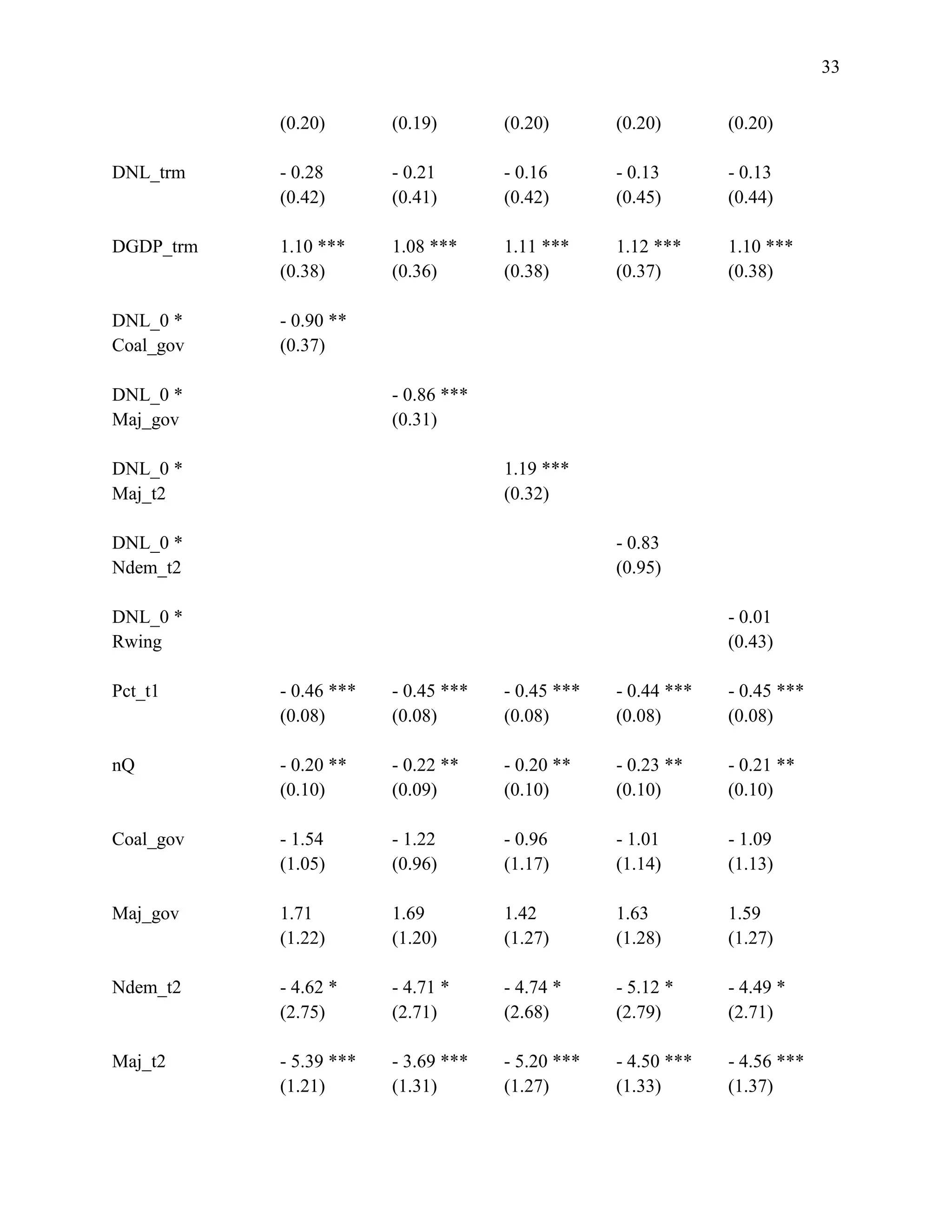
Models 1 and 2 in Tables 4.15-4.18 evaluate the interaction of each fiscal variable with
minority and coalition government indicator variables. Prior research has shown that voters are
less likely to sanction incumbent governments for changes in macroeconomic conditions in
political systems with lower “clarity of government responsibility.” When legislative and
executive power is dispersed among coalition partners, or when governments rely on the support
of opposition parties to pass legislation (including the government budget), voters may find it
more difficult to attribute credit or blame to the party of the chief executive. A related argument
suggests that governments can reduce the political costs associated with welfare retrenchment by
sharing responsibility for reforms with a range of political actors. Similarly, voters may be less
likely to reward or punish minority and coalition governments for changes in the level or
composition of revenue and expenditure. I present these estimates in the following tables.
Interestingly, voters generally punish the party of the chief executive in coalition governments –
but not in single-party administrations – for election-year reductions in the budget deficit. At the
very least, this evidence casts doubt on the applicability of the “clarity of responsibility” and
“blame sharing” hypotheses to explaining variation in the extent to which voters sanction
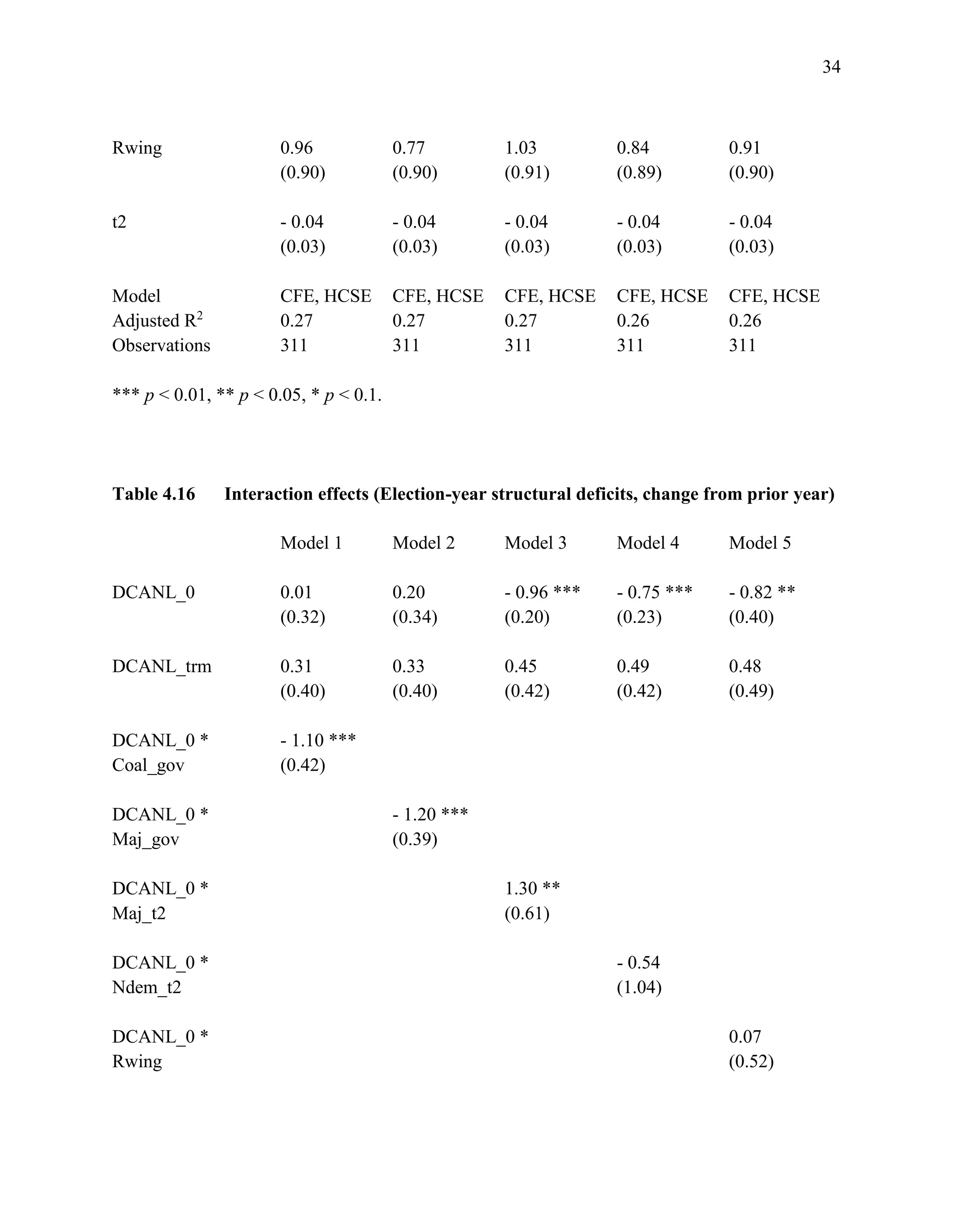
governments for fiscal adjustments. Voters do appear to punish the chief executive’s party in
coalition governments less than single-party governments for term-length changes in welfare
spending, holding other expenditure measures constant (Table 4.18). However, voters generally
reward governments for cutting welfare spending rather than non-welfare disbursements over the
course of the election cycle. Rather than helping primary coalition partners to spread the blame
for supposedly unpopular welfare cuts, sharing legislative responsibility with coalition partners
apparently inhibits the ability of such parties to claim credit for popular reforms. Unfortunately,
the standard error of the interaction term is too large for the effects to be significant at
conventional levels. The estimated effects are similar for minority governments, though also
insignificant.
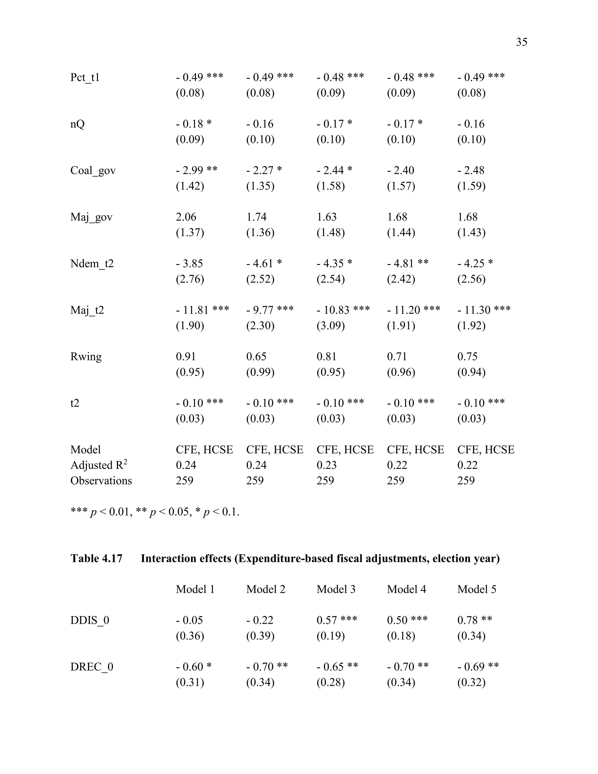
Electoral punishment for fiscal adjustments is generally confined to governments facing
reelection under proportional electoral rules (Tables 4.15-4.17, Model 3). Yet majoritarian
systems may enable governments to claim credit for election-term reductions in welfare
expenditure (Table 4.18, Model 3). Contrary to Brender and Drazen (2005; 2008), I find no

12
significant evidence that voters sanction changes in the level and composition of government
expenditure and revenue differently in new democracies (Tables 4.15-4.18, Model 4). Nor do
voters evaluate governments headed by right-wing parties differently than other administrations
(Tables 4.15-4.18, Model 5).
Conclusion
Academic and popular discussion of the political consequences of fiscal austerity suffers from a
lack of evidence-based analysis. In this chapter, I have attempted to evaluate the electoral effects
of changes in fiscal policy at the national level. The findings challenge the conclusions of prior
empirical research and the assumptions of prevailing theories of fiscal adjustment and welfare
retrenchment. Drawing from a larger number of observations than previous studies, controlling
for a wider range of potentially confounding variables, and more accurately and precisely
measuring electoral outcomes, I find no significant evidence that voters sanction incumbent
governments for term-length changes in the fiscal deficit. However, voters generally punish
governments for election-year reductions in the deficit, particularly when fiscal contractions
involve spending cuts.
Welfare programs appear no more popular than other forms of disbursements, and
governments appear to lose (gain) votes by expanding (cutting) welfare spending at the expense
(benefit) of other categories of expenditure over the course of their term in office. I also find no
evidence that electoral punishment for fiscal contractions is weaker under governments in which
the party of the chief executive shares legislative and executive power with coalition partners and
opposition parties. To the contrary, systematic electoral punishment is limited entirely to
coalition and minority governments.
Further research is necessary to identify a causal relationship between election-year fiscal
contractions (expansions) and declining (increasing) incumbent party vote share. Precise
identification of causality is inhibited by the fact that observed discretionary changes in fiscal
variables are not randomly assigned. A number of variables outside the researcher’s control
affect the degree to which governments implement fiscal expansions or contractions.3
Although
the evidence presented in this chapter indicates that voters tend to reward looser fiscal policy in
election years, the relationship between fiscal and electoral outcomes varies considerably across
countries and time. While this chapter describes the general relationship between fiscal and
electoral outcomes, understanding why voters reward or punish governments in particular cases
requires more detailed contextual analysis.
3
See Chapter Two on the political causes of budget deficits.

13
Table 4.1 Sample of countries
Number of observations 327
Number of countries 30
Period (Election Years) 1944-2015
Country (number of observations) / Election years
Australia (21) 1961 – 2013
Austria (16) 1962 – 2013
Belgium (16) 1961 – 2014
Canada (17) 1962 – 2011
Czech Republic (5) 1998 – 2013
Denmark (19) 1973 – 2011
Estonia (3) 2003 – 2011
Finland (14) 1962 – 2011
France (11) 1967 – 2012
Germany (15) 1961 – 2013
Greece (13) 1961 – 2009
Hungary (5) 1998 – 2014
Iceland (15) 1983 – 2013
Ireland (14) 1981 – 2011
Israel (7) 1999 – 2013
Italy (11) 1963 – 2008
Japan (17) 1963 – 2014
Korea (2) 2007 – 2012
Luxembourg (11) 1989 – 2013
Netherlands (16) 1971 – 2012
New Zealand (17) 1987 – 2014
Norway (14) 1965 – 2013
Poland (5) 1997 – 2011
Portugal (11) 1979 – 2011
Slovakia (6) 1998 – 2012
Slovenia (5) 2000 – 2014
Spain (10) 1979 – 2011
Sweden (16) 1964 – 2014
United Kingdom (13) 1964 – 2010
United States (17) 1964 – 2012

14
Table 4.2 Descriptive Statistics
Political variables (binary, N = 327)
Variable Mean Std. Dev. 0 1 .
Coal_gov 0.54 0.50 150 177
Maj_gov 0.68 0.47 105 222
Ndem_t2 0.08 0.28 300 27
Rwing 0.56 0.50 145 182
Maj_t2 0.29 0.46 231 96
Reelect 0.58 0.49 136 191
Other variables (N = 327)
Variable Mean Std. Dev. Min Max
DPct -2.80 7.45 -29.73 20.70
Pct_t1 37.16 10.41 8.59 61.05
nQ 12.97 4.12 1 20
Pct_t2 34.36 11.10 2.97 61.05
t1 1987 15.04 1957 2012
t2 1991 15.18 1961 2014
q2 2.65 1.10 1 4
Receipts
Variable Mean Std. Dev. Min Max N
DREC_0 0.10 1.20 -4.20 6.73 316
DREC_1 0.13 1.07 -3.39 2.96 285
DREC_2 0.19 1.18 -2.90 6.72 235
DREC_3 0.28 1.22 -3.02 4.07 138
DREC_trm 0.15 0.75 -3.55 2.48 300
Disbursements
DDIS_0 0.18 2.23 -20.17 8.79 315
DDIS_1 0.30 2.19 -7.62 18.47 285

15
DDIS_2 0.20 2.12 -6.75 7.77 236
DDIS_3 0.02 1.86 -6.48 6.70 140
DDIS_trm 0.19 1.24 -10.43 3.76 302
Net Lending
DNL_0 -0.07 2.16 -8.36 19.78 302
DNL_1 -0.13 2.26 -18.48 5.62 296
DNL_2 0.00 2.16 -8.37 6.86 262
DNL_3 0.25 2.03 -7.26 5.39 245
DNL_trm -0.02 1.24 -7.31 9.95 314
BALCH_trm 0.03 2.55 -19.72 6.89 295
BALCH_termPey -0.16 2.26 -16.33 5.63 295
BTxDS -2.62 11.38 -88.72 30.74 288
DNL0xDS -1.22 14.76 -149.30 58.15 313
Cyclically-adjusted net lending
DCANL_0 -0.15 2.04 -5.94 17.75 268
DCANL_1 -0.26 2.20 -18.97 4.56 241
DCANL_2 0.20 1.83 -6.47 6.62 202
DCANL_3 0.18 1.81 -7.04 4.72 113
DCANL_trm - 0.03 1.14 -4.06 8.79 252
Social Expenditure
DSX_0 0.25 0.90 -2.76 5.05 221
DSX_1 0.15 0.73 -2.14 2.84 203
DSX_2 0.24 1.04 -2.13 4.31 175
DSX_3 0.17 0.94 -2.42 4.08 103
DSX_trm 0.22 0.52 -1.36 1.60 202

16
GDP (annual)
DGDP_0 3.16 2.80 -5.92 13.06 327
DGDP_1 3.01 2.57 -6.55 11.91 298
DGDP_2 2.81 2.90 -14.74 11.85 248
DGDP_3 3.25 2.73 -5.48 11.19 146
DGDP_trm 3.14 2.20 -2.61 12.64 317
DGDPPC_0 2.54 2.76 -7.07 11.97 317
DGDPPC_trm 2.50 2.15 -3.21 11.18 308
DDGDP_trm -0.22 3.40 -14.87 14.33 313
Inflation
INF_0 5.34 6.99 -5.21 77.31 323
INF_1 5.70 6.36 -1.85 53.65 321
INF_2 5.66 6.39 -3.92 49.19 292
INF_3 5.49 6.37 -2.48 52.48 243
INF_avg 5.69 6.43 -1.78 60.05 312
Unemployment
DUNP_0 0.05 1.04 -4.42 4.31 322
DUNP_1 0.09 0.93 -3.91 3.65 302
DUNP_2 0.27 1.51 -2.58 13.33 255
DUNP_3 -0.08 1.00 -3.32 5.06 151
DUNP_trm 0.09 0.79 -4.07 3.39 322

17
Table 4.3 Replication of Brender-Drazen
Model 1 Model 2 Model 3
Dependent variable Reelect Reelect DPct
BALCH_trm 0.04 (0.06) 0.01 (0.08) - 0.01 (0.18)
DNL_0 - 0.04 (0.06) - 0.04 (0.09) - 0.43 (0.21) **
DGDPPC_trm 0.21 (0.07) *** 0.32 (0.10) *** 1.31 (0.24) ***
Ndem_t2 - 0.60 (0.51) 0.14 (0.79) - 3.70 (2.47)
Maj_t2 0.37 (0.28) - 0.31 (1.87) - 3.85 (3.11) ***
Pct_t1 - 0.47 (0.07) ***
Model Logit Logit, CFE, HCSE CFE, HCSE
R2
0.05 0.16
Adjusted R2
0.25
Observations 281 281 281
Standard errors in parentheses. *** p < 0.01, ** p < 0.05, * p < 0.1.
Table 4.4 Replication of Brender-Drazen (continued)
Model 4 Model 5 Model 6 Model 7
Dependent variable Reelect DPct Reelect DPct
BALCH_trm 0.05 (0.06) - 0.01 (0.18) 0.04 (0.06) - 0.01 (0.19)
DNL_0 - 0.08 (0.07) - 0.43 (0.24) * - 0.06 (0.07) - 0.37 (0.24)
DGDPPC_trm 0.13 (0.10) 1.31 (0.34) *** 0.20 (0.08) *** 1.35 (0.25) ***
DGDPPC_0 0.09 (0.08) - 0.00 (0.24)
GDPD_trend_ey 0.01 (0.01) - 0.02 (0.03)
Ndem_t2 - 0.61 (0.51) - 3.70 (2.48) - 0.59 (0.51) - 3.79 (2.47)
Maj_t2 0.38 (0.28) - 3.85 (3.13) *** 0.37 (0.28) - 3.79 (3.16)
Pct_t1 - 0.47 (0.07) *** - 0.48 (0.08) ***
Model Logit, HCSE CFE, HCSE Logit, HCSE CFE, HCSE
R2
0.05 0.05
Adjusted R2
0.25 0.25

18
Observations 281 281 281 281
Table 4.5 Replication of Brender-Drazen (continued)
Dependent variable Reelect DPct Reelect DPct
BALCH_trm 0.03 (0.06) - 0.08 (0.18)
DNL_0 - 0.07 (0.07) - 0.43 (0.17) ** - 0.06 (0.07) - 0.50 (0.18) **
DGDPPC_trm 0.21 (0.07) *** 1.29 (0.22) *** 0.23 (0.08) *** 1.35 (0.26) ***
BALCH_termPey 0.06 (0.06) 0.02 (0.19)
BTxDS - 0.00 (0.01) - 0.01 (0.03)
DNL0xDS - 0.01 (0.01) - 0.04 (0.02)
Ndem_t2 - 0.60 (0.50) * - 3.69 (2.44) - 0.53 (0.54) - 3.71 (2.73) **
Maj_t2 0.36 (0.28) - 3.93 (3.13) 0.33 (0.29) - 3.84 (2.96)
Pct_t1 - 0.47 (0.07) *** - 0.48 (0.07) ***
Model Logit, HCSE CFE, HCSE Logit, HCSE CFE, HCSE
R2
0.05 0.05
Adjusted R2
0.25 0.25
Table 4.6 Replication of Nyman
Dependent variable Reelect DPct DPct DPct
Structural budget balance - 0.02 - 0.56
(DCANL_trm) (0.17) (0.50)

19
Non-adjusted budget balance 0.03 - 0.44
(DNL_trm) (0.51) (0.47)
Change in unemployment rate - 0.35 - 1.82 ** - 1.08
(DUNP_trm) (0.22) (0.76) (0.82)
Change in GDP growth - 0.00 0.02 0.05
(DDGDP_trm) (0.04) (0.13) (0.12)
Average GDP growth 0.13 0.53 ** 0.86 ***
(DGDP_trm) (0.11) (0.22) (0.27)
Right-wing party 0.48 0.50 0.83 ** 1.80 **
(Rwing) (0.28) (0.62) (0.69) (0.75)
R2
(1) / Adjusted R2
(2-4) 0.04 0.00 0.08 0.11
Model Logit, HCSE OLS, HCSE OLS, HCSE OLS, HCSE
Country fixed effects included. Standard errors in parentheses.
*** p < 0.01, ** p < 0.05, * p < 0.1.
Table 4.7 Term-length estimates
Model 1 Model 2 Model 3 Model 4 Model 5
DNL_trm - 0.44 - 0.26
(0.45) (0.34)
DCANL_trm - 0.48 - 0.06 0.14
(0.50) (0.50) (0.41)
DGDP_trm 1.01 *** 0.82 ** 1.24 ***
(0.31) (0.29) (0.28)
DUNP_trm - 1.38 ** - 0.44
(0.56) (0.62)

20
INF_avg 0.11 0.07
(0.07) (0.06)
Pct_t1 - 0.44 *** - 0.50 *** - 0.47 ***
(0.08) (0.08) (0.09)
nQ - 0.22 ** - 0.09 - 0.23 **
(0.09) (0.11) (0.11)
Coal_gov - 1.46 - 2.28 - 2.06
(1.24) (1.54) (1.39)
Maj_gov 1.57 1.34 2.06
(1.22) (1.53) (1.39)
Ndem_t2 - 5.20 * - 3.94 - 5.61 *
(2.75) (2.84) (3.19)
Maj_t2 - 4.77 *** - 10.45 *** - 8.10 ***
(1.12) (2.24) (2.13)
Rwing 0.72 0.66 1.24
(0.93) (0.98) (0.93)
t2 - 0.04 - 0.12 *** - 0.04
(0.04) (0.03) (0.05)
Model CFE, HCSE CFE, HCSE CFE, HCSE CFE, HCSE CFE, HCSE
Adjusted R2
0.07 0.27 0.00 0.19 0.28
Observations 311 301 259 259 246
*** p < 0.01, ** p < 0.05, * p < 0.1.

21
Table 4.8 Election-year estimates
DNL_0 - 0.74 *** - 0.39 *
(0.21) (0.20)
DCANL_0 - 0.75 *** - 0.78 *** - 0.46 **
(0.25) (0.22) (0.18)
DGDP_0 0.67 *** - 0.27 - 0.63 **
(0.16) (0.27) (0.30)
DUNP_0 - 1.11 * - 1.68 **
(0.67) (0.73)
INF_0 - 0.28 * - 0.25
(0.15) (0.21)
DNL_trm - 0.15
(0.33)
DCANL_trm 0.46 0.36
(0.42) (0.38)
DGDP_trm 1.17 *** 1.88 ***
(0.41) (0.42)
DUNP_trm - 0.27 1.34
(0.90) (1.01)
INF_avg 0.40 ** 0.31
(0.19) (0.25)
Pct_t1 - 0.43 *** - 0.49 *** - 0.47 ***
(0.09) (0.09) (0.10)
nQ - 0.27 *** - 0.16 - 0.29 ***
(0.09) (0.10) (0.10)

22
Coal_gov - 1.33 - 2.45 - 2.03
(1.22) (1.57) (1.39)
Maj_gov 1.73 1.68 2.15
(1.16) (1.43) (1.37)
Ndem_t2 - 5.92 ** - 4.25 * - 6.01 **
(2.66) (2.57) (3.04)
Maj_t2 - 4.93 *** - 11.24 *** - 9.23 ***
(1.19) (1.86) (1.73)
Rwing 0.83 0.74 1.40
(0.91) (0.96) (0.87)
t2 - 0.03 - 0.10 *** - 0.03
(0.04) (0.03) (0.05)
Adj. R2
0.07 0.28 0.04 0.22 0.30
Observations 327 300 276 259 245
*** p < 0.01, ** p < 0.05, * p < 0.1.
Table 4.9 Election-year estimates, controlling for prior changes in deficit
DNL_0 - 0.74 *** - 0.63 *** - 0.57 ** - 0.74 ***
(0.21) (0.23) (0.26) (0.25)
DNL_1 - 0.04 - 0.22 - 0.18
(0.17) (0.22) (0.27)
DNL_2 - 0.07 - 0.32
(0.18) (0.29)
DNL_3 - 0.36

23
(0.32)
DCANL_0 - 0.63 **
(0.27)
DCANL_1 0.15
(0.14)
DGDP_0 0.68 *** 0.40 ** 0.40 * 0.46 **
(0.17) (0.18) (0.20) (0.25)
DGDP_1 0.74 *** 0.68 *** 0.23
(0.22) (0.26) (0.27)
DGDP_2 0.47 0.77
(0.30) (0.33)
DGDP_3 0.39
(0.27)
Pct_t1 - 0.44 *** - 0.53 *** - 0.44 *** - 0.40 *** - 0.53 ***
(0.07) (0.08) (0.10) (0.10) (0.09)
nQ - 0.24 ** - 0.39 *** - 0.34 - 0.22 - 0.31 *
(0.10) (0.15) (0.29) (0.47) (0.16)
Coal_gov - 1.24 - 2.01 - 2.29 ** - 1.17 - 3.17 *
(1.24) (1.44) (1.11) (1.99) (1.86)
Maj_gov 1.56 2.53 * 2.47 * 4.65 ** 1.63 ***
(1.29) (1.32) (1.32) (2.06) (1.56)
Ndem_t2 - 3.61 * - 4.12 * - 5.63 ** - 5.19 - 3.45
(2.11) (2.24) (2.66) (3.47) (2.43)
Maj_t2 - 5.91 *** - 5.87 *** - 4.59 *** - 1.47 - 10.77 ***
(0.88) (1.28) (1.53) (2.55) (1.78)
Rwing 0.30 0.65 0.43 0.04 1.07
(0.94) (0.89) (0.86) (1.04) (1.05)

24
t2 - 0.06 *** - 0.03 - 0.03 - 0.02 - 0.09 ***
(0.02) (0.03) (0.05) (0.07) (0.03)
Adjusted R2
0.24 0.29 0.24 0.26 0.24
Observations 327 294 243 141 249
*** p < 0.01, ** p < 0.05, * p < 0.1.
Table 4.10 Election-year estimates, controlling for prior changes in deficit (cyclically-
adjusted)
DCANL_0 - 0.89 *** - 1.11 *** - 0.53 ** - 0.68 *** - 0.78 ***
(0.31) (0.37) (0.22) (0.21) (0.29)
DCANL_1 - 0.17 - 0.22 - 0.12 - 0.18 - 0.23
(0.22) (0.30) (0.13) (0.21) (0.31)
DCANL_2 0.37 ** 0.49 - 0.15 - 0.08
(0.18) (0.32) (0.20) (0.37)
DCANL_3 - 0.41 - 0.43
(0.42) (0.41)
DGDP_0 0.23 0.34 * 0.43 *
(0.15) (0.19) (0.22)
DGDP_1 1.02 *** 0.94 *** 0.47
(0.27) (0.31) (0.29)
DGDP_2 0.44 * 0.63 **
(0.24) (0.28)
DGDP_3 0.38
(0.31)

25
Pct_t1 - 0.43 *** - 0.45 *** - 0.55 *** - 0.45 *** - 0.42 ***
(0.10) (0.11) (0.10) (0.11) (0.15)
nQ - 0.31 - 0.44 - 0.37 *** - 0.45 - 0.40
(0.34) (0.62) (0.14) (0.30) (0.51)
Coal_gov - 2.33 - 0.38 - 3.49 ** - 3.32 ** - 0.97
(1.59) (2.50) (1.66) (1.37) (2.75)
Maj_gov 2.22 3.16 2.11 2.72 * 3.83 *
(1.50) (2.33) (1.62) (1.43) (2.27)
Ndem_t2 - 5.71 * - 3.15 - 4.09 * - 5.38 * - 0.93
(2.99) (3.80) (2.44) (2.98) (3.83)
Maj_t2 - 11.31 *** - 6.77 ** - 10.26 *** - 8.85 *** - 3.45
(2.46) (2.90) (1.07) (2.09) (3.19)
Rwing 0.22 0.39 1.64 * 0.71 0.72
(0.90) (1.12) (0.96) (0.84) (1.15)
t2 - 0.11 ** - 0.13 ** - 0.03 - 0.03 - 0.02
(0.05) (0.05) (0.03) (0.05) (0.07)
Adjusted R2
0.16 0.19 0.32 0.28 0.29
Observations 209 122 241 202 116
*** p < 0.01, ** p < 0.05, * p < 0.1.

26
Table 4.11 Effects of Changes in Revenue and Expenditure on Vote Share
DREC_trm 0.01 - 0.26 - 0.00 0.45
(0.48) (0.55) (0.51) (0.65)
DDIS_trm 0.56 0.66 0.80 0.47
(0.44) (0.47) (0.50) (0.48)
DGDP_trm 1.01 *** 1.09 *** 1.14 *** 1.38 *** 1.23 ***
(0.28) (0.32) (0.34) (0.36) (0.44)
DREC_0 - 0.70 **
(0.33)
DDIS_0 0.48 **
(0.19)
DGDP_0 0.11
(0.21)
Pct_t1 - 0.46 *** - 0.45 ***
(0.09) (0.09)
nQ - 0.18 - 0.21 **
(0.11) (0.10)
Coal_gov - 1.14 - 0.96
(1.13) (1.16)
Maj_gov 1.12 1.19
(1.32) (1.25)
Ndem_t2 - 3.84 ** - 4.14
(2.98) (2.84)
Maj_t2 - 6.73 *** -7.28 ***
(1.49) (1.48)

27
Rwing 1.09 1.14
(0.91) (0.92)
t2 - 0.01 - 0.02
(0.04) (0.04)
Adjusted R2
0.07 0.08 0.08 0.26 0.27
Observations 298 300 297 297 297
*** p < 0.01, ** p < 0.05, * p < 0.1.
Table 4.12 Effects of Changes in Revenue and Expenditure on Vote Share (election
year)
DREC_0 - 0.61 * - 0.53 * - 0.68 ** - 0.68 *** - 0.67
(0.32) (0.29) (0.27) (0.25) (0.43)
DDIS_0 0.71 *** 0.75 *** 0.75 *** 0.80 *** 0.85 **
(0.24) (0.22) (0.25) (0.27) (0.34)
DGDP_0 0.72 *** 0.73 *** 0.52 *** 0.57 ** 0.58 **
(0.16) (0.17) (0.17) (0.22) (0.26)
DREC_1 0.22 - 0.08 0.45
(0.35) (0.37) (0.44)
DDIS_1 0.29 0.45 0.35
(0.23) (0.24) (0.33)
DGDP_1 0.85 *** 0.83 *** 0.39
(0.22) (0.24) (0.28)
DREC_2 0.14 - 0.19
(0.44) (0.54)

28
DDIS_2 0.11 0.33
(0.19) (0.29)
DGDP_2 0.38 0.70 **
(0.30) (0.31)
DREC_3 - 0.49
(0.53)
DDIS_3 0.31
(0.37)
DGDP_3 0.37
(0.24)
Pct_t1 - 0.45 *** - 0.53 *** - 0.44 *** - 0.37 ***
(0.08) (0.09) (0.11) (0.11)
nQ - 0.22 ** - 0.31 ** - 0.25 - 0.09
(0.10) (0.15) (0.27) (0.48)
Coal_gov - 1.42 - 1.68 - 1.94 - 0.12
(1.25) (1.45) (1.27) (2.14)
Maj_gov 1.63 2.08 * 2.18 4.03 *
(1.18) (1.22) (1.35) (2.18)
Ndem_t2 - 3.59 * - 3.75 * - 5.74 ** - 4.73
(2.07) (2.13) (2.74) (3.31)
Maj_t2 - 5.83 *** - 9.03 *** - 7.83 *** - 0.84
(0.95) (1.19) (1.74) (2.41)
Rwing 0.56 0.92 0.44 - 0.10
(0.93) (0.85) (0.88) (1.20)
t2 - 0.06 ** - 0.01 - 0.00 - 0.01
(0.03) (0.03) (0.05) (0.07)

29
Adjusted R2
0.07 0.24 0.29 0.25 0.26
Observations 315 315 285 235 137
*** p < 0.01, ** p < 0.05, * p < 0.1.
Table 4.13 Effects of Changes in Social Expenditure
DSX_trm - 0.75 - 0.45 - 3.36 ** - 3.54 *** - 3.67 **
(1.20) (1.16) (1.35) (1.23) (1.48)
DREC_trm - 0.42 - 0.55 - 0.51 - 0.03
(0.56) (0.52) (0.63) (1.01)
DDIS_trm 1.78 *** 1.83 *** 1.51 ***
(0.36) (0.41) (0.50)
DGDP_trm 1.34 *** 1.50 *** 1.59 *** 1.62 *** 1.25 *
(0.40) (0.39) (0.39) (0.40) (0.66)
DSX_0 0.55
(0.74)
DREC_0 - 0.77
(0.55)
DDIS_0 0.38
(0.24)
DGDP_0 0.36
(0.41)
Pct_t1 - 0.43 *** - 0.43 ***
(0.11) (0.11)
nQ - 0.32 * - 0.37 **
(0.17) (0.16)

30
Coal_gov - 0.33 - 0.68
(2.28) (2.23)
Maj_gov 1.38 1.65
(1.25) (1.06)
Ndem_t2 - 5.19 - 5.02
(3.84) (3.67)
Maj_t2 - 4.46 ** - 5.00 **
(1.85) (1.97)
Rwing 1.78 * 1.90 **
(0.93) (0.94)
t2 - 0.07 - 0.05
(0.06) (0.06)
Adjusted R2
0.13 0.14 0.18 0.32 0.33
Observations 202 198 198 198 198
*** p < 0.01, ** p < 0.05, * p < 0.1.
Table 4.14 Effects of Changes in Social Expenditure (election year)
DSX_0 0.70 1.34 * 0.79 0.04 - 0.15
(0.95) (0.79) (0.84) (0.70) (1.11)
DREC_0 - 0.98 ** - 1.04 ** - 1.14 *** - 0.49 - 0.40
(0.47) (0.42) (0.39) (0.31) (0.46)
DDIS_0 0.62 ** 0.68 ** 0.64 * 0.86 ** 1.51 ***
(0.30) (0.28) (0.36) (0.36) (0.50)

31
DGDP_0 1.21 *** 1.35 *** 1.02 *** 0.84 *** 1.25 **
(0.33) (0.29) (0.32) (0.31) (0.51)
DSX_1 1.25 0.00 - 1.48
(1.30) (1.06) (1.81)
DREC_1 0.03 - 0.14 0.57
(0.47) (0.47) (0.78)
DDIS_1 0.15 0.86 *** 1.02 **
(0.29) (0.31) (0.49)
DGDP_1 1.10 *** 0.87 *** 0.12
(0.36) (0.32) (0.53)
DSX_2 - 1.63 *** - 3.07 ***
(0.47) (0.91)
DREC_2 - 0.19 - 1.32 *
(0.48) (0.74)
DDIS_2 0.46 * 0.74
(0.26) (0.46)
DGDP_2 0.43 0.10
(0.29) (0.48)
DSX_3 - 0.57
(1.19)
DREC_3 - 1.22
(0.74)
DDIS_3 0.34
(0.59)
DGDP_3 0.15
(0.39)

32
Pct_t1 - 0.51 *** - 0.50 *** - 0.42 *** - 0.26 **
(0.07) (0.11) (0.11) (0.12)
nQ - 0.38 ** - 0.63 *** - 0.47 - 0.13
(0.16) (0.18) (0.41) (0.62)
Coal_gov - 2.62 - 2.27 0.10 0.61
(2.08) (2.15) (1.86) (3.83)
Maj_gov 3.77 *** 3.86 ** 2.85 * 3.01
(1.42) (1.73) (1.59) (3.16)
Ndem_t2 - 3.68 - 4.36 - 4.82 - 8.54 **
(3.10) (3.16) (3.22) (3.74)
Maj_t2 - 5.48 *** - 8.96 *** - 4.65 ** 1.14
(1.42) (2.49) (2.31) (3.31)
Rwing 1.32 1.30 1.08 0.36
(1.03) (1.02) (1.00) (1.39)
t2 - 0.01 0.01 - 0.02 - 0.14
(0.06) (0.06) (0.08) (0.11)
Adjusted R2
0.10 0.27 0.33 0.31 0.28
Observations 219 219 198 170 102
*** p < 0.01, ** p < 0.05, * p < 0.1.
Table 4.15 Interaction effects (Election-year deficits, change from prior year)
DNL_0 0.17 0.18 - 0.65 *** - 0.48 ** - 0.50
(0.33) (0.32) (0.16) (0.19) (0.34)
DGDP_0 0.01 0.04 0.00 0.04 0.05

33
(0.20) (0.19) (0.20) (0.20) (0.20)
DNL_trm - 0.28 - 0.21 - 0.16 - 0.13 - 0.13
(0.42) (0.41) (0.42) (0.45) (0.44)
DGDP_trm 1.10 *** 1.08 *** 1.11 *** 1.12 *** 1.10 ***
(0.38) (0.36) (0.38) (0.37) (0.38)
DNL_0 * - 0.90 **
Coal_gov (0.37)
DNL_0 * - 0.86 ***
Maj_gov (0.31)
DNL_0 * 1.19 ***
Maj_t2 (0.32)
DNL_0 * - 0.83
Ndem_t2 (0.95)
DNL_0 * - 0.01
Rwing (0.43)
Pct_t1 - 0.46 *** - 0.45 *** - 0.45 *** - 0.44 *** - 0.45 ***
(0.08) (0.08) (0.08) (0.08) (0.08)
nQ - 0.20 ** - 0.22 ** - 0.20 ** - 0.23 ** - 0.21 **
(0.10) (0.09) (0.10) (0.10) (0.10)
Coal_gov - 1.54 - 1.22 - 0.96 - 1.01 - 1.09
(1.05) (0.96) (1.17) (1.14) (1.13)
Maj_gov 1.71 1.69 1.42 1.63 1.59
(1.22) (1.20) (1.27) (1.28) (1.27)
Ndem_t2 - 4.62 * - 4.71 * - 4.74 * - 5.12 * - 4.49 *
(2.75) (2.71) (2.68) (2.79) (2.71)
Maj_t2 - 5.39 *** - 3.69 *** - 5.20 *** - 4.50 *** - 4.56 ***
(1.21) (1.31) (1.27) (1.33) (1.37)

34
Rwing 0.96 0.77 1.03 0.84 0.91
(0.90) (0.90) (0.91) (0.89) (0.90)
t2 - 0.04 - 0.04 - 0.04 - 0.04 - 0.04
(0.03) (0.03) (0.03) (0.03) (0.03)
Adjusted R2
0.27 0.27 0.27 0.26 0.26
Observations 311 311 311 311 311
*** p < 0.01, ** p < 0.05, * p < 0.1.
Table 4.16 Interaction effects (Election-year structural deficits, change from prior year)
DCANL_0 0.01 0.20 - 0.96 *** - 0.75 *** - 0.82 **
(0.32) (0.34) (0.20) (0.23) (0.40)
DCANL_trm 0.31 0.33 0.45 0.49 0.48
(0.40) (0.40) (0.42) (0.42) (0.49)
DCANL_0 * - 1.10 ***
Coal_gov (0.42)
DCANL_0 * - 1.20 ***
Maj_gov (0.39)
DCANL_0 * 1.30 **
Maj_t2 (0.61)
DCANL_0 * - 0.54
Ndem_t2 (1.04)
DCANL_0 * 0.07
Rwing (0.52)

35
Pct_t1 - 0.49 *** - 0.49 *** - 0.48 *** - 0.48 *** - 0.49 ***
(0.08) (0.08) (0.09) (0.09) (0.08)
nQ - 0.18 * - 0.16 - 0.17 * - 0.17 * - 0.16
(0.09) (0.10) (0.10) (0.10) (0.10)
Coal_gov - 2.99 ** - 2.27 * - 2.44 * - 2.40 - 2.48
(1.42) (1.35) (1.58) (1.57) (1.59)
Maj_gov 2.06 1.74 1.63 1.68 1.68
(1.37) (1.36) (1.48) (1.44) (1.43)
Ndem_t2 - 3.85 - 4.61 * - 4.35 * - 4.81 ** - 4.25 *
(2.76) (2.52) (2.54) (2.42) (2.56)
Maj_t2 - 11.81 *** - 9.77 *** - 10.83 *** - 11.20 *** - 11.30 ***
(1.90) (2.30) (3.09) (1.91) (1.92)
Rwing 0.91 0.65 0.81 0.71 0.75
(0.95) (0.99) (0.95) (0.96) (0.94)
t2 - 0.10 *** - 0.10 *** - 0.10 *** - 0.10 *** - 0.10 ***
(0.03) (0.03) (0.03) (0.03) (0.03)
Adjusted R2
0.24 0.24 0.23 0.22 0.22
Observations 259 259 259 259 259
*** p < 0.01, ** p < 0.05, * p < 0.1.
Table 4.17 Interaction effects (Expenditure-based fiscal adjustments, election year)
DDIS_0 - 0.05 - 0.22 0.57 *** 0.50 *** 0.78 **
(0.36) (0.39) (0.19) (0.18) (0.34)
DREC_0 - 0.60 * - 0.70 ** - 0.65 ** - 0.70 ** - 0.69 **
(0.31) (0.34) (0.28) (0.34) (0.32)

36
DGDP_0 0.05 0.07 0.03 0.10 0.11
(0.22) (0.20) (0.20) (0.22) (0.21)
DDIS_trm 0.59 0.60 0.49 0.46 0.32
(0.45) (0.46) (0.47) (0.47) (0.48)
DREC_trm 0.27 0.48 0.33 0.43 0.45
(0.66) (0.64) (0.65) (0.64) (0.65)
DGDP_trm 1.26 *** 1.26 *** 1.26 *** 1.23 *** 1.21 ***
(0.45) (0.43) (0.44) (0.43) (0.43)
DDIS_0 * 0.65
Coal_gov (0.40)
DDIS_0 * 0.80 **
Maj_gov (0.33)
DDIS_0 * - 1.06 **
Maj_t2 (0.41)
DDIS_0 * - 0.49
Ndem_t2 (1.49)
DDIS_0 * - 0.38
Rwing (0.37)
Pct_t1 - 0.46 *** - 0.45 *** - 0.45 *** - 0.46 *** - 0.45 ***
(0.09) (0.09) (0.09) (0.09) (0.09)
nQ - 0.19 * - 0.22 ** - 0.21 ** - 0.20 ** - 0.21 **
(0.10) (0.10) (0.10) (0.10) (0.10)
Coal_gov - 1.20 - 0.81 - 0.87 - 1.02 - 1.05
(1.13) (1.07) (1.17) (1.20) (1.13)
Maj_gov 1.23 1.04 1.00 1.18 1.19
(1.23) (1.22) (1.29) (1.24) (1.25)

37
Ndem_t2 - 4.12 - 4.13 - 4.39 - 3.58 - 4.13
(2.86) (2.80) (2.84) (3.14) (2.80)
Maj_t2 - 7.47 *** - 6.10 *** - 7.21 *** - 7.36 *** - 7.79 ***
(1.42) (1.77) (2.07) (1.43) (1.50)
Rwing 1.08 0.94 1.14 1.16 1.26
(0.90) (0.89) (0.93) (0.92) (0.91)
t2 - 0.02 - 0.02 - 0.02 - 0.02 - 0.02
(0.03) (0.03) (0.04) (0.03) (0.04)
Adjusted R2
0.28 0.28 0.28 0.27 0.27
Observations 297 297 297 297 297
*** p < 0.01, ** p < 0.05, * p < 0.1.
Table 4.18 Interaction effects (Term-length changes in welfare spending, holding
receipts and total disbursements constant)
DSX_trm - 5.01 *** - 2.55 * - 2.71 ** - 4.02 *** - 2.50 *
(1.89) (1.37) (1.10) (1.25) (1.45)
DREC_trm - 0.55 - 0.53 - 0.55 - 0.54 - 0.57
(0.65) (0.61) (0.64) (0.62) (0.61)
DDIS_trm 1.88 *** 1.83 *** 1.82 *** 1.93 *** 1.81 ***
(0.40) (0.42) (0.40) (0.42) (0.40)
DGDP_trm 1.68 *** 1.58 *** 1.60 *** 1.62 *** 1.54 ***
(0.41) (0.40) (0.40) (0.37) (0.42)
DSX_trm * 2.35
Coal_gov (1.72)
DSX_trm * - 1.77

38
Maj_gov (1.56)
DSX_trm * - 6.35 **
Maj_t2 (2.80)
DSX_trm * 11.24 *
Ndem_t2 (6.28)
DSX_trm * - 2.15 *
Rwing (1.22)
Pct_t1 - 0.44 *** - 0.43 *** - 0.45 *** - 0.41 *** - 0.43 ***
(0.10) (0.11) (0.11) (0.11) (0.11)
nQ - 0.30 * - 0.32 * - 0.27 * - 0.32 ** - 0.33 *
(0.16) (0.17) (0.15) (0.16) (0.17)
Coal_gov - 0.74 - 0.55 - 0.36 - 0.05 - 0.17
(2.23) (2.38) (2.28) (2.20) (2.35)
Maj_gov 1.35 1.82 1.22 1.60 1.54
(1.29) (1.15) (1.30) (1.18) (1.24)
Ndem_t2 - 5.21 - 5.18 - 4.94 - 6.76 * - 5.25
(3.86) (3.76) (3.82) (3.57) (3.81)
Maj_t2 - 4.37 ** - 4.70 ** 1.22 - 4.23 ** - 5.15 **
(1.80) (1.83) (1.30) (1.94) (2.11)
Rwing 1.66 * 1.79 * 1.58 * 1.92 ** 2.17 **
(0.94) (0.96) (0.95) (0.94) (0.95)
t2 - 0.07 - 0.07 - 0.08 - 0.07 - 0.07
(0.06) (0.06) (0.06) (0.06) (0.06)
Adjusted R2
0.32 0.32 0.33 0.33 0.32
Observations 198 198 198 198 198
*** p < 0.01, ** p < 0.05, * p < 0.1.

39
Appendix 4. Data and Sample
The set of countries is listed in Table 4.1, and includes the 34 member states of the Organization
for Economic Cooperation and Development (OECD), excluding Chile, Israel, Mexico, Turkey,
and Switzerland. Chile, Mexico, and Turkey are omitted on the basis of their relatively low per
capita GDP and recent democratization. Chile and Mexico both held their first fully open and
competitive democratic elections in 2000, according to the Polity IV coding (2014b). Following
the 1980 coup d’état, Turkey did not hold its next fully democratic election until 1991. Israel is
excluded on account of the considerable degree of party switching among members of
parliament between elections, which inhibits the accurate measurement of vote share for the
party of the chief executive. Switzerland is excluded due to the unique structure of its executive
branch: an agreement among the four dominant political parties to share representation in the
Federal Council, with no one individual or party holding the position of chief executive.
Following Alesina, Carloni, and Lecce (2013) and Nyman (2014), I use fiscal data from the
OECD Economic Outlook 96 (November 2014), supplemented by data on earlier observations
from the OECD Economic Outlook 76 (December 2004). Brender and Drazen (2008) use data
from the International Monetary Fund (IMF)’s International Financial Statistics, supplemented
by the IMF’s Government Finance Statistics. However, the IMF’s eLibrary currently provides
data on central government and budgetary central government deficits for only 105 of the 180
observations in Brender and Drazen’s subset of developed countries. In contrast, the OECD
Economic Outlook contains 306 observations of election-year deficits. Given the relatively low
number of degrees of freedom in some of the models, particularly those with data on social
expenditure and lagged changes in revenue and expenditure, it is necessary to use the more
expansive OECD data.
To measure change in incumbent vote share, I compute the difference between votes for the
party of the incumbent chief executive as a percentage of total valid votes in the current and prior
election (DPct). When incumbent coalition partners run on a joint party list with the party of the
chief executive for particular constituencies (e.g. Norway from 1965 to 1973), I measure change
in vote share for all coalition partners on the joint list. Other coalition partners, such as the
German CDU/CSU coalition and the Australian Liberal-National Coalition traditionally govern
together and do not generally field candidates to oppose candidates of the coalition partner at the
constituency level. When allied parties are in government, I use the vote share for all parties in
the electoral alliance to measure electoral outcomes.
I use elections to the lower house of parliament in bicameral systems, elections to the single
parliamentary chamber in unicameral systems, and presidential elections in presidential systems
(the United States and South Korea) to compute change in incumbent vote share. Electoral data
is taken from Döring and Manow’s Parliament and Government Composition Database
(ParlGov) (2015), Nohlen and Stöver’s Elections in Europe: A Data Handbook (2010), and
various national sources, listed in the references. Other political variables come from the World

40
Bank’s Database of Political Institutions (DPI) (Beck et al. 2001), augmented and amended by
my original calculations.
Treatment variables include change in net lending (DNL), change in cyclically-adjusted net
lending (DCANL), change in receipts (DREC), change in disbursements (DDIS), and change in
social expenditure (DSX). For each model, the treatment variable (T) is a measure of either
election-year (denoted by T_0) or election-term (T_trm) change in the level or composition of
government expenditure. I measure term-length variables in terms of average annual change
between CE_Yr1 and t2, where CE_Yr1 is the year in which the party of the chief executive
enters office and t2 is the year of the first election after CE_Yr1. In some specifications, I include
lagged annual changes in the treatment variable T_a, where a is the number of years prior to the
election at t2, and T_a measures the change in the level of the variable from time a – 1 to time a.
For example, I measure change in net lending in the year of election relative to the prior year
(DNL_0), over the course of the incumbent’s term in office (DNL_trm), and at various annual
lags (DNL_1, DNL_2, DNL_3). Beyond three years, there are too few observations for each
fiscal variable to precisely estimate electoral effects.
I calculate DREC and DDIS using data on general government receipts and disbursements
from the OECD’s Economic Outlook (EO) 96 (November 2014) and Economic Outlook 76
(December 2004). Combining observations from both editions of the Economic Outlook
increases the number of degrees of freedom for each of the models incorporating DREC and
DDIS. When available, I use data from the more recent edition of the Economic Outlook, but do
not combine observations from both sources when coding a single observation. For instance, EO
96 contains data on general government receipts in Australia from 1989 up to and including the
most recent year of election (2013). EO 76 contains data on the same variable from 1960 up to
and including 1989. For the term spanning 1987 to 1990 (Hawke’s fourth Labor administration),
I measure DREC_trm, DREC_1, and DREC_2 using data from EO 76, and DREC_0 using data
from EO 1989. I thus do not combine data from multiple sources when estimating the change in
receipts from 1988 to 1989, using instead the data source for which both variables are defined
(EO 76).
DNL is the change in government net lending, defined as DREC – DDIS for a particular time
period, and calculated as a percentage of nominal GDP. The OECD also calculates cyclically-
adjusted net lending (CANL) estimates for a subset of countries in the sample. Cyclical
adjustment attempts to remove the effects of short-term changes in national output on the budget
balance. CANL is measured as a percentage of potential GDP.
Data on social expenditure come from the OECD’s (2015d) Social Expenditure Database.
Macroeconomic variables measured on an annual basis include change in real GDP (DGDP),
change in unemployment (DUNP), and level of inflation (INF, measured as the change in the
GDP deflator over the previous year). Since I use levels rather than first differences to estimate
annual effects of inflation, I measure term-length inflation by calculating the average annual
level (INF_avg) rather than average annual change in inflation. Annual GDP data are from the
OECD’s (2015c) National Accounts, calculated using the expenditure approach, and presented in

41
constant 2010 United States dollars. Data on unemployment are from the OECD’s (2015a)
Annual Labour Force Statistics. The World Bank’s (2015) World Development Indicators
provides data on inflation.

ch4

Recommended

Recommended

More Related Content

What's hot

What's hot (19)

Viewers also liked

Viewers also liked (15)

Similar to ch4

Similar to ch4 (20)

ch4