Download as PDF, PPTX


![Degeneracy and Core decomposition
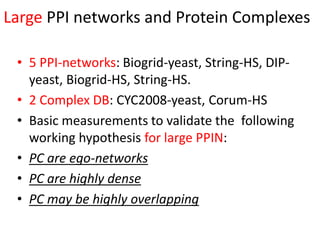
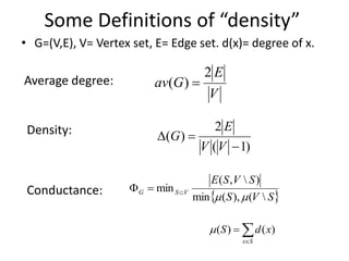
• The core decomposition CD(G) assigns to each
node in v its core number cn(v).
• cn(v)=k if v belongs to a maximal induced
subgraph of min degree k.
• cn(v) is the largest integer k you can assign to v,
so that at least k neighbors w of v in G have
cn(w)>=k.
• Observation 1: cn(v) is an upper bound to Clq(v).
• Observation 2: CD(G) can be computed in linear
time O(n+m) [Batagelj-Zaversnik, 2003].
• Thus it is a good candidate to replace the degree
as a convenient upper bound.](https://image.slidesharecdn.com/cdac2018pellegriniclusteringppinetworks-180611133039/85/CDAC-2018-Pellegrini-clustering-ppi-networks-18-320.jpg)
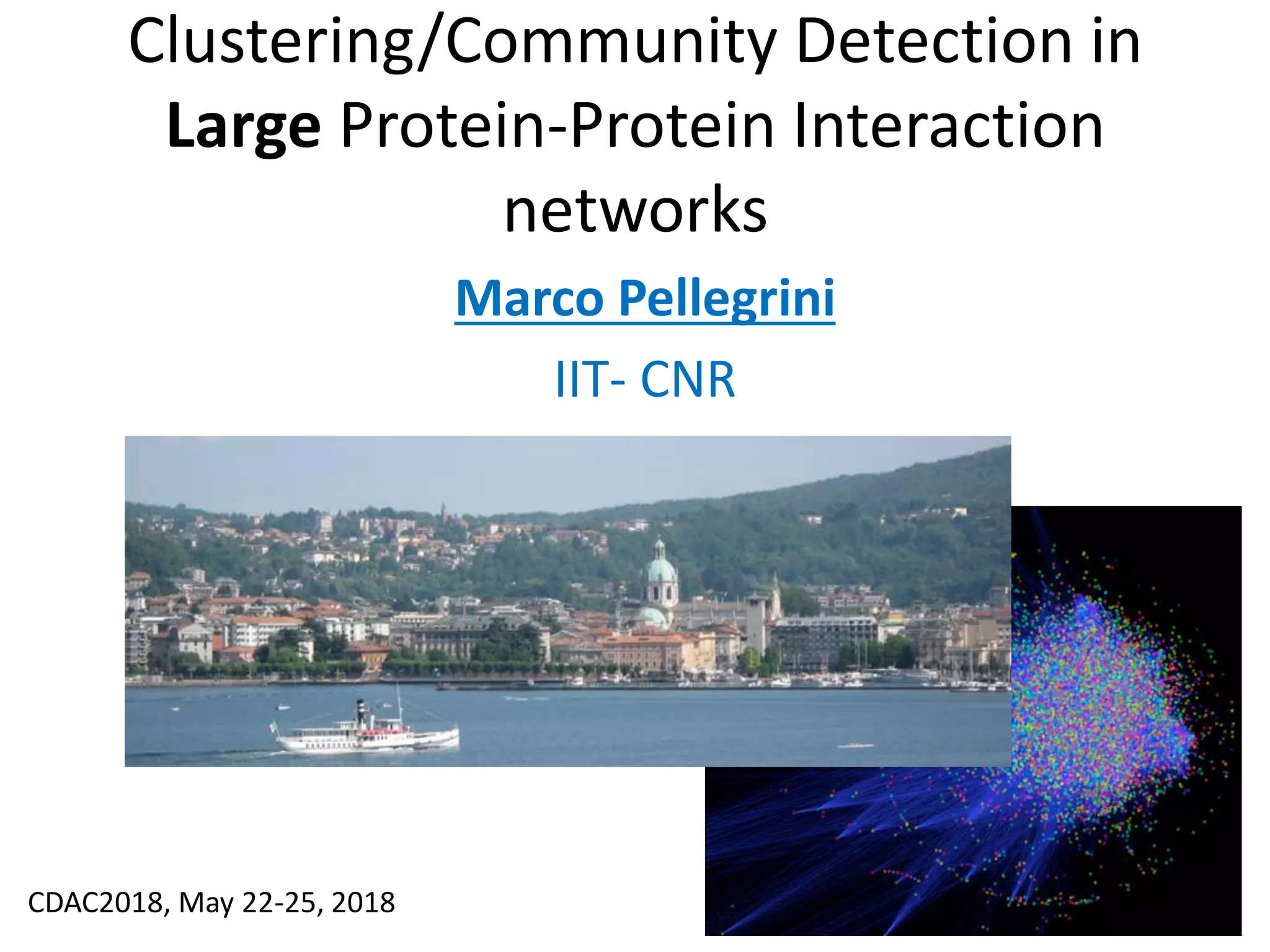
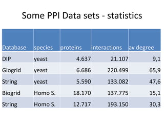
![Last phase: Charikar peeling+
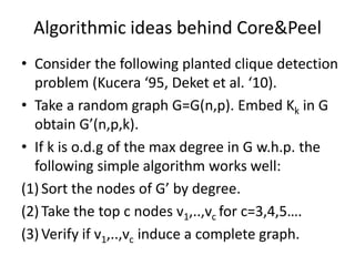
• In [Charikar 2000] it is shown that recursively
peeling the node of lowest degree in G gives a
(1/2)-approximation to the densest subgraph
(measured as average degree).
• The intuition is that if we start with a graph
that is sufficiently dense, then the optimum
densest subgraph is often the same object
with either definitions.](https://image.slidesharecdn.com/cdac2018pellegriniclusteringppinetworks-180611133039/85/CDAC-2018-Pellegrini-clustering-ppi-networks-19-320.jpg)
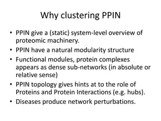
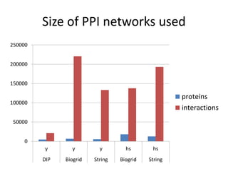
![Core&Peel in one shot
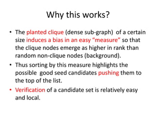
• (1) Compute the Core Decompostition of G.
• (2) Sort the vertices by decreasing core number
(solve ties by |Nr(v,c(v))|).
• (3) For each node v in turn:
• (4) Extract G[Nr(v,c(v))]
• (5) if it is above 50% density, apply Peeling+, stop
when sufficiently dense
• (6) Remove from the final output list any dense
subgraph completely included in another.
• (7) Remove from the final output almost
duplicates by Jaccard similarity above a threshold](https://image.slidesharecdn.com/cdac2018pellegriniclusteringppinetworks-180611133039/85/CDAC-2018-Pellegrini-clustering-ppi-networks-20-320.jpg)
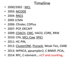
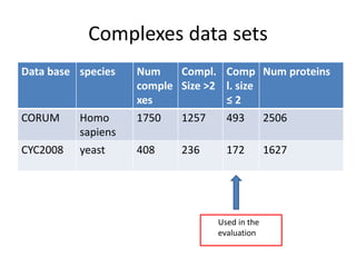
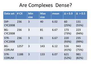
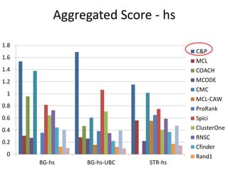
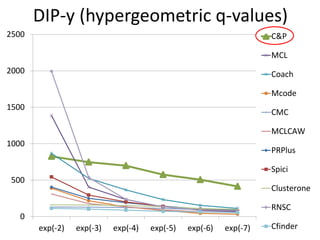
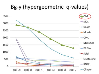
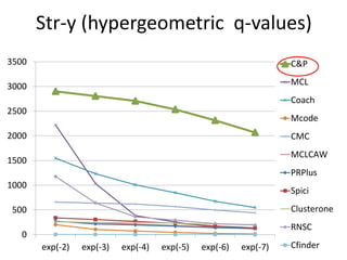
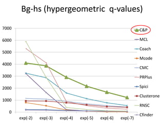
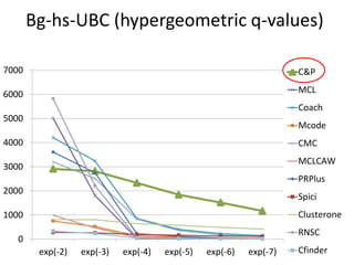
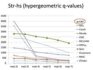
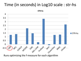
![Experiments with PPI networks
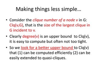
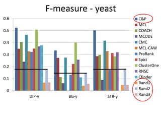
• 6 PPI-networks: Biogrid-yeast, String-HS, DIP-yeast,
Biogrid-HS, Biogrid-HS-UBC, String-HS.
• 2 Complex DB: CYC2008-yeast, Corum-HS
• 10 Competitors: MCL , COACH, MCODE, MCL-Caw,
CMC, ProRank, Spici, RNSC, ClusterOne, CFinder.
• 1 Evaluation metric : F-measure from [Li et al. BMC
genomics, 2010, 11:S3], for ω=0.2.
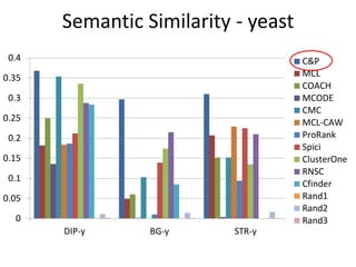
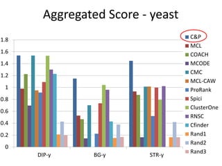
• 3 Evaluation metrics: J-measure, PR-measure, SS-
measure from [Song et al., Bioinformatics, 2009]
• Make a Aggregated Quality Index by summing them.
• Measure GO enrichment by BH-corrected p-values in
hypergoemetric tests (q-values).](https://image.slidesharecdn.com/cdac2018pellegriniclusteringppinetworks-180611133039/85/CDAC-2018-Pellegrini-clustering-ppi-networks-21-320.jpg)
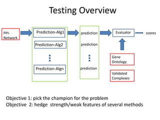


The document discusses the importance of clustering in protein-protein interaction networks (PPINs) and reviews various clustering algorithms and their evolution over time. It highlights the modular structure of PPINs, their application in understanding disease dynamics, and the use of dense sub-networks to identify functional modules. Additionally, it presents experimental results and metrics to evaluate the effectiveness of these clustering methods across multiple datasets.