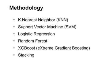
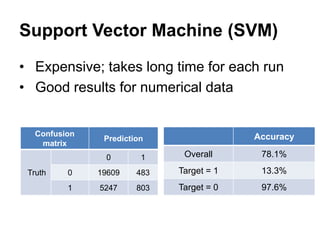
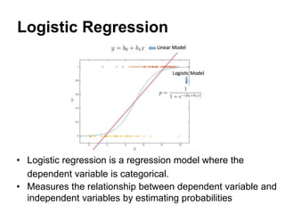
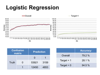
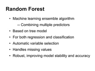
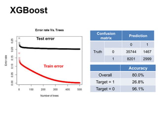
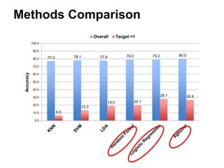
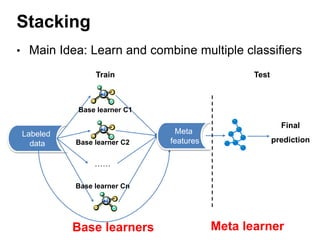
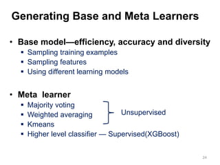
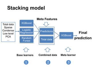
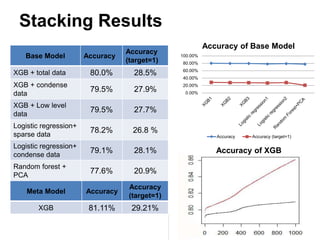
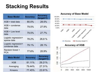
This document summarizes a team's analysis of the Springleaf lending dataset from a Kaggle competition. The team tested several classification methods including logistic regression, random forest, XGBoost, and stacking. Their best performing model was an XGBoost stacking ensemble that achieved an accuracy of 81.1% with 29.2% accuracy on the minority class. Through extensive data preprocessing and hyperparameter tuning, the team was able to improve on the winner's publicly reported accuracy of 80.4% despite their final result being 79.5%.

1. Competition II: Springleaf
Sha Li (Team leader)
Xiaoyan Chong, Minglu Ma, Yue Wang
CAMCOS Fall 2015
San Jose State University

2. Agenda
• Kaggle Competition: Springleaf dataset
introduction
• Data Preprocessing
• Classification Methodologies & Results
• Logistic Regression
• Random Forest
• XGBoost
• Stacking
• Summary & Conclusion

3. Kaggle Competition: Springleaf
Objective: Predict whether customers will
respond to a direct mail loan offer
• Customers: 145,231
• Independent variables: 1932
• “Anonymous” features
• Dependent variable:
– target = 0: DID NOT RESPOND
– target = 1: RESPONDED
• Training sets: 96,820 obs.
• Testing sets: 48,411 obs.

4. Dataset facts
• R package used to read file:
data.table::fread
• Target=0 obs.: 111,458
• Target=1 obs.: 33,773
• Numerical variables: 1,876
• Character variables: 51
• Constant variables: 5
• Variable level counts:
– 67.0% columns have
levels <= 100
Count of levels for each column
76.7%
23.3%
Class 0 and 1 count
Variables count

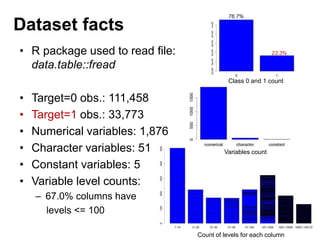
5. Missing values
• “”, “NA”: 0.6%
• “[]”, -1: 2.0%
• -99999, 96, …, 999, …,
99999999: 24.9%
• 25.3% columns have
missing values 61.7%
Count of NAs in each column Count of NAs in each row

6. Challenges for classification
• Huge Dataset (145,231 X 1932)
• “Anonymous” features
• Uneven distribution of response variable
• 27.6% of missing values
• Deal with both numerical and categorical
variables
• Undetermined portion of Categorical
variables
• Data pre-processing complexity

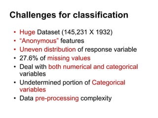
7. Data preprocessing
Remove ID and target
Replace NA by median Replace NA randomly
Replace [] and -1 as NA
Remove duplicate cols
Replace character cols
Remove low variance cols
Regard NA as a new group
Normalize Log(1+|x|)

8. Principal Component Analysis
When PC is close to 400,
it can explain 90% variance.
pc1

9. LDA: Linear discriminant analysis
• We are interested in the most discriminatory direction,
not the maximum variance.
• Find the direction that best separates the two classes.
Var1 and Var2 are large
Significant overlap
µ1 µ2
µ1 and µ2 are close

10. Methodology
• K Nearest Neighbor (KNN)
• Support Vector Machine (SVM)
• Logistic Regression
• Random Forest
• XGBoost (eXtreme Gradient Boosting)
• Stacking

11. K Nearest Neighbor (KNN)
• Target =0
• Target =1
 Overall
Accuracy
 Target = 1
Accuracy
Accuracy
72.1 73.9 75.0 76.1 76.5 76.8 77.0
22.8
18.3 15.3
12.1 10.5 9.4 7.5
0.0
10.0
20.0
30.0
40.0
50.0
60.0
70.0
80.0
90.0
100.0
3 5 7 11 15 21 39
Accuracy
K
KNN
Overall Target=1

12. Support Vector Machine (SVM)
• Expensive; takes long time for each run
• Good results for numerical data
Accuracy
Overall 78.1%
Target = 1 13.3%
Target = 0 97.6%
Confusion
matrix
Prediction
Truth
0 1
0 19609 483
1 5247 803

13. Logistic Regression
• Logistic regression is a regression model where the
dependent variable is categorical.
• Measures the relationship between dependent variable and
independent variables by estimating probabilities

14. Logistic Regression
Accuracy
Overall 79.2 %
Target = 1 28.1 %
Target = 0 94.5 %
Confusion
matrix
Prediction
Truth
0 1
0 53921 3159
1 12450 4853
75.00
75.50
76.00
76.50
77.00
77.50
78.00
78.50
79.00
79.50
80.00
2
5
15
25
35
45
55
65
75
85
95
105
115
125
135
145
155
165
175
185
195
210
240
280
320
Accuracy
PC
Overall
0.00
10.00
20.00
30.00
40.00
50.00
60.00
70.00
80.00
90.00
100.00
2
5
15
25
35
45
55
65
75
85
95
105
115
125
135
145
155
165
175
185
195
210
240
280
320
Accuracy
PC
Target=1

15. Random Forest
• Machine learning ensemble algorithm
-- Combining multiple predictors
• Based on tree model
• For both regression and classification
• Automatic variable selection
• Handles missing values
• Robust, improving model stability and accuracy

16. Random Forest
Train dataset
Draw Bootstrap
Samples
Build random
tree
Predict based
on each tree
Majority vote
A Random Tree

17. Random Forest
Accuracy
Overall 79.3%
Target = 1 20.1%
Target = 0 96.8%
Confusion
matrix
Prediction
Truth
0 1
0 36157 1181
1 8850 2223
• Target =1
• Overall
• Target =0
Tree number(500) vs Misclassification Error

18. XGBoost
• Additive tree model: add new trees that complement the already-built
ones
• Response is the optimal linear combination of all decision trees
• Popular in Kaggle competitions for efficiency and accuracy
……..
Greedy Algorithm
Number of Tree
Error
Additive tree model

19. XGBoost
• Additive tree model: add new trees that complement the already-built
ones
• Response is the optimal linear combination of all decision trees
• Popular in Kaggle competitions for efficiency and accuracy

20. XGBoost
Accuracy
Overall 80.0%
Target = 1 26.8%
Target = 0 96.1%
Train error
Test error
Confusion
matrix
Prediction
Truth
0 1
0 35744 1467
1 8201 2999

21. Methods Comparison
77.0 78.1 77.8 79.0 79.2 80.0
6.6
13.3
19.0 20.1
28.1 26.8
0.0
10.0
20.0
30.0
40.0
50.0
60.0
70.0
80.0
90.0
100.0
Accuracy
Overall Target =1

22. Winner or Combination ?

23. Stacking
Base learners Meta learner
Labeled
data
……
Final
prediction
Test
Base learner C1
Base learner C2
Base learner Cn
• Main Idea: Learn and combine multiple classifiers
Meta
features
Train

24. Generating Base and Meta Learners
• Base model—efficiency, accuracy and diversity
 Sampling training examples
 Sampling features
 Using different learning models
• Meta learner
 Majority voting
 Weighted averaging
 Kmeans
 Higher level classifier — Supervised(XGBoost)
24
Unsupervised

25. Stacking model
XGBoost
Predictions
XGBoost
Logistic
Regression
Random
Forest
Total data
Base learners Meta learner
Final
prediction
Meta Features
❶ ❸
❷
Combined data
Total data
Sparse
Condense
Low level
PCA
…

26. Stacking Results
Base Model Accuracy
Accuracy
(target=1)
XGB + total data 80.0% 28.5%
XGB + condense
data
79.5% 27.9%
XGB + Low level
data
79.5% 27.7%
Logistic regression+
sparse data
78.2% 26.8 %
Logistic regression+
condense data
79.1% 28.1%
Random forest +
PCA
77.6% 20.9%
Meta Model Accuracy
Accuracy
(target=1)
XGB 81.11% 29.21%
Averaging 79.44% 27.31%
Kmeans 77.45% 23.91%
Accuracy of XGB
0.00%
20.00%
40.00%
60.00%
80.00%
100.00%
Accuracy of Base Model
Accuracy Accuracy (target=1)

27. Stacking Results
Base Model Accuracy
Accuracy
(target=1)
XGB + total data 80.0% 28.5%
XGB + condense
data
79.5% 27.9%
XGB + Low level
data
79.5% 27.7%
Logistic regression+
sparse data
78.2% 26.8 %
Logistic regression+
condense data
79.1% 28.1%
Random forest +
PCA
77.6% 20.9%
Meta Model Accuracy
Accuracy
(target=1)
XGB 81.11% 29.21%
Averaging 79.44% 27.31%
Kmeans 77.45% 23.91%
Accuracy of XGB
0.00%
20.00%
40.00%
60.00%
80.00%
100.00%
Accuracy of Base Model
Accuracy Accuracy (target=1)

28. Summary and Conclusion
• Data mining project in the real world
 Huge and noisy data
• Data preprocessing
 Feature encoding
 Different missing value process:
New level, Median / Mean, or Random assignment
• Classification techniques
 Classifiers based on distance are not suitable
 Classifiers handling mixed type of variables are preferred
 Categorical variables are dominant
 Stacking makes further promotion
• Biggest improvement came from model selection, parameter tuning,
stacking
• Result comparison： Winner result: 80.4%
Our result: 79.5%

29. Acknowledgements
We would like to express our deep gratitude to
the following people / organization:
• Profs. Bremer and Simic for their proposal that
made this project possible
• Woodward Foundation for funding
• Profs. Simic and CAMCOS for all the support
• Prof. Chen for his guidance, valuable
comments and suggestions

30. QUESTIONS
?