Download to read offline
![Our data
caseid - pupils in school - Level 1
schoolid - schools where pupils belong - Level 2
setwd("/Volumes/DATA/RandSpatialAndArcGISNotes/MixedModels")
mydata <- read.table("5.1.txt", sep = ",", header = TRUE)
summary(mydata)[, c(1, 2)]
## caseid schoolid
## "Min. : 1 " "Min. : 1.0 "
## "1st Qu.: 8532 " "1st Qu.:123.0 "
## "Median :17318 " "Median :256.0 "
## "Mean :18466 " "Mean :254.4 "
## "3rd Qu.:29428 " "3rd Qu.:386.0 "
## "Max. :38192 " "Max. :511.0 "
Kamarul Imran M Multilevel Model - A very brief tutorial 8 December 2015 3 / 12](https://image.slidesharecdn.com/journalclubmultilevel-151212160255/75/Brief-Tutorial-on-Multilevel-Model-3-2048.jpg)
![Variables
Dependent variable is score
Covariate is cohort90 (different cohorts of pupils in schools)
summary(mydata)[,c(3,4)]
## score cohort90
## "Min. : 0.00 " "Min. :-6.0000 "
## "1st Qu.:19.00 " "1st Qu.:-4.0000 "
## "Median :33.00 " "Median :-2.0000 "
## "Mean :31.09 " "Mean : 0.2767 "
## "3rd Qu.:45.00 " "3rd Qu.: 6.0000 "
## "Max. :75.00 " "Max. : 8.0000 "
Kamarul Imran M Multilevel Model - A very brief tutorial 8 December 2015 4 / 12](https://image.slidesharecdn.com/journalclubmultilevel-151212160255/75/Brief-Tutorial-on-Multilevel-Model-4-2048.jpg)
![Dataframe
A glimpse of our data
head(mydata,4)[,1:4]
## caseid schoolid score cohort90
## 1 18 1 0 -6
## 2 17 1 10 -6
## 3 19 1 0 -6
## 4 20 1 40 -6
tail(mydata,4)[,1:4]
## caseid schoolid score cohort90
## 33985 6493 511 20 -6
## 33986 6496 511 48 -6
## 33987 6494 511 10 -6
## 33988 6495 511 0 -6
Kamarul Imran M Multilevel Model - A very brief tutorial 8 December 2015 5 / 12](https://image.slidesharecdn.com/journalclubmultilevel-151212160255/75/Brief-Tutorial-on-Multilevel-Model-5-2048.jpg)
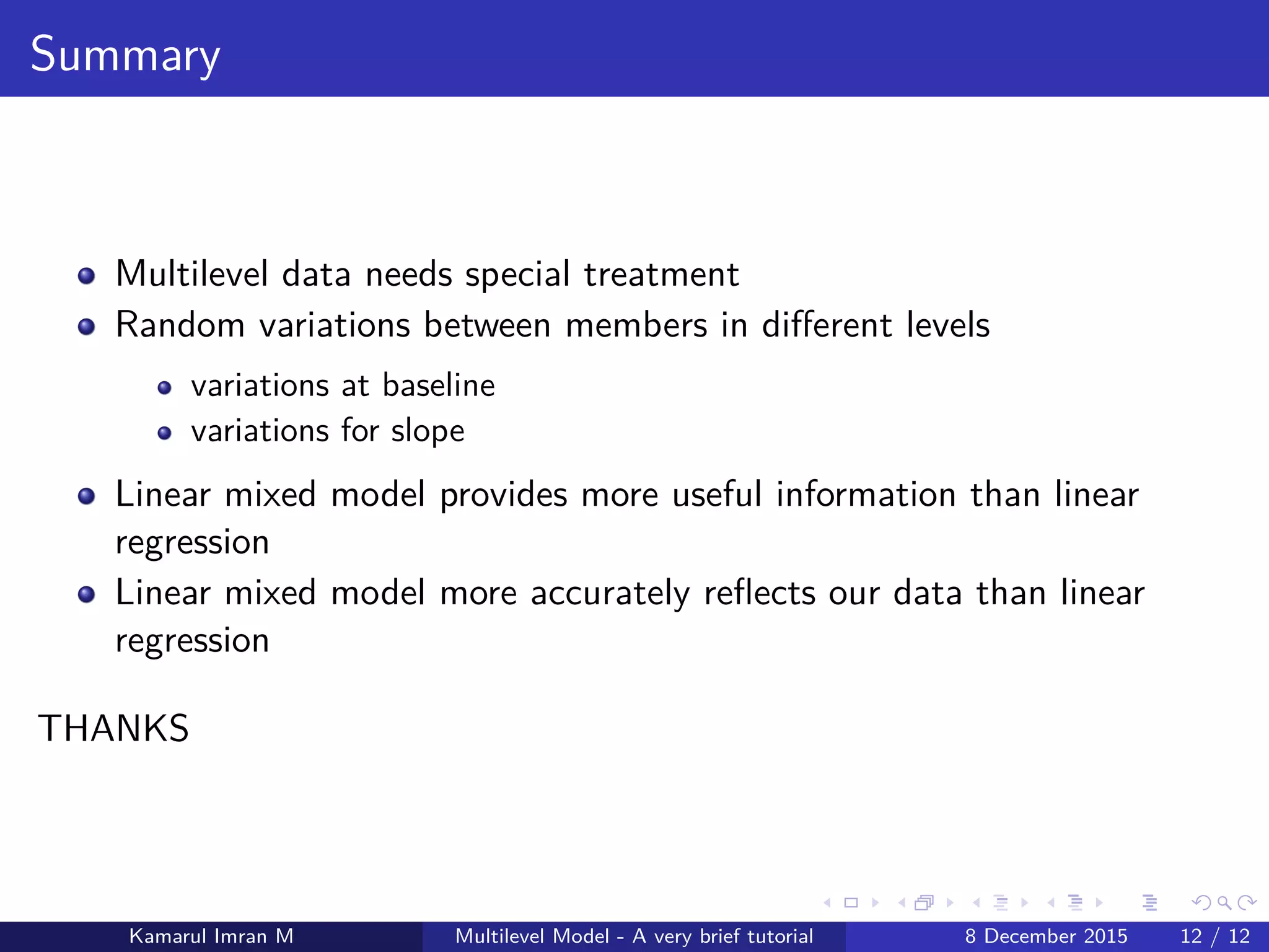

This document provides a brief tutorial on multilevel modeling, focusing on the analysis of data collected from pupils in schools across different hierarchical levels. It explains how to set up and analyze data using linear mixed models, including random intercept and random slope models, to account for variations within and between groups. The findings indicate that multilevel models offer more accurate insights compared to traditional linear regression methods.


![[DSC Europe 25] Nikolay Burlutskiy - Best Practices for Building Enterprise M...](https://cdn.slidesharecdn.com/ss_thumbnails/uirvaiuvq8y1w8hzd9tx-7-251212103249-2619edb4-thumbnail.jpg?width=640&height=640&fit=bounds)
![[DSC Europe 25] Miodrag Pesovic & Vladislav Radonjic - Federated Data Archite...](https://cdn.slidesharecdn.com/ss_thumbnails/gsbe3y5it5uhndi4e08e-1-251212103249-f1008e0c-thumbnail.jpg?width=640&height=640&fit=bounds)

![[DSC Europe 25] Dunja Adzic Jovanovic - AI and Cybersecurity: Defending Data ...](https://cdn.slidesharecdn.com/ss_thumbnails/o1zylpbhrtwnixxq2xj8-7-251211083048-185086f6-thumbnail.jpg?width=640&height=640&fit=bounds)


![[DSC Europe 25] Branko Urosevic -Rethinking Financial Talent: Integrating Cod...](https://cdn.slidesharecdn.com/ss_thumbnails/8jjrus8ttko6qj64f58f-3-251212103250-642c6374-thumbnail.jpg?width=640&height=640&fit=bounds)


![[DSC Europe 25] Marko Krstic - Understanding the AI Threat Landscape - Risks,...](https://cdn.slidesharecdn.com/ss_thumbnails/tiyim1ins5jvbrvzpzla-2-251209104645-c69d3553-thumbnail.jpg?width=640&height=640&fit=bounds)
![[DSC Europe 25] Behzad Hosseini - AI Agents in the Wild: Deploying Models tha...](https://cdn.slidesharecdn.com/ss_thumbnails/3qtejajvsjqrzwfept2c-10-251212103250-7f2b1068-thumbnail.jpg?width=640&height=640&fit=bounds)
![[DSC Europe 25] Jon Dajci - Bridging TradFi and DeFi: Building the Future of ...](https://cdn.slidesharecdn.com/ss_thumbnails/fqmhfvlbqhkihjvqvhmu-7-251211083849-6af7e325-thumbnail.jpg?width=640&height=640&fit=bounds)
![[DSC Europe 25] Hans Kleinsman - The Compliance Gearbox: How Tax Tech Mediate...](https://cdn.slidesharecdn.com/ss_thumbnails/dxdytie1toel0hr90bjs-2-251212103250-174fdbe7-thumbnail.jpg?width=640&height=640&fit=bounds)

