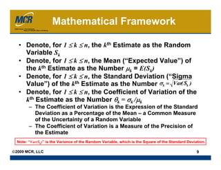
More Related Content
Similar to Book.steve (20)
Book.steve
- 1. Combining
Probabilistic Estimates
to Reduce Uncertainty
Stephen A. Book
Chief Technical Officer
MCR, LLC, 390 No. Sepulveda Blvd.
El Segundo CA 90245
(424) 218-1613
sbook@mcri.com
National Aeronautics and Space Administration
Program Management Challenge 2009
©2009 MCR, LLC Daytona Beach FL, 24-25 February 2009
- 2. Acknowledgments
The analysis presented in this document has its
origin in a question posed to the author by Mr. Claude
Freaner of the Science Directorate at NASA
Headquarters, Washington DC.
Mr. Nathan Menton of MCR conducted a
thorough quality review of the mathematics formulated
herein, leading to a significant improvement in the
specific details of the conclusions drawn.
Dr. Neal Hulkower and Mr. John Neatrour of
MCR also contributed several valuable suggestions as
part of the quality review.
©2009 MCR, LLC 2
- 3. Contents
• Objective and Assumptions
• A Basic Mathematical Fact
• The Case of Three S-Curve Estimates
• A Numerical Example
• An Excursion
• The Excursion via Weighted Averaging
• The General Case
• Summary
©2009 MCR, LLC 3
- 4. Contents
• Objective and Assumptions
• A Basic Mathematical Fact
• The Case of Three S-Curve Estimates
• A Numerical Example
• An Excursion
• The Excursion via Weighted Averaging
• The General Case
• Summary
©2009 MCR, LLC 4
- 5. What a Cost Estimate
Looks Like
Percentile Value Program Alpha
10% 516.81 10,000 Trials Cumulative Chart
1.000
20% 538.98
“S-Curve”
30% 557.85 .750
40% 575.48
.500
50% 592.72
60% 609.70 .250
70% 629.19 .000
80% 650.97 462.43 537.16 611.89
BY04$M
686.62 761.35
90% 683.01
Program Alpha
10,000 Trials Frequency Chart
Statistics Value .020
Trials 10,000 “Density Curve”
Mean 596.40 .015
Density
Median 592.72 .010
Mode ---
Standard Deviation 63.18 .005
Range Minimum 450.19
Range Maximum 796.68 .000
462.43 537.16 611.89 686.62 761.35
BY04$M
©2009 MCR, LLC 5
- 6. Objective of the Study
• We Have n Estimates, Independent of Each
Other, of the Same System or Project
• The Estimates are Expressed Statistically –
Their S-Curves, Means, and Standard
Deviations are Known
• We Want to Combine These n Estimates to
Obtain One Estimate that Contains Less
Uncertainty than Each of the n Estimates
Individually
• Question: Will the Combined Estimate Actually
be Less Uncertain than Each of the n
Independent Estimates Individually
©2009 MCR, LLC 6
- 7. Assumptions
• The n Estimates are Independent of Each Other
• We Know Each of their Means, Standard Deviations,
and therefore their Coefficients of Variation (=
Standard Deviation ÷ Mean)
• The Estimates are “Credible,” i.e. …
– They are Based on the Same Technical Description of the
Program and on Risk Assessments Validly Drawn from the
Same Risk Information Available to Each Estimating Team
– Each Estimating Team Applied Appropriate Mathematical
Techniques to Obtain the Estimate and Conduct the Cost-
Risk Analysis, Including (for example) Inter-Element
Correlations when Appropriate
– Each Estimating Team Worked from the Same Ground Rules,
but May Have Applied Different Estimating Methods and
Made Different Assumptions when Encountering the Absence
of Some Required Information
©2009 MCR, LLC 7
- 8. A Note on “Credibility”
• A Cost Estimate is “Credible” if it is Based on …
– A Valid Technical and Programmatic Description of the Item
or Program to be Costed
– Application of Valid Mathematical Techniques that Produce
Cost Estimates from Technical and Programmatic
Information
– An Assessment of Program Risks by Knowledgeable
Engineers and their Translation into Cost Impacts by
Knowledgeable Cost Analysts
– Application of Valid Statistical Methods in “Rolling Up” WBS-
Cost Probability Distributions into a Total-Cost Probability
Distribution
• Whether or Not an Estimate is Credible does not
Depend on its Accuracy or Precision
• All Estimates Remaining after the Reconciliation
Process Has Been Completed Should be Considered
Credible
©2009 MCR, LLC 8
- 9. Mathematical Framework
• Denote, for 1 ≤ k ≤ n, the kth Estimate as the Random
Variable Sk
• Denote, for 1 ≤ k ≤ n, the Mean (“Expected Value”) of
the kth Estimate as the Number μk = E(Sk)
• Denote, for 1 ≤ k ≤ n, the Standard Deviation (“Sigma
Value”) of the kth Estimate as the Number σk = Var( Sk )
• Denote, for 1 ≤ k ≤ n, the Coefficient of Variation of the
kth Estimate as the Number θk = σk /μk
– The Coefficient of Variation is the Expression of the Standard
Deviation as a Percentage of the Mean – a Common Measure
of the Uncertainty of a Random Variable
– The Coefficient of Variation is a Measure of the Precision of
the Estimate
Note: “Var(Sk)” is the Variance of the Random Variable, which is the Square of the Standard Deviation.
©2009 MCR, LLC 9
- 10. Contents
• Objective and Assumptions
• A Basic Mathematical Fact
• The Case of Three S-Curve Estimates
• A Numerical Example
• An Excursion
• The Excursion via Weighted Averaging
• The General Case
• Summary
©2009 MCR, LLC 10
- 11. A Basic Mathematical Fact
Theorem: If, for 1 ≤ k ≤ n, the numbers μk are all
positive, then
2
n
⎛ ⎞ n
∑ μ < ⎜ ∑ μk ⎟ .
2
k⎜ ⎟
Proof: k =1 ⎝ k =1 ⎠
( )
2
⎛ n ⎞2
⎜ ∑ μk ⎟ = μ + μ + μ +
⎜ ⎟ • • •
1 2 3
⎝ k =1 ⎠
= μ 12 + μ 2 + μ 3 +
2 2
• • • + 2 μ 1μ 2 + 2 μ 1μ 3 + 2 μ 2 μ 3 + • • •
n
> μ 12 + μ 2 + μ 3 +
2 2
• • • = ∑μ
k =1
2
k
QED
Recall from Algebra: (a+b)2 = a2 + b2 + 2ab.
©2009 MCR, LLC 11
- 12. Contents
• Objective and Assumptions
• A Basic Mathematical Fact
• The Case of Three S-Curve Estimates
• A Numerical Example
• An Excursion
• The Excursion via Weighted Averaging
• The General Case
• Summary
©2009 MCR, LLC 12
- 13. Example: The Case of Three
Independent Estimates
• Suppose We Have Three Independent (of each other) Probabilistic
Estimates of the Same System or Project: S1 , S2 , S3
• The Statistical Average (Mean) of the Three Estimates is
S + S2 + S3
S= 1
3
• Because the Mean of a Sum is the Sum of the Means (a statistical
theorem), We Know that the Mean of the Average Estimate is
()
μ=E S = 1
μ + μ2 + μ3
3
• Furthermore, the Variance of a Sum of Independent Random
Variables is the Sum of the Individual Variances with Any Constant
Divisor or Multiple Squared, We See that
Var (S 1 ) + Var (S 2 ) + Var (S 3 ) σ 12 + σ 2 + σ 3
()
2 2
σ = Var S =
2
=
9 9
©2009 MCR, LLC 13
- 14. The Role of the
Coefficients of Variation
• Suppose θ1 = σ1 /μ1, θ2 = σ2/μ2, and θ3 = σ3 /μ3 are the
Respective Coefficients of Variation – the Three
Standard Deviations Expressed as Percentages of
their Corresponding Means
• Then the Standard Deviation of the Average Estimate
Can be Expressed as
σ 12 + σ 22 + σ 32 1 1
σ= = σ1 +σ2 +σ3 =
2 2 2
θ 12 μ 12 + θ 22 μ 2 + θ 32 μ 32
2
9 3 3
• Now Suppose We Denote by θ the Coefficient of
Variation of the Average of the Three Estimates –
Then 1
θ 2μ 2 + θ 2μ 2 + θ 2μ 2
σ 1 1 2 222 232 232
θ1 μ1 + θ2 μ2 + θ3 μ3
θ = = 3 =
μ 1
(μ 1 + μ 2 + μ 3 ) (μ 1 + μ 2 + μ 3 )
3
©2009 MCR, LLC 14
- 15. The Relative Uncertainty of
the Average Estimate
• Use the Symbol λ to Denote the Ratio of the
Uncertainty (as expressed by the coefficient of
variation) of the Average Estimate to the
Uncertainty of the “Best” (smallest uncertainty)
Original Estimate
• Algebraically, this Means that
θ θ 12 μ12 + θ 22 μ 2 + θ 32 μ 3
2 2
λ= =
min( θ 1 ,θ 2 ,θ 3 ) (μ1 + μ 2 + μ 3 ) × min( θ 1 ,θ 2 ,θ 3 )
• Therefore the Uncertainty of the Average Estimate
is λ × min(θ1, θ2,θ3)
©2009 MCR, LLC 15
- 16. Contents
• Objective and Assumptions
• A Basic Mathematical Fact
• The Case of Three S-Curve Estimates
• A Numerical Example
• An Excursion
• The Excursion via Weighted Averaging
• The General Case
• Summary
©2009 MCR, LLC 16
- 17. A Numerical Example with
Equal Coefficients of Variation
• Suppose We Have Three Independent Probabilistic
Estimates of a System or Project
• Suppose the Three Means are μ1 = 400, μ2 = 500, and μ3 =
600 Million Dollars, Respectively
• Suppose the Three Coefficients of Variation are All 20%,
i.e., θ1 = 0.20, θ2 = 0.20, and θ3 = 0.20, Respectively
• This Implies that the Three Standard Deviations are,
Respectively, σ1 = 80, σ2 = 100, and σ3 = 120
• Then the Average Estimate is μ = (400+500+600)/3 = 500,
and its Standard Deviation is
1 1 1
σ= σ 12 + σ 2 + σ 3 =
2 2
6400 + 10000 + 14400 = 30800 = 58.5
3 3 3
• This Implies that the Coefficient of Variation of the Average
Estimate is θ = σ/μ = 58.5/500 = 0.117 = 11.7%, so that the
Average Estimate Has Less Uncertainty than Each of the
Three Original Estimates
©2009 MCR, LLC 17
- 18. An Alternative Calculation
• We Can Make the Same Calculation by Going Directly to the
Expression for λ
• The Ratio of the Uncertainty (as expressed by the coefficient
of variation) of the Average Estimate to the Uncertainty of the
“Best” (smallest uncertainty) Original Estimate is
θ θ 12 μ 12 + θ 22 μ 22 + θ 32 μ 32
λ = =
min( θ 1 , θ 2 , θ 3 ) (μ 1 + μ 2 + μ 3 ) × min( θ 1 , θ 2 , θ 3 )
( 0 .20 2 )( 400 2 ) + ( 0 . 20 2 )( 500 2 ) + ( 0 .20 2 )( 500 2 )
=
(400 + 500 + 600 ) × min( 0 .20 ,0 .20 ,0 .20 )
( 0 .04 )( 160000 ) + ( 0 .04 )( 250000 ) + ( 0 .04 )( 360000 )
=
(1500 ) × 0 .20
6400 + 10000 + 14400 30800
= = = 0 . 585
300 300
• Therefore the Resulting Uncertainty of the Average Estimate
is λ×min(θ1,θ2,θ3) = 0.585×0.20 = 0.117 = 11.7%
©2009 MCR, LLC 18
- 19. What Do We Conclude About
Our Numerical Example?
• We Began with Three Independent (from each
other) Probabilistic Estimates, the Standard
Deviation of Each of which was 20% of its
Respective Mean
• Upon Averaging the Means of Each of the Three
Estimates, We Obtained an Estimate whose
Standard Deviation was Only 11.7% of the Mean
• In this Case, therefore, We Were Able to Use the
Three Estimates to Derive One Estimate that Has
Less Uncertainty than Each of the Three Original
Estimates
©2009 MCR, LLC 19
- 20. Contents
• Objective and Assumptions
• A Basic Mathematical Fact
• The Case of Three S-Curve Estimates
• A Numerical Example
• An Excursion
• The Excursion via Weighted Averaging
• The General Case
• Summary
©2009 MCR, LLC 20
- 21. An Excursion
• Suppose We Have Three Probabilistic Estimates of a
System or Project as Before, whose Three Means are
μ1 = 400, μ2 = 500, and μ3 = 600 Million Dollars,
Respectively, as Before
• However, Suppose the Three Coefficients of Variation
are Now, Respectively, θ1 = 10%, θ2 = 30%, and θ3 =
50%
• This Implies that the Three Standard Deviations are,
Respectively, σ1 = 40, σ2 = 150, and σ3 = 300
• The Average Estimate is Again μ = (400+500+600)/3 =
500, but its Standard Deviation is Now
1 1 1
σ= σ1 +σ2 +σ3 =
2 2 2
1600 + 22500 + 90000 = 114100 = 112 .6
3 3 3
©2009 MCR, LLC 21
- 22. Naïve Analysis of the Excursion
• All This Implies that the Coefficient of Variation
of the Average Estimate is θ = σ/μ = 112.6/500
= 0.225 = 22.5%, so that the Average Estimate
Has Less Uncertainty than Two of the Three
Original Estimates, but not the Third
• In this Case, It Appears we would be Better Off
(at least with respect to uncertainty) by Using
the First Estimate (which has a 10% coefficient
of variation) than to Average the Three
Estimates
©2009 MCR, LLC 22
- 23. Contents
• Objective and Assumptions
• A Basic Mathematical Fact
• The Case of Three S-Curve Estimates
• A Numerical Example
• An Excursion
• The Excursion via Weighted Averaging
• The General Case
• Summary
©2009 MCR, LLC 23
- 24. Fixing the Excursion by
Weighting the Estimates
• Because the Three Estimates in the Excursion are of Different
Levels of Precision, to Combine Them We Should Really be
Calculating their “Weighted Average” (weighted by precision),
rather than their Straight Average
• Again, Suppose the Three Means are μ1 = 400, μ2 = 500, and μ3 =
600 Million Dollars, Respectively, as Before, and the Three
Coefficients of Variation are, Respectively, θ1 = 10%, θ2 = 30%, and
θ3 = 50%, again as Before
• This again Implies that the Three Standard Deviations are,
Respectively, σ1 = 40, σ2 = 150, and σ3 = 300
• Suppose Now We Calculate the Weighted Average Estimate
(denoted by W ), Using the Coefficients of Variation as the
Respective Weights – in Particular,
μ1 μ 2 μ 3
+ +
θ1 θ2 θ3
W=
1 1 1
+ +
©2009 MCR, LLC
θ1 θ2 θ3 24
- 25. Calculating the
Weighted Average
• The Formula for the Weighted Average Counts Less
Uncertain Estimates, i.e. those Having a Smaller
Coefficient of Variation, More Heavily in the Average
• Let’s Now Calculate the Weighted Average Estimate:
μ1 μ 2 μ 3
400 500 600
+ + + +
θ1 θ 2 θ 3
0.10 0.30 0.50 = 4000 + 1666.66667 + 1200
W= =
1 1 1
+ +
1
+
1
+
1 10 + 3.33333 + 2
θ1 θ 2 θ 3 0.10 0.30 0.50
6866.66667
= = 447.82618
15.33333
• Note that the Weighted Average is Closer to 400 than is
the “Unweighted” Average, because the 400 is
Weighted More Heavily than Either the 500 or 600
©2009 MCR, LLC 25
- 26. Variance of the
Weighted Average
• The Weighted Average is Really the Expected
Value of the Weighted Probabilistic Estimate,
which is S1 S 2 S 3
+ +
θ1 θ2 θ3
W =
1 1 1
+ +
θ1 θ2 θ3
• The Variance of the Weighted Estimate then
has the formula
⎛S S S ⎞ 1
Var(S1 ) + 2 Var(S2 ) + 2 Var(S3 )
1 1
Var⎜ 1 + 2 + 3 ⎟
⎜
⎝ θ1 θ2 θ3 ⎟ θ12
⎠= θ2 θ3
Var( W ) = 2 2
⎛1 1 1⎞ ⎛1 1 1⎞
⎜ + + ⎟
⎜θ θ θ ⎟ ⎜ + + ⎟
⎜θ θ θ ⎟
⎝ 1 2 3⎠ ⎝ 1 2 3⎠
©2009 MCR, LLC 26
- 27. Standard Deviation of the
Weighted Average
• Because the Three Means are μ1 = 400, μ2 = 500, and μ3 = 600
Million Dollars, Respectively, and the Three Coefficients of
Variation are θ1 = 10%, θ2 = 30%, and θ3 = 50%, Respectively, We
See that the Three Standard Deviations are σ1 = 40, σ2 = 150, and
σ3 = 300, Respectively
• Therefore the Variance of the Weighted Average is
40 2 150 2 300 2
Var (S1 ) + Var (S2 ) + Var (S3 )
1 1 1
+ +
θ 12 θ 22 θ 32 ( 0.10 )2 ( 0.30 )2 ( 0.50 )2
Var( W ) = 2 = 2
⎛1 1 1⎞ ⎛ 1 1 1 ⎞
⎜θ + θ + θ ⎟
⎜ ⎟ ⎜ + + ⎟
⎝ 1 2 3 ⎠ ⎝ 0.10 0.30 0.50 ⎠
160 ,000 + 250 ,000 + 360 ,000 770 ,000
= = = 3 ,275.04868
(10 + 3.33333 + 2 )2 ( 15.33333 )2
• It Follows that the Standard Deviation of the Weighted Average of
the Three Estimates is the Square Root of 3,275.05, namely 57.23
©2009 MCR, LLC 27
- 28. Coefficient of Variation
of the Weighted Average
• On Previous Slides, We Found that W = 447.83 and σ(W)
= 57.23
• It therefore Follows that the Coefficient of Variation of
the Weighted Average is
σ ( W ) 57.22804
θW = = = 0.12779 = 12.78%
W 447.82618
• The Lesson Here Seems to be that, if We Use
Coefficients of Variation to Weight these Particular
Statistically Independent Probabilistic Estimates
– … the Weighted Estimate has Significantly Less Uncertainty
than the Unweighted “Average” Estimate (whose coefficient of
variation was 22.5%)
– … and Less Uncertainty than Two of the Three Original
Estimates
– … but Still not Less Uncertainty than the Least Uncertain of the
Three Original Estimates
©2009 MCR, LLC 28
- 29. Contents
• Objective and Assumptions
• A Basic Mathematical Fact
• The Case of Three S-Curve Estimates
• A Numerical Example
• An Excursion
• The Excursion via Weighted Averaging
• The General Case
• Summary
©2009 MCR, LLC 29
- 30. The General Case
• Suppose We Have Three Independent
Probabilistic Estimates of a System or Project
– Suppose the Three Means are μ1, μ2, and μ3
– Suppose the Three Coefficients of Variation are, Respectively,
θ1, θ2, and θ3
– This Implies that the Three Standard Deviations are,
Respectively, σ1 = θ1μ1, σ2 = θ2μ2, and σ3 = θ3μ3
• We Can Assume, without Loss of Generality,
that θ1 ≤ θ2 ≤ θ3
– Furthermore, We Can Set θ2 = αθ1 and θ3 = βθ1
– It Therefore Follows that 1 ≤ α ≤ β
• This Leads to σ1 = θ1μ1, σ2 = αθ1μ2, and σ3 =
βθ1μ3
©2009 MCR, LLC 30
- 31. Weighting the Estimates
in the General Case
• Suppose Now We Calculate the Weighted Average
Estimate (denoted by W), Using the Coefficients of
Variation as the Respective Weights – in Particular,
μ1 μ2 μ3 μ1 μ2 μ3
+ + + +
θ1 θ2 θ3 θ 1 αθ 1 βθ 1
W = =
1 1 1 1 1 1
+ + + +
θ1 θ2 θ3 θ1 αθ 1 βθ 1
1 ⎛ μ2 μ3 ⎞ μ2 μ3
⎜ μ1 + + ⎟ μ1 + +
θ1 ⎝ α β ⎠ α β
= =
1 ⎛ 1 1 ⎞ 1+
1
+
1
⎜1+ + ⎟
θ1 ⎝ α β ⎠ α β
©2009 MCR, LLC 31
- 32. Calculating the Variance of
the Weighted Average Estimate
• As Before, the Weighted Average Estimate is Really
the Expected Value of the Weighted Probabilistic
Estimate, which is
S1 S2 S3 S1 S2 S3 S2 S3
+ + + + S1 + +
θ1 θ2 θ3 θ1 αθ βθ α β
W = = 1 1
=
1 1 1 1 1 1 1 1
+ + + + 1+ +
θ1 θ2 θ3 θ1 αθ 1 βθ 1 α β
• In the Current Situation, the Variance of the Weighted
Average Estimate is then (since the estimates are
assumed to be independent)
⎛ S S ⎞
Var⎜ S1 + 2 + 3 ⎟ Var (S1 ) + 2 Var (S2 ) + 2 Var (S3 )
1 1
⎝ α β ⎠ α β
Var( W ) = 2
= 2
⎛ 1 1⎞ ⎛ 1 1⎞
⎜1+ + ⎟ ⎜1+ + ⎟
⎝ α β⎠ ⎝ α β⎠
©2009 MCR, LLC 32
- 33. The Variance of the
Weighted Average Estimate
• Continuing the Calculation on the Previous Chart and
Recalling that σ1 = θ1μ1, σ2 = αθ1μ2, and σ3 = βθ1μ3,
We See that
Var (S1 ) + Var (S2 ) + Var (S3 )
1 1
α 2
β 2
Var ( W ) = 2
⎛ 1 1⎞
⎜1+ + ⎟
⎝ α β⎠
(θ 1μ 1 ) + 2 (αθ 1μ 2 ) + 2 (βθ 1μ 3 )2
2 1 2 1
α β θ 12 (μ 12 + μ 22 + μ 32 )
= 2 = 2
⎛ 1 1⎞ ⎛ 1 1⎞
⎜1+ + ⎟ ⎜1+ + ⎟
⎝ α β⎠ ⎝ α β⎠
©2009 MCR, LLC 33
- 34. Coefficient of Variation of the
Weighted Average Estimate
σW Var
• It Follows from the Aforementioned
( ) (W
)
θ= =
Calculations that the Coefficient of Variation
of the Weighted Average Estimate is
W =
θ 12 (μ 12 + μ 22 + μ 3 )
W W
2
2
⎛ 1 1⎞
⎜1+ + ⎟
σ (W ) Var ( W ) ⎝ α β⎠ θ 1 μ 12 + μ 2 + μ 32
2
θW = = = =
W W μ2 μ3 μ μ
μ1 + + μ1 + 2 + 3
α β α β
1 1
1+ +
α β
©2009 MCR, LLC 34
- 35. When is the Weighted Average
Estimate a “Better” Estimate?
• According to Our Criterion, We Will Consider the
Weighted Average Estimate to be a “Better”
σW Var
( ) (W
)
θ= = =
Estimate than the Best of the Three Original
Estimates if it is Less Uncertain
• This Will Happen if θW < θ1, namely if
W
θ 1 μ 12 + μ 22 + μ 3
2 W W
< θ1
μ2 μ3
μ1 + +
α β
According to the Calculation on the Previous Chart
μ2 μ3
• And so, if μ + μ + μ < μ1 +
2 2 2
+
1 2 3
α β
μ2 μ3
• … or if, Equivalently, μ 1 + μ 2 + μ 3 − μ 1 − − <0
2 2 2
α β
©2009 MCR, LLC 35
- 36. Applying the General-Case Test
to the First Numerical Example
• Our Test Will Assert that the Weighted Average
Estimate is a “Better” Estimate than the Best of the
σW Var
( ) (W
)
θ= = =
Three Original Estimates if
μ2 μ3
μ12 + μ2 + μ3 − μ1 −
2 2
− <0
α β W
• In Our First Numerical Example, μ1 = 400, μ2 = 500, and
μ3 = 600 and θ1 = 20%, θ2 = 20%, and θ3 = 20% W W
• It Follows that α = 1 and β = 1, so that
μ2 μ3 500 600
μ 12 + μ 22 + μ 32 − μ 1 − − = 400 2
+ 500 2
+ 600 2
− 400 − −
α β 1 1
= 770 ,000 − 400 − 500 − 600
= 877 . 49644 − 1 ,500 = − 622 . 50536
• Since the Answer is a Negative Number, the Test’s
Advice is to Use the Weighted Average Estimate as
the Cost Estimate
©2009 MCR, LLC 36
- 37. Applying the General-Case Test
to the Excursion Example
• Our Test Will Assert that the Weighted Average
Estimate is a “Better” Estimate than the Best of the
σW Var
( ) (W
)
θ= = =
Three Original Estimates if
μ2 μ3
μ12 + μ2 + μ3 − μ1 −
2 2
− <0
α β
W
• In Our Excursion Example, μ1 = 400, μ2 = 500, and μ3 =
600 and θ1 = 10%, θ2 = 30%, and θ3 = 50%
W W
• It Follows that α = 3 and β = 5, so that
μ2 μ3 500 600
μ 12 + μ 22 + μ 32 − μ 1 − − = 400 2 + 500 2 + 600 2 − 400 − −
α β 3 5
= 770 ,000 − 400 − 166 .66667 − 120
= 877 .49644 − 686 .66667 = 190 .82977
• Since the Answer is a Positive Number, the Test’s
Advice is to Stick with the Best of the Three Original
Estimates
©2009 MCR, LLC 37
- 38. Contents
• Objective and Assumptions
• A Basic Mathematical Fact
• The Case of Three S-Curve Estimates
• A Numerical Example
• An Excursion
• The Excursion via Weighted Averaging
• The General Case
• Summary
©2009 MCR, LLC 38
- 39. Summary
• Suppose We Have Three Independent Probabilistic
Estimates of a System or Project
– Suppose the Three Means are μ1, μ2, and μ3
– Suppose the Three Coefficients of Variation are,
Respectively, θ1, θ2, and θ3, where θ1 ≤ θ2 ≤ θ3 ,
– … so that the Three Standard Deviations are, Respectively,
σ1 = θ1μ1, θ2 = αθ1μ2, and σ3 = βθ1μ3, where 1 ≤ α ≤ β
• Our Test Recommends that the Weighted Average
Estimate be Used if
μ2 μ3
μ + μ + μ − μ1 −
2 2 2
− <0
1 2 3
α β
and the Best of the Three Original Estimates be Used
Otherwise
• The Formulas Easily Generalize to Cover the Case of
More (or Fewer) than Three Independent Estimates
©2009 MCR, LLC 39
- 40. Conclusion
• If Reducing Uncertainty in Your Estimate is
Your Goal, and You Have Several Valid
Independent Estimates to Choose from,
– Is it Better to Average Multiple Estimates or
– Is it Better Simply to Use the “Best” of Them?
• If the Several Estimates Vary in Uncertainty,
We Have Established a Numerical Test to
Determine Whether the Weighted (by their
respective coefficients of variation) Average
Estimate Has Less Uncertainty than the Least
Uncertain of the Original Estimates
©2009 MCR, LLC 40