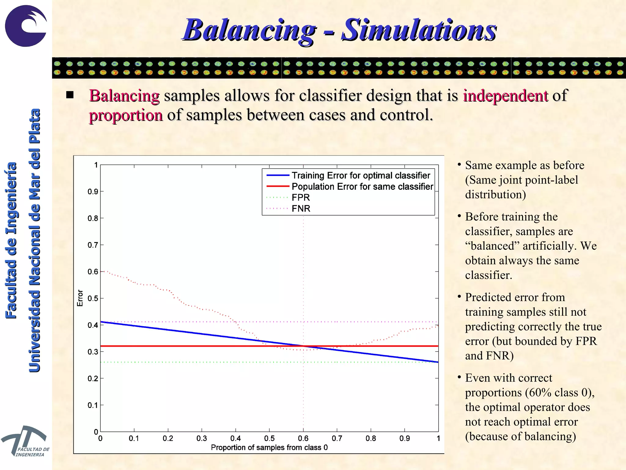
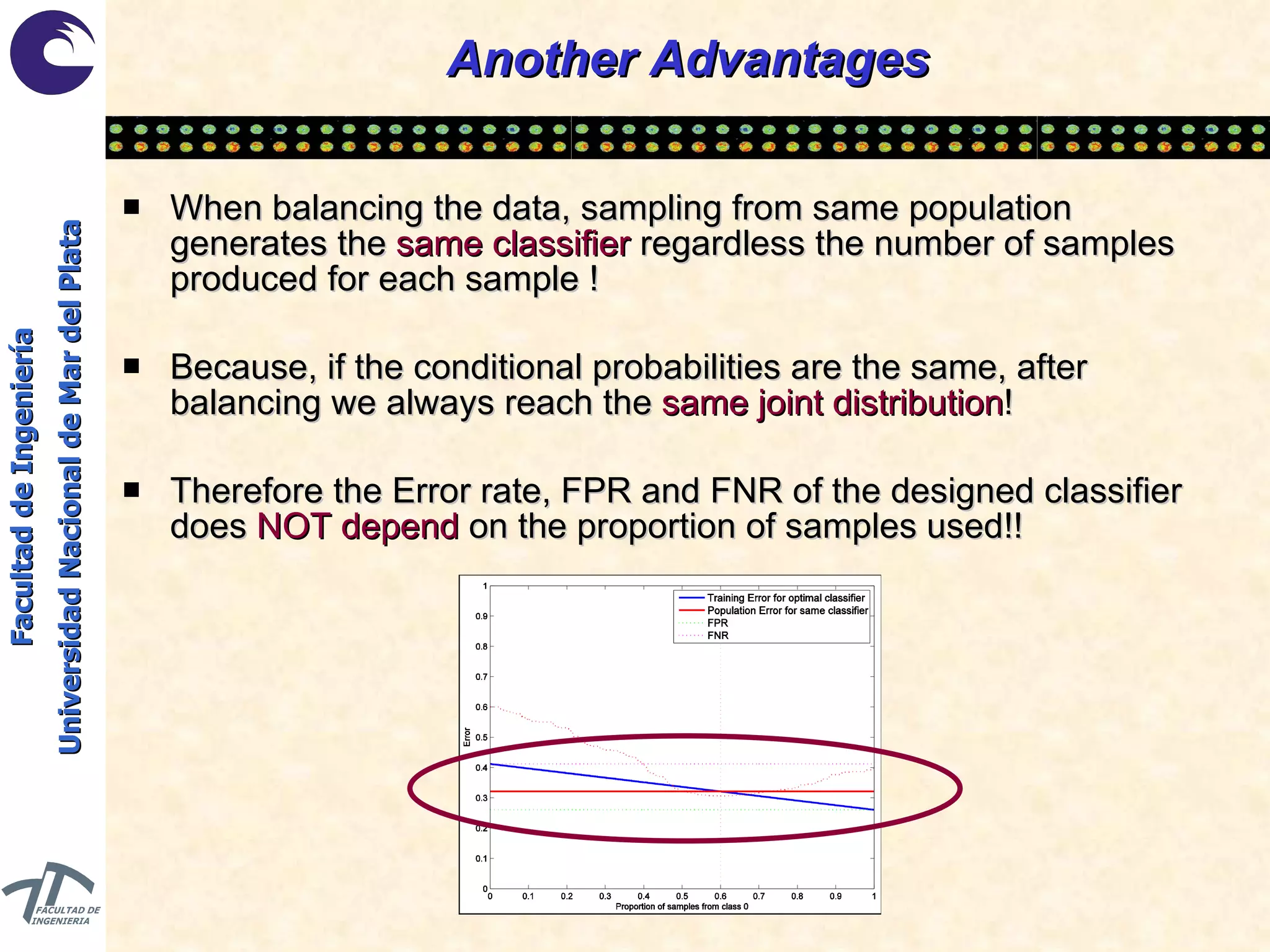
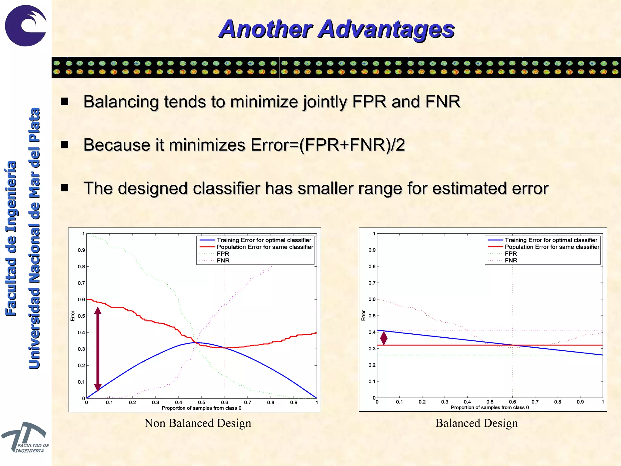
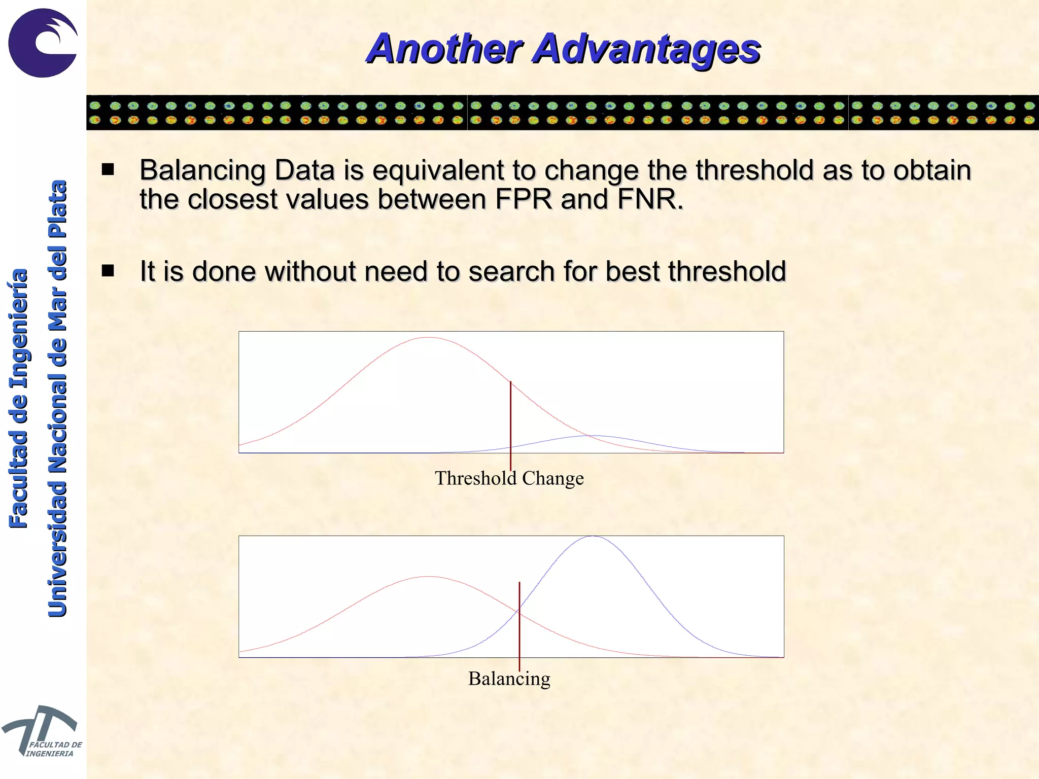
Download to read offline
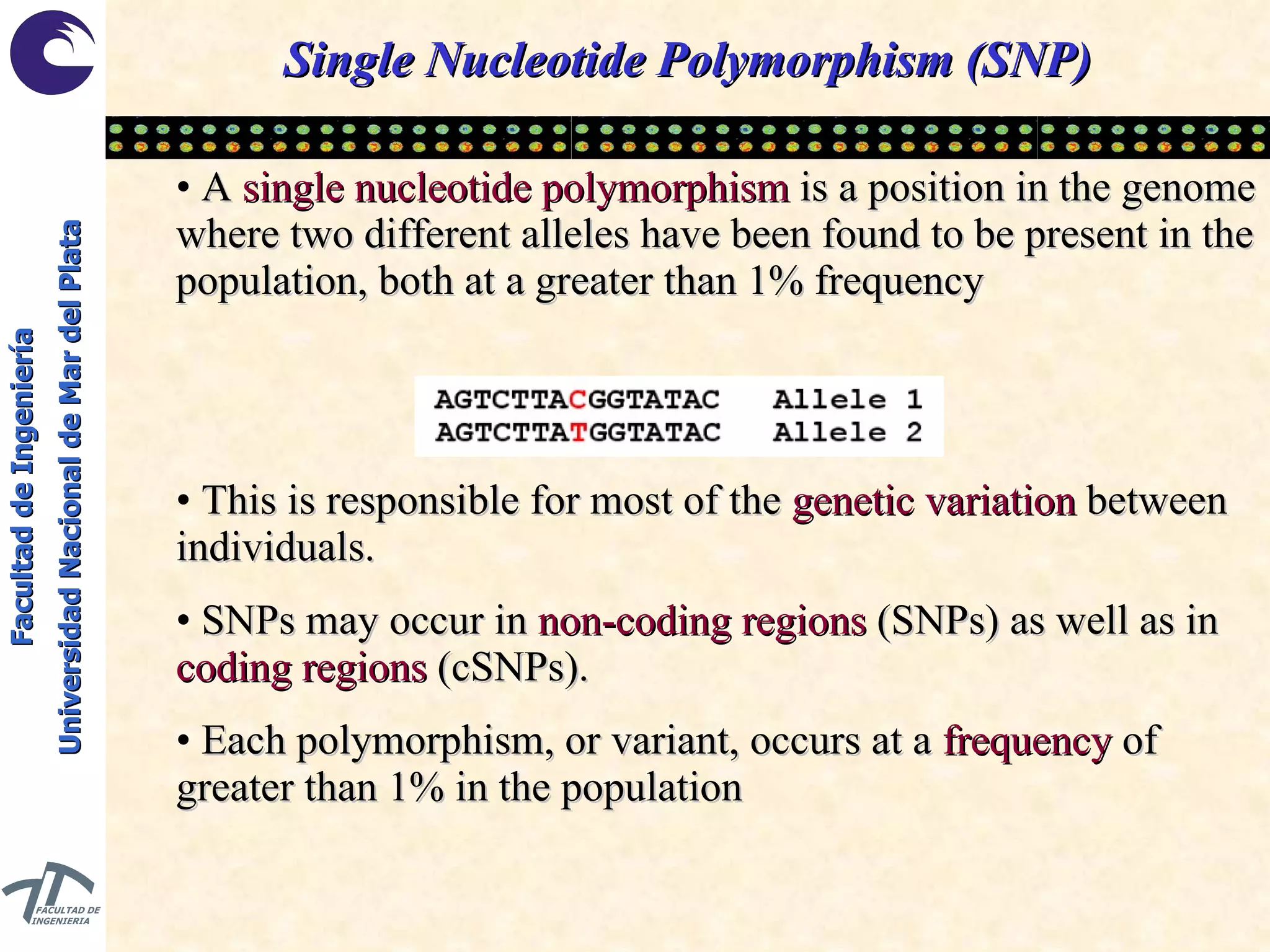

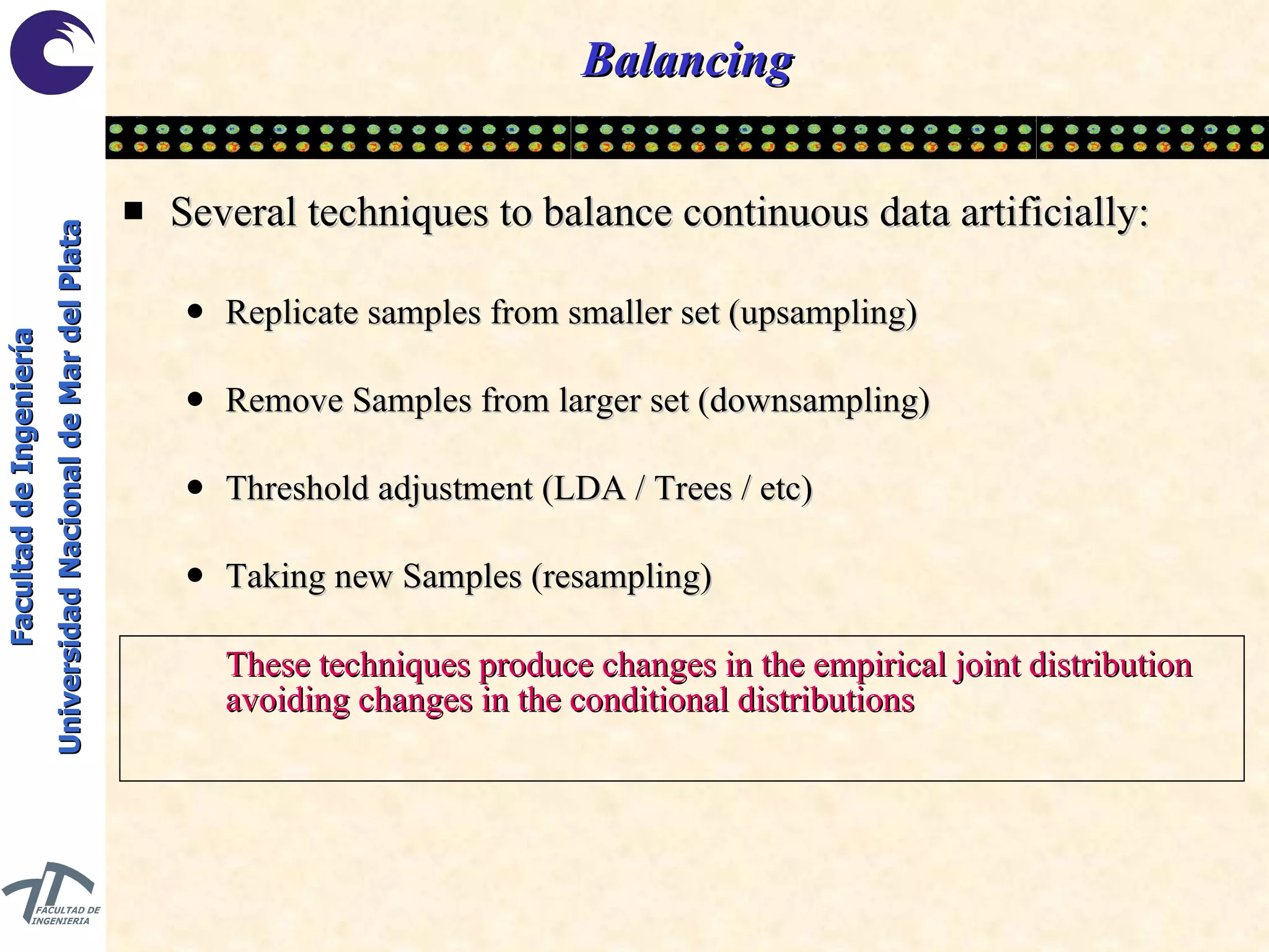
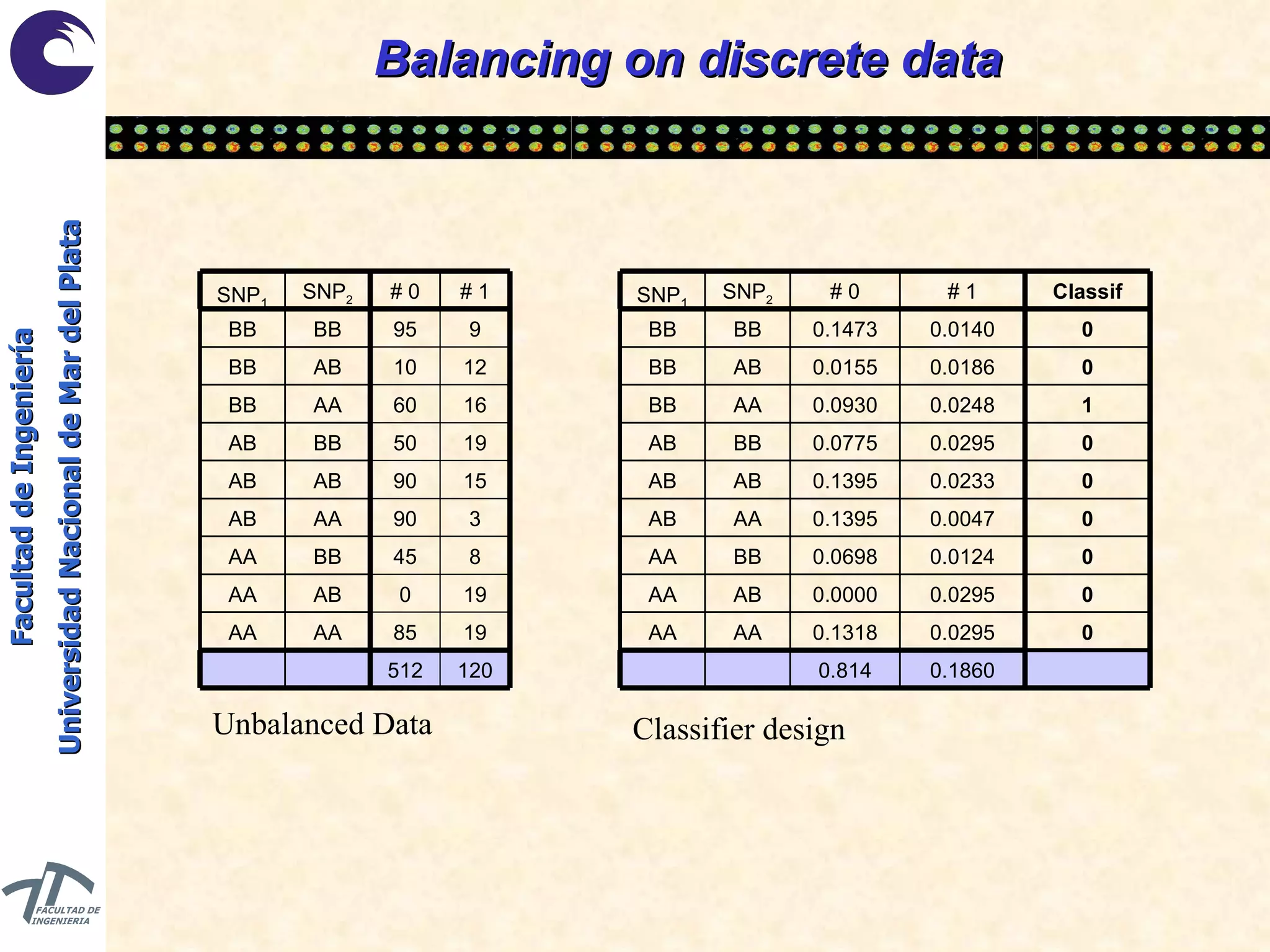
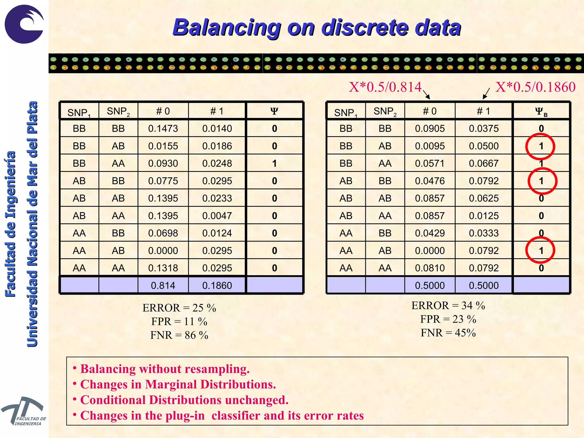
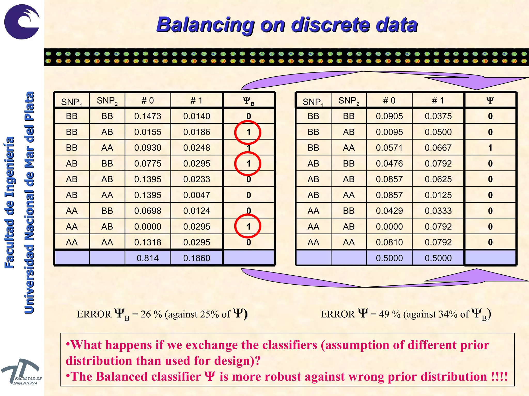
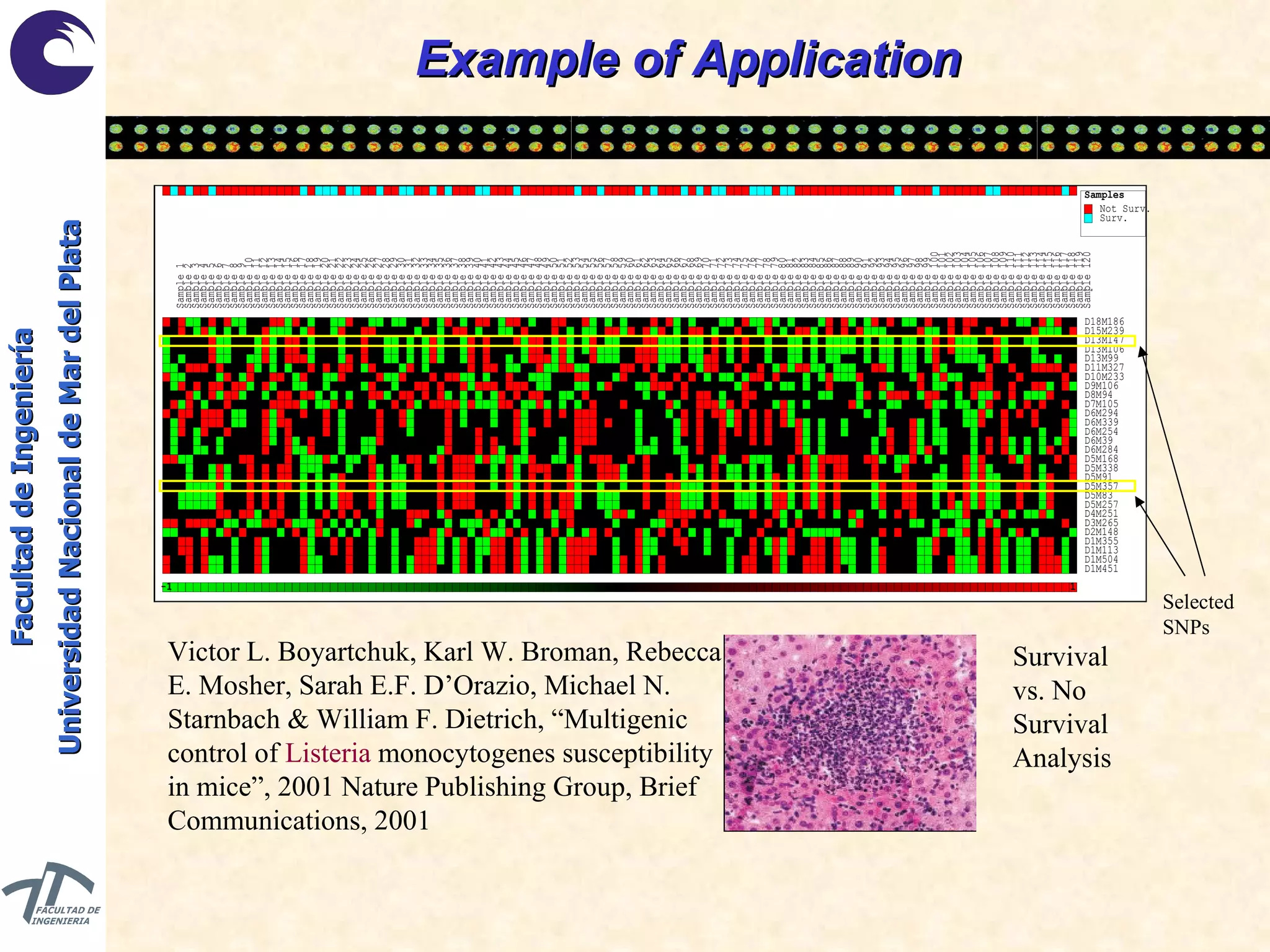
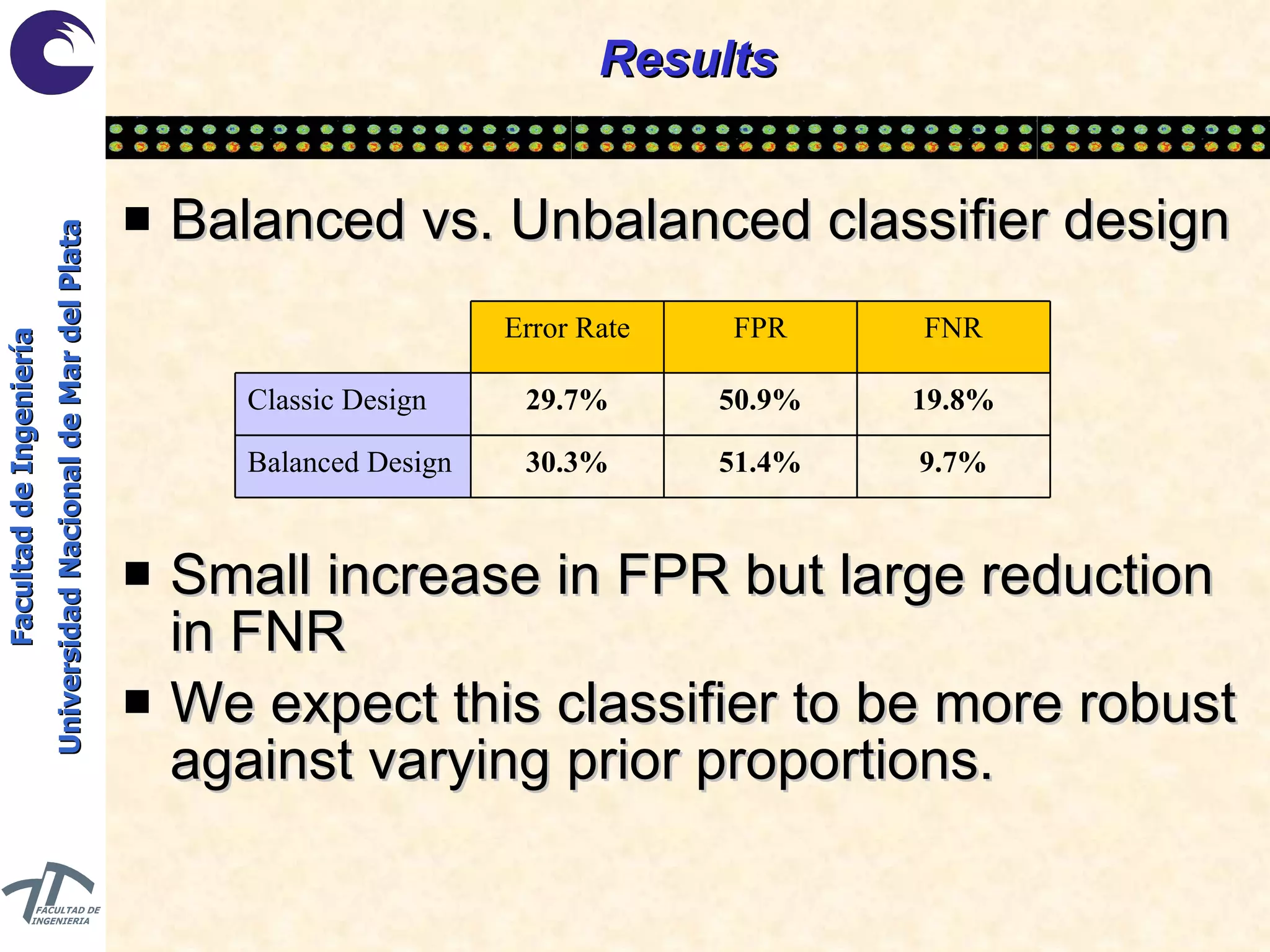
The document discusses balancing data for phenotype classification based on SNPs. It explains that training data often has imbalanced class distributions that do not reflect real-world proportions, affecting classifier design. Techniques are presented to balance discrete SNP data artificially by changing marginal distributions while keeping conditional distributions unchanged. This produces a classifier independent of sample proportions and more robust to incorrect prior assumptions. Balancing allows generating the same optimal classifier from any sample sizes.