
Recommended
Recommended
More Related Content
Similar to BEP342 CHAPTER 6 Critiques of Moneta
Similar to BEP342 CHAPTER 6 Critiques of Moneta (20)
More from ChantellPantoja184
More from ChantellPantoja184 (20)
Recently uploaded
Recently uploaded (20)
BEP342 CHAPTER 6 Critiques of Moneta
- 1. BEP342 CHAPTER 6 Critiques of Monetary Policy From Money and Banking: An Intermediate Market-Based Approach By William D. Gerdes (A Business Expert Press Book) Copyright © Business Expert Press, LLC, 2017. All rights reserved. Harvard Business Publishing distributes in digital form the individual chapters from a wide selection of books on business from publishers including Harvard Business Press and numerous other companies. To order copies or request permission to reproduce materials, call 1-800-545-7685 or go to http://www.hbsp.harvard.edu. No part of this publication may
- 2. be reproduced, stored in a retrieval system, used in a spreadsheet, or transmitted in any form or by any means – electronic, mechanical, photocopying, recording, or otherwise – without the permission of Harvard Business Publishing, which is an affiliate of Harvard Business School. This document is authorized for use only in DR. MD. SHAHIN MIA's FINANCIAL MARKETS AND INSTITUTIONS at Universiti Utara Malaysia from Apr 2021 to Oct 2021. http://www.hbsp.harvard.edu/ http://www.hbsp.harvard.edu CHAPTER 6 Critiques of Monetary Policy Critiques of Monetary Policy Fiat money is a relatively new phenomenon. It has been in use slightly more than three-quarters of one century. Tus, how historians will even- tually evaluate this experiment with fat money is yet to be determined. It is probably an understatement to suggest that the U.S. experience with this type of money, to this point, has not been an unmitigated success. Because fat monies are controlled by governments, what historians must eventually assess is how governments have performed.
- 3. Monetary policy is reasonably transparent and the performance of governments as custodians of fat money has not gone unnoticed. Te critiques discussed in the next sections are not concerned with situations where seigniorage is the principal motive of monetary authorities. Rather, the focus is on the practice of discretionary monetary policy in countries where macroeconomic management is the driving force behind policy. A common thread in critiques of monetary policy is the critical role that knowledge plays in the successful implementati on of discretionary mon- etary policy. Te critiques that follow demonstrate the multi - dimensional nature of the knowledge issue. One very important kind of knowledge required of central bankers is knowledge about the performance of the economy, somethi ng that is necessary if monetary authorities are to know whether monetary ease or tighter money is the appropriate policy. When knowledge does exist, it is not always apparent that central bankers will be in a position to utilize that knowledge. Political considerations may interfere. Central banks are also expected to understand how the policy they enact is transmitted to
- 4. the economy, and how those afected will respond to that policy. Finally, it is important for central banks to know what efect, if any, the infusion of new money has on relative prices and the allocation of resources across markets. This document is authorized for use only in DR. MD. SHAHIN MIA's FINANCIAL MARKETS AND INSTITUTIONS at Universiti Utara Malaysia from Apr 2021 to Oct 2021. 112 MONEY AND BANKING: AN INTERMEDIATE MARKET-BASED APPROACH Friedman: Rules vs. Discretion Milton Friedman argued that the use of discretionary monetary policy has resulted in increased economic instability. Te problem is not with the use of fat money. Rather, it is with the procedures employed by central banks to implement monetary policy, specifcally the use of discretionary policy. Replacing that type of policy with a monetary rule would greatly reduce economic uncertainty, especially uncertainty about the future course of monetary policy. Tis would provide a much better climate for produc-
- 5. tive activity and eliminate much of the economic instability occasioned by the use of fat money. In fashioning this position, Friedman’s posture is diametrically opposed to those who favor the use of discretionary policy. Proponents of discretionary policy maintain that its use can greatly improve macroeco- nomic performance. Appropriate application of policy instruments will both reduce short-run business cycle fuctuations and bring us greater long-run price stability. Monetary stimulation during a recession, for example, will shorten the recession. If too much infation is the problem, tighter monetary policy is in order. Friedman’s case against discretionary policy is that those implement- ing such policies most often do the wrong thing. Two principal reasons for this are: 1) politics, and 2) ignorance. By doing the wrong thing, those implementing discretionary policies make economic conditions worse rather than better. Politics Economic analysis of monetary policy often proceeds as if this policy were conducted in a political vacuum. Tat decidedly is not the case. Monetary policy is carried out by government, and the political
- 6. consequences of a policy action receive careful consideration. What is considered ratio- nal policy from a political perspective can difer signifcantly from that implied by economic theory. If political considerations dominate, those implementing discretionary policy may, with good reason, deliberately select the incorrect economic policy. Political considerations can afect monetary policy even in countries (such as the United States) that have a fairly independent central bank. When, for example, is a good time for the central bank to invoke a tighter This document is authorized for use only in DR. MD. SHAHIN MIA's FINANCIAL MARKETS AND INSTITUTIONS at Universiti Utara Malaysia from Apr 2021 to Oct 2021. CRITIqUES OF MONETARY POLICY 113 monetary policy that results in higher nominal interest rates? From a political perspective, the likely answer is never. As a consequence, central bankers bold enough to undertake such policies can expect politicians to sharply criticize their actions. Tat may be enough for policymakers contemplating such action to reconsider.
- 7. Elections cycles also create problems for those implementing discre- tionary monetary policy. In the absence of political pressure, introducing a policy change too close to an election can be interpreted as politically motivated. For central bankers in democratic countries who are sensitive to such charges, this might inhibit the implementation of an otherwise appropriate change in monetary policy. A second way that election cycles infuence monetary policy is through the actions of politicians concerned about an imminent election. Tey might exert pressure on central bankers to undertake policies favorable to their election (or reelection). Research suggests that, in the United States, this may be the rule rather than the exception. For the period from 1951 to the end of the 1970s, Robert Weintraub found that changes in Presi- dential administrations generally resulted in changes in monetary policy in a direction consistent with the economic views of the President.1 Given that Ronald Regan ran on a platform of reducing infation, Paul Volker’s disinfationary policies in the 1980s are an indication that Weintraub’s results extend beyond his sample period. A prototypical case study in central bank accommodation was
- 8. President Richard Nixon’s reelection campaign in 1972. Infation was increasing at the time, and economic theory implied a tighter monetary policy. Tighter money, however, was not the policy of choice for President Nixon. From his perspective, such policies had cost him the Presiden- tial election in 1960. He was not interested in a repeat of that experi- ence. Federal Reserve Chairman Arthur Burns accommodated President Nixon’s desire that monetary policy not be tightened. Nixon won the election, but at a considerable cost to the economy. Ignorance A second reason for the failure of discretionary policies is ignorance. Te existence of time lags presents a major problem for those attempting to implement discretionary policies. Tese lags imply that policy carried out This document is authorized for use only in DR. MD. SHAHIN MIA's FINANCIAL MARKETS AND INSTITUTIONS at Universiti Utara Malaysia from Apr 2021 to Oct 2021.
- 9. 114 MONEY AND BANKING: AN INTERMEDIATE MARKET-BASED APPROACH today has its impact in the future. Selection of the appropriate policy, then, requires the ability to forecast accurately. Economists, however, are notoriously weak when it comes to forecasting future economic activity. Tis ignorance is especially pronounced for turning points in the econ- omy, where one would anticipate signifcant changes in discretionary policy. Tree time lags encountered when implementing discretionary policy are the recognition lag, the execution lag, and the impact lag. To illustrate the difculties introduced by these time lags, refer to Figure 6.1. Real GDP (y) is plotted against time (t). Te business cycle peak occurs at time t1, with GDP equal to y1. Te decline in economic activity commencing at time t1 is not discov- ered until time t2. One reason for this lag is that published economic data generally are a record of the past, and turning points in economic activity often are not discovered in these data until well after they happen. For this cycle, the time interval (t2 – t1) is the recognition lag. It is the time that elapses between when the economy changes, and when
- 10. policy makers know about the change. Te policy response is not instantaneous. In the case of monetary pol- icy, the central bank must both adopt a new policy and implement that policy. Tese events too, require time. Assume that the policy response, which is additional monetary stimulation, occurs at time t3. Te time interval (t3 – t2), then, is the execution lag. Tis is the amount time that elapses between recognition of the problem and when policy makers undertake appropriate policy action. y y1 y0 y2 y3 y4 t0 t1 t2 t3 t4 t Figure 6.1 Discretionary policy with time lags This document is authorized for use only in DR. MD. SHAHIN MIA's FINANCIAL MARKETS AND INSTITUTIONS at Universiti Utara Malaysia from Apr 2021 to Oct 2021.
- 11. CRITIqUES OF MONETARY POLICY 115 Te impact of this policy action, likewise, is not instantaneous. Rather than occurring at a point in time, it is distributed over a period of time. Te precise timing of the impact is unknown. Friedman’s estimates for the U.S. economy are that it will have little (or no) impact for the frst 9–12 months, with the total impact occurring over a period of years. Simplifying, assume that the impact of monetary policy does occur at a single point in time (t4). By that time, the economy has already entered the expansionary phase of the business cycle. To moderate business cycle fuctuations, this phase of the cycle calls for monetary restraint. Instead of monetary restraint, however, the central bank is providing monetary stimulus. It has done the wrong thing. Monetary policy will accentuate the business cycle upswing and, in doing so, it increases the amplitude of the business cycle. Given the existence of these time lags, appropriate discretionary pol- icy for this economic cycle requires that the central bank undertake sim- ulative policy before the business cycle downturn occurs, e.g.,
- 12. at time t0. Te wisdom to do so, however, requires that (central bank) economists correctly forecast the impending peak at t1. Teir inability to accurately forecast turning points, or ignorance, generally precludes that. Friedman’s x-Percent Money Growth Rule Even though it is inadvertent, central bank implementation of discre- tionary monetary policy often makes things worse rather than better. For that reason, Friedman recommended scrapping discretionary policy. In its place, the central bank should follow a rule and increase the money supply at a constant rate. If, for example, a rate of 4% is selected, the central bank increases the money supply 4% each year. Tat is Friedman’s x-percent money growth rule. Te particular growth rate that is selected is less important than select- ing one. A rate in the neighborhood of 4% may be desirable, however, because it approximates the secular growth rate for production. Synchro- nizing the growth of money and output would permit (proximate) long- run price stability. Friedman maintains that the potential benefts of employing a monetary growth rule are enormous. Te principal one is a more stable
- 13. This document is authorized for use only in DR. MD. SHAHIN MIA's FINANCIAL MARKETS AND INSTITUTIONS at Universiti Utara Malaysia from Apr 2021 to Oct 2021. 116 MONEY AND BANKING: AN INTERMEDIATE MARKET-BASED APPROACH economy. A volatile monetary policy contributes to economic instability, thus increasing the amplitude of the business cycle. Use of a monetary rule efectively eliminates this source of cyclical instability. A second beneft is increased long-run economic growth. As mone- tary policy becomes more predictable, the uncertainty faced by those in private business is greatly diminished. Tis lowers the risk premium in interest rates, and will increase the rate of capital formation in the econ- omy. More capital formation leads to increased worker productivity and higher living standards. Finally, use of a monetary rule will eliminate of secular infation. Had the Federal Reserve employed such a rule in the past half- century, the great
- 14. depreciation that occurred in the purchasing power of the U.S. dollar would have been avoided. Elimination of secular infation will enhance the ser- vices provided by money, especially those eroded by unremitting infation. Despite these potential benefts, Friedman is aware of the forces militating against adoption of a monetary rule. A major force is the spir- itual legacy of the Enlightenment. Te great scientifc and economic achievements of the past several centuries have nurtured the sense that man has the ability to make things better through manipulation and con- trol. When placed in a monetary context, this perspective makes it easier for central bankers to inspire confdence in their ability to successfully manage monetary afairs. Public confdence in central bank stewardship is reinforced by central bank resistance to a monetary rule. Given the complexities of a modern economy, central bankers are often given much greater credit for their ability to manipulate aggregate economic activity than is warranted by experience. Te general public often basks in the comfort of a central bank that is “in control.” As human beings, it is natural that central bank- ers fnd such deference to their skills and infuence quite fattering. It is
- 15. contrary to human nature to expect them to embrace the prospect of replacing their reasoned judgments with a mechanical procedure that greatly diminishes their social signifcance. The Road Not Taken: A Friedman Case Study It is not possible to know what would have happened had the Federal Reserve followed Friedman’s x-percent money growth rule. Tat is a road This document is authorized for use only in DR. MD. SHAHIN MIA's FINANCIAL MARKETS AND INSTITUTIONS at Universiti Utara Malaysia from Apr 2021 to Oct 2021. CRITIqUES OF MONETARY POLICY 117 Table 6.1 Dynamic Equation of Exchange for the U.S. Economy (Average Annual Growth Rate: 1959–2015) dM/M + dV/V = dP/P + dy/y Actual U.S. data 6.9 -0.4 3.4 3.1 Data with x-percent money growth 4.0 -0.4 -0.5 4.1
- 16. Source: U.S. Department of Commerce, www.bea/gov (retrieved 10/24/2016), and U.S. Govern- ment Printing Offce, Economic Report of the President (various issues), www.presidency/ucsb/ edu/economic_reports (retrieved 10/24/2016). not taken. It is possible, however, to simulate what Friedman had in mind through the prism of the dynamic version of the equation of exchange. In Table 6.1, that relationship is utilized to compare actual data for the 56-year period from 1959–2015 with hypothesized data using Friedman’s x-percent growth rule. From 1959–2015, annual U.S. money growth (dM2/M2) averaged 6.9%. Long-run velocity was relatively stable, declining at an average annual rate of 0.4%. Real Gross Domestic Product growth (dy/y) averaged 3.1%. With too much money chasing too few goods, the United States experienced an average secular infation rate (dP/P) of 3.4% per year. By comparison, assume the Federal Reserve implements Friedman’s x-percent growth rule by increasing the money supply by 4% each year. Te velocity of money is relatively stable with the assumed annual growth rate (dV/V) the same as the actual growth rate for 1959–2015: – 0.4%. Friedman argued that such monetary stability would lead to
- 17. higher eco- nomic growth. Accordingly, the average annual growth rate for real GDP is 4.1%. Tat was the actual rate of growth for the 1950s, the decade prior to the implementation of Keynesian economic policies during the J.F. Kennedy administration. For the period under consideration, Friedman’s x-percent money growth rule yielded long-run price stability. Prices, on average, declined 0.5% per year. Such price stability is comparable to that experienced by the United States when the country was using fduciary money (prior to 1933). Had the United States actually experienced such price stability, the considerable erosion in the services provided by money would probably not have occurred. For example, with long-run price stability, money would have continued to serve as a viable store of value. In addition, Friedman would likely make the case that United States would have been spared the dislocations and economic hardships associated with the This document is authorized for use only in DR. MD. SHAHIN MIA's FINANCIAL MARKETS AND INSTITUTIONS at Universiti Utara Malaysia from Apr 2021 to Oct 2021. www.presidency/ucsb
- 18. www.bea/gov 118 MONEY AND BANKING: AN INTERMEDIATE MARKET-BASED APPROACH Great Infation of the 1970s and the ensuing disinfation of the 1980s. He also might argue that, with the x-percent money growth rule, the United States would not have sufered through the Great Recession of 2008–2009. A policy of providing new money at a steady rate (instead of pushing short-term interest rates close to zero for an extended period) would reduce the likelihood of an asset bubble in housing that was at the epicenter of the Great Recession. Interest Rate Targeting Central banks in relatively advanced countries generally employ inter- est rate targeting to implement discretionary monetary policy. Excluding the four-year interlude from 1979–1983, the Federal Reserve System in the United States has targeted interest rates for several decades. While the analysis that follows applies to interest rate targeting more generally, the issue is framed within the context of U.S. monetary policy. Federal Reserve interest rate targeting conforms to the transmission
- 19. mechanism described as Model I in the previous chapter. Te instrument variable is open market operations (OMO). Te immediate target is the short-term interest rate (ist). Te rate selected for this purpose is the fed- eral funds rate, or the rate on immediately available funds. While it is a nominal interest rate, the intermediate target is the long-term real interest rate (rlt). Te ultimate policy objectives are the price level and aggregate spending. Te Fed encounters two very difcult problems when attempting to implement policy through this transmission mechanism. First, it is using a nominal interest rate target in a world where rational economic agents think in real terms. Te interest rate of importance, then, is the unobserv- able real interest rate. Second, the transmission of monetary policy occurs across the term structure of interest rates. Te immediate target is a short- term interest rate, but the critical variable is the long-term rate of interest. The Nominal/Real Dichotomy Te success of Federal Reserve monetary policy is contingent upon con- trol of the real interest rate. Rational economic agents on both sides of the
- 20. This document is authorized for use only in DR. MD. SHAHIN MIA's FINANCIAL MARKETS AND INSTITUTIONS at Universiti Utara Malaysia from Apr 2021 to Oct 2021. CRITIqUES OF MONETARY POLICY 119 credit market think in real terms and, if one is to change their behavior through policy, it is the real interest rate that counts. Unlike the nominal interest rate, however, the real interest rate is unobservable. Te difculty presented here is that one cannot readily control something that does not lend itself to measurement. Tat problem is compounded when preci- sion is required. Tat is generally the case, however, because policymakers employing nominal immediate targets most often change those interest rate targets in increments of one-quarter to one-half percent. Control of the unobservable real rate of interest is hypothesized to occur via changes in the Federal Reserve’s nominal interest rate target (the federal funds rate). As noted in Chapter 3, however, the nominal rate of interest, too, is comprised of nonobservable components: infation-
- 21. ary expectations; default, money, and income risk premiums; and, time preferences. Each of these components refects the subjective valuations of millions of market participants. Because subjective valuations of indi- vidual economic agents are prone to change, one must operate on the premise that they do. Tat is, infationary expectations, risk premiums, and time preferences are incessantly changing. If these nonobservable components of the nominal rate of interest are unstable, when the Fed changes its nominal interest rate target, it cannot know whether the real interest rate is increasing, falling, or staying the same. If a policy-induced higher real interest rate indicates a tighter monetary policy, and a policy-induced lower real rate the opposite, the Federal Reserve does not know whether its monetary policy is tighter, easier, or neutral. To illustrate, three diferent scenarios are presented in Table 6.2. Tey are designated as Cases I, II, and III. Te frst scenario (Case I) is the initial condition. Te nominal interest rate is 5%, which is also the Fed’s targeted interest rate. With a 2% expected rate of infation, the real Table 6.2 The Nominal Interest Rate and Its Components
- 22. i r (dp/p)* Risk premium Marginal rate of time preference Case I 5 3 2 ½ 2½ Case II 6 4 2 ½ 3½ Case III 4 2 2 ½ 1½ This document is authorized for use only in DR. MD. SHAHIN MIA's FINANCIAL MARKETS AND INSTITUTIONS at Universiti Utara Malaysia from Apr 2021 to Oct 2021. 120 MONEY AND BANKING: AN INTERMEDIATE MARKET-BASED APPROACH interest rate is 3%. Te latter is apportioned into a risk premium and a marginal rate of time preference.2 Assume, initially, that the Federal Reserve attempts to tighten mon- etary policy. In Case II, it raises its target for the nominal interest rate to 6%, and provides reserves less liberally to the banking system. With tighter credit conditions, the nominal rate increases to the desired level. Assuming no change in infationary expectations, the real rate increases to
- 23. 4%. Te higher real rate of interest leads to reduced capital goods expen- ditures, and a higher marginal rate of time preference. In this scenario, the Fed thinks that monetary policy is tighter and, indeed, it is. Tis is how monetary policy with interest rate targeting is supposed to work. With the subjective preferences of economic agents constantly chang- ing, however, the world is much more complex than this. For example, do these Case II numbers still constitute tighter monetary policy if the higher real interest rate would have occurred as a result of market activity alone? Commence again with Case I initial conditions, i.e., i = 5% and r = 3%. Now, assume an increasingly robust economy with businessmen becoming more optimistic. Teir increased time preferences for current expenditures are expressed in the form of a greater demand for capital goods. Tighter credit conditions lead to a higher nominal rate (6%) and a higher real rate (4%). Case II numbers again prevail. Superimpose upon these events an increase in the Federal Reserve’s target for the nominal interest rate—from 5% to 6%. Te Fed’s objective is to increase the real interest rate by 1% (from 3% to 4%). In this case, the Fed does not need to adjust how it is providing reserves to
- 24. the bank- ing system. Te higher interest rates come about through market activity alone, and do not refect any change in Fed policy. When the Federal Reserve adjusts its interest-rate target upward, that target is simply fol- lowing the market rate. Tis is a case where the Federal Reserve thinks monetary policy is tighter when, in fact, it is not. Errors of this kind are likely when the real interest rate follows a pro-cyclical pattern. If business managers and consumers become more optimistic during a business cycle expansion, their greater optimism is expressed in the form of an increase in their time preferences for current expenditures. Te real (and nominal) interest rate rises. If the Federal Reserve simultaneously becomes concerned about the This document is authorized for use only in DR. MD. SHAHIN MIA's FINANCIAL MARKETS AND INSTITUTIONS at Universiti Utara Malaysia from Apr 2021 to Oct 2021. CRITIqUES OF MONETARY POLICY 121 exuberant economy, it will move to tighten monetary policy. As in the example above, however, it will erroneously interpret the
- 25. market-driven rise in interest rates as policy-induced. Te Federal Reserve is prone to making the opposite kind of error when the economy is contracting. Business managers and consumers become more pessimistic. Tey experience decreases in their time pref- erences for current expenditures, and the real (and nominal) interest rate falls. Te Fed, in an attempt to stimulate aggregate demand, lowers its interest rate target. With the nominal and real rate already falling, the Fed is unable to distinguish market-induced declines in rates from those occasioned by Fed policy. Tis scenario is captured in Case III (Table 6.2). Commencing with the initial condition (Case I), declines in the real and nominal rate occur in response to reduced time preferences. Te nominal rate falls from 5% to 4%; the real rate, from 3% to 2%. Simultaneously, the Federal Reserve lowers its target for the nominal interest rate from 5% to 4%. Its intent is to lower the real rate by a similar amount (from 3% to 2%). Te Federal Reserve does not need to adjust its provision of reserves to the banking system, because both the nominal and real rates reach their targeted levels through market activity. Tis is a case where the Fed thinks that
- 26. monetary policy is easier when, in fact, it is not. Tus, there are serious reservations concerning the Federal Reserve’s ability to efectively control the real rate of interest. When the Fed changes its nominal interest rate target, it does not know with any assurance either the magnitude or direction of policy-induced changes in the real rate of interest. The Term Structure Problem A second problem the Federal Reserve confronts when targeting interest rates relates to the term structure of interest rates. Not only does the Fed not know whether adjustments in its immediate target result in the desired change in the real interest rate, but those policy changes also must be transmitted across the term structure of interest rates. Te Federal Reserve’s operating target is the short-term nominal rate, but its interme- diate target is the long-term real interest rate.3 This document is authorized for use only in DR. MD. SHAHIN MIA's FINANCIAL MARKETS AND INSTITUTIONS at Universiti Utara Malaysia from Apr 2021 to Oct 2021.
- 27. 122 MONEY AND BANKING: AN INTERMEDIATE MARKET-BASED APPROACH Te rationale for this transmission mechanism (Model I) is discussed in Chapter 5. Outlays for durable goods, both business and consumer, are more easily deferred than are expenditures for nondurable goods. As a consequence, durable goods account for much of the volatility in aggre- gate spending. Attempts by policy makers to infuence aggregate spending (and the price level), then, are geared towards controlling expenditures for those types of goods. With durable goods purchases frequently fnanced through the issue of long-term bonds, those purchasing durable goods are sensitive to the long-term rate of interest. It follows that, when the Fed employs interest rate targeting, it must target the long-rate. Precisely how the Federal Reserve successfully navigates the term structure and, simultaneously engineers changes in the real interest rate, is not clear. Moreover, various theories of the term structure (discussed in Chapter 3) do not provide much help. If anything, they cast additional aspersion upon the Fed’s ability to successfully implement discretionary policy through interest-rate targeting. Explanations based on the segmented markets hypothesis, for
- 28. exam- ple, are not encouraging. If market participants adhere strongly to their maturity preferences, there is little likelihood that policy- induced changes in the short-term interest rate target will be transmitted across the term structure to long-term rates of interest. Federal Reserve control, in turn, is marginalized. On the other hand, information requirements implied under the unbiased expectations and the liquidity preference theories present an even more serious obstacle for those conducting monetary policy. First, the Fed must have prior knowledge of the term structure of infation pre- miums and the term structure of risk premiums. Second, it must know how those term structures are changing independent of monetary policy. Finally, it must also know how a given change in its short-term interest rate target will afect both of those underlying term structures. Com- pounding the Fed’s information problem is the fact that both infationary expectations and risk premiums are imbedded in the term structure of interest rates, and not directly observable. It is clear that the U.S. central bank faces serious information prob- lems when attempting to target long-term real interest rates through use
- 29. of a short-term nominal operating target. If the Federal Reserve acts as This document is authorized for use only in DR. MD. SHAHIN MIA's FINANCIAL MARKETS AND INSTITUTIONS at Universiti Utara Malaysia from Apr 2021 to Oct 2021. CRITIqUES OF MONETARY POLICY 123 if it can orchestrate desired changes in aggregate spending and the price level through this procedure, it is committing what Friedrich von Hayek called “the pretense of knowledge.”4 It is pretending to know things that, in fact, it does not. A Twenty-First Century Case Study Tis knowledge problem confronting the Federal Reserve is a good illus- tration of what happens when the criteria for selecting monetary targets (discussed in the previous chapter) are not satisfed. Because it is not pos- sible to accurately measure the long-term real interest rate, the Federal Reserve is employing a target it cannot control. Moreover, lack of knowl- edge of the long-term real rate also means the linkages in Model I are not
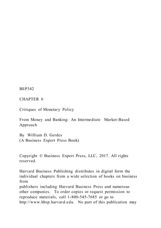
- 30. predictable. U.S. monetary policy from 2004–2006 exemplifes the difculties encountered when these monetary target criteria are not met. Starting in June, 2004, the Federal Reserve increased its target for the federal funds rate ffteen consecutive times. As a consequence, the federal funds rate target in April, 2006 was 4.75% versus 1.00% in the frst half of 2004. Tose changes are chronicled in Table 6.3. Many observers routinely describe these upward adjustments in the federal funds rate target as tighter monetary policy. Tere are seri- ous doubts, however, about such an interpretation. It is true that other short-term nominal rates increased along with the federal funds rate. Te three-month Treasury-bill rate, for example, rose from 1.17% to 4.60% between June 1, 2004 and March 1, 2006.5 But, as previously noted, higher short-term nominal interest rates do not necessarily mean tighter monetary policy. Long-term nominal interest rates actually fell during the same 21-month period. Te rate for 20-year U.S. Treasury securities declined from 5.45% to 4.74%. Tese changes in both long-term and short-term rates for U.S. Treasury securities are refected in Figure 6.2. It depicts the shapes of the term structure of inter-
- 31. est rates for U.S. Treasury securities on both June 1, 2004 and March 1, 2006. Te yield curve in 2006 became noticeably fatter. Lower long-term nominal interest rates, however, are not the issue. It is long-term real interest rates, and not nominal rates, that are critical for This document is authorized for use only in DR. MD. SHAHIN MIA's FINANCIAL MARKETS AND INSTITUTIONS at Universiti Utara Malaysia from Apr 2021 to Oct 2021. 124 MONEY AND BANKING: AN INTERMEDIATE MARKET-BASED APPROACH Table 6.3 Federal Funds Rate Target Date Level (percent) 2006 March 28 4.75 January 31 4.50 2005 December 13 4.25 November 01 4.00
- 32. September 20 3.75 August 09 3.50 June 30 3.25 May 03 3.00 March 22 2.75 February 02 2.50 2004 December 14 2.25 November 10 2.00 September 21 1.75 August 10 1.50 June 30 1.25 2003 June 25 1.00 Source: Board of Governors of the Federal Reserve System. 6 5 4 3
- 33. 2 1 0 3 month 6 month 1 year 5 year 10 year 20 year 6/1/2004 3/1/2006 Figure 6.2 Term structure of interest rates U.S. treasury securities: Constant maturity Source: Board of Governors of the Federal Reserve. This document is authorized for use only in DR. MD. SHAHIN MIA's FINANCIAL MARKETS AND INSTITUTIONS at Universiti Utara Malaysia from Apr 2021 to Oct 2021. CRITIqUES OF MONETARY POLICY 125 economic decision makers. If monetary policy was, indeed, tighter during this 21-month period, long-term real interest rates must have increased while nominal rates were falling. Moreover, the increase in real rates must have occurred as a result of monetary policy and not due to other factors such as an increase in default risk or changes in time
- 34. preferences for cur- rent expenditure. While such a scenario appears doubtful, no one knows for certain. Hence, the appropriate answer to the question about whether monetary policy is tighter is: “I don’t know.” Monetary Aggregates and Monetary Control Recent Issues with Monetary Control After facing difculties with interest-rate targeting during and after the Great Recession (2008–2009), the Federal Reserve embarked on sev- eral massive asset purchase programs described as quantitative easing. Tose carried out during the Great Recession are discussed in Chapter 5 (pp. 108–109). While the Fed’s asset purchase programs were not advanced with the stated intent of increasing monetary aggregates, they did. In doing so, these programs raised an additional issue relating to central bank control of the money supply. Tese issues are discussed in the context of the gen- eral money supply model in Chapter 4 (equation 4.2). Te magnitude of the Federal Reserve’s asset purchases caused the monetary base in the United States to explode. Base money increased more than 360% from 2007 and 2014, and was largely in the
- 35. form of increases in bank reserves. Under more normal circumstances, one would anticipate a massive increase in the money supply, huge increases in spending, and the potential for the largest infation in U.S. history. To date, none of these things have happened. Te reason is that banks have not used this infusion of bank reserves to extend additional bank credit (and expand deposit money). Instead, those reserves were almost entirely held in the form of excess reserves. In the money supply model, an increase in the aggregate bank excess reserve ratio causes the money multiplier to decrease. In this case, because the increase in bank excess reserves was so massive, the multiplier collapsed. This document is authorized for use only in DR. MD. SHAHIN MIA's FINANCIAL MARKETS AND INSTITUTIONS at Universiti Utara Malaysia from Apr 2021 to Oct 2021. 126 MONEY AND BANKING: AN INTERMEDIATE
- 36. MARKET-BASED APPROACH As shown in equation (6.1), the large increase in the monetary base was virtually entirely ofset by a fall in the money multiplier. In the con- text of these changes the consequences for money (which did rise) were minimal. M = B m. (6.1) ← ↑ ↓ Tis experience has important implications for monetary policy. It difers from the liquidity trap explanation advanced by early Keynesians. In that case, the central bank increases the money supply and it has no efect on spending. People hold rather than spend the additional money, and velocity falls. When this happens, monetary policy is inefective. In the present case, the efectiveness of monetary policy is questioned for a diferent reason. Unlike the previous case, the money supply does not increase, or it does so minimally. What distinguishes the recent expe- rience is collapse of the money multiplier as shown in (6.1). Te precipitous fall in the multiplier represents a breakdown in a transmission mechanism for monetary policy. In Chapter 5, the trans- mission mechanism employing monetary aggregates as targets
- 37. was Model II. In that transmission mechanism, what links base money to the money supply is the base money multiplier. Te usefulness of that transmission mechanism is predicated upon a predictable relationship for transforming base money into money. It is that relationship that fell apart. Tis experience raises serious questions concerning the ability of the Federal Reserve to control the money supply. When combined with the lackluster results from interest rate targeting, it appears that both trans- mission mechanisms I and II for implementing discretionary monetary policy did not perform as expected during and after the Great Recession (2008–2009). Why the Federal Reserve Needs an Exit Strategy Te massive infusion of bank reserves (and base money) into the U.S. fnancial system from 2008 to the present leaves the Federal Reserve with an important legacy issue. If the United States is to avoid signifcant This document is authorized for use only in DR. MD. SHAHIN MIA's FINANCIAL MARKETS AND INSTITUTIONS at Universiti Utara Malaysia from Apr 2021 to Oct 2021.
- 38. CRITIqUES OF MONETARY POLICY 127 future infation, the Fed must undertake future monetary policy that (largely) removes that base money from the system or, alternatively, pro- vides banks with an incentive to not activate the massive excess reserves they now hold. Te description of how the Federal Reserve plans to do this is known as the Fed’s exit strategy. Te magnitude of the problem confronting the Federal Reserve is apparent in Table 6.4. From 2007–2014, bank reserves and base money increased by 2,813% and 364%, respectively. Tese dramatic increases were not refected in the money supply (M2) which rose by only 56.4%. Tis surprisingly modest number is the result of the collapse of the base money multiplier (m), which fell by 64.4%. Tese data comport with the directional changes in equation (6.1) above. Te problem confronting the Federal Reserve is about what happens if banks activate available excess reserves. Since the most recent business cycle trough (June, 2009), businesses and households have behaved very cautiously. Credit demands by both sectors have been restrained, and
- 39. economic growth has been tepid. Table 6.4 Bank Reserves, Base Money, Money Supply, and the Money Multiplier for the United States 2001–2014 Year Reserves Base money M2 m 2001 86.3 641.1 5181.7 8.08 2002 88.1 697.1 5565.8 7.98 2003 93.4 741.0 5953.5 8.03 2004 96.3 776.8 6235.5 8.03 2005 96.7 806.6 6501.8 8.06 2006 95.0 835.0 6842.9 8.20 2007 93.9 850.5 7263.1 8.54 2008 234.9 835 7757.5 7.67 2009 945.2 1796.8 8383.0 4.67 2010 1143.4 2031.7 8593.4 4.23 2011 1575.7 2539.1 9224.7 3.63 2012 1612.0 2662.2 10020.0 3.76 2013 2144.2 3271.8 10696.4 3.27 2014 2735.4 3947.0 11356.8 2.88 Source: St. Louis Federal Reserve Bank-FRED (//fred.stlouisfed.org), October 31, 2016.
- 40. This document is authorized for use only in DR. MD. SHAHIN MIA's FINANCIAL MARKETS AND INSTITUTIONS at Universiti Utara Malaysia from Apr 2021 to Oct 2021. https://fred.stlouisfed.org 128 MONEY AND BANKING: AN INTERMEDIATE MARKET-BASED APPROACH If, in the future, both businesses and households throw caution to the wind, and become very aggressive in their demands for credit, banks (which are awash in liquidity) are in a position to accommodate them. Moreover, banking competition makes them inclined to do so. If an indi- vidual bank refuses a customer’s demand for credit, that customer is likely to take his/her banking business to another bank. Meeting these credit demands means an increase in money growth, which has the potential to accelerate sharply. Te acceleration in money growth, in this case, is occasioned by an increase in the base money mul- tiplier. As banks reduce their holdings of excess reserves, the aggregate excess-reserve ratio falls and the money multiplier rises.
- 41. Te potential impact on the money supply is captured by assuming that the multiplier returns to its prerecession level of 8.54 (2007). If that adjustment had occurred in 2014, the impact on the money supply for that year is shown in (6.2). M2 = $33,707.4 = B = $3,947.0 * 8.54 (6.2)2014 * m2007 With a multiplier of 8.54 in 2014 (and assuming the same 2014 level for base money), the money supply would have been $33,707.4 billion for that year instead of the recorded level of $11,356.8 billion. Tat represents a 196.8% increase in the money supply. In other words, the money supply has the potential to grow this much if the multiplier were to return to its prerecession level. If all of this money growth were to occur in a single year, the average price would increase by a magnitude of the same order, or 196.8%.6 Tus, the potential exists for the highest infation rates in U.S. history. Tat is why the Federal Reserve needs an exit strategy. Rational Expectations Economists know that a person’s expectations afect the economic deci- sions made by that individual. Rational expectations theory is concerned with how those expectations are formed and, also, how
- 42. economists model those expectations. Much of this theory was developed in response to the This document is authorized for use only in DR. MD. SHAHIN MIA's FINANCIAL MARKETS AND INSTITUTIONS at Universiti Utara Malaysia from Apr 2021 to Oct 2021. CRITIqUES OF MONETARY POLICY 129 use of large macroeconometric models (by business and government). Sta- tistical in form, these models were an adjunct to the Keynesian revolution in macroeconomic theory. Te models often contained several hundred equations, and were used for forecasting purposes. Keynesian economists used the models to advise governments about the consequences of difer- ent activist policies, while those in the private sector used them as an aid in business decision-making. Many of the equations in macroeconometric models were behavioral in nature. Tat necessitated the modeling of expectations, even though those expectations were unobservable. Proxies for these unknown expec- tations were most often obtained by assuming that economic agents have adaptive expectations. With this approach, the expected value of
- 43. a vari- able was estimated as a weighted sum of past values of that same vari- able. Historical time series data were employed for rendering concrete estimates. Econometric models constructed using this methodology often result in large forecasting errors, and economists in the rational expectations tradition have a ready explanation for this. Reliance on adaptive expec- tations as a proxy for actual expectations is an inherent weakness of the models. For, modeling human behavior in this way is tantamount to assuming that economic agents are irrational. Te reason is that economic agents with adaptive expectations make systematic errors. Tat is, they repeatedly make the same mistakes. An alternative to assuming that expectations are adaptive is to assume they are rational. Rational individuals are not restricted to using past information (such as past values of variables) when forming their expec- tations. Teir expectations are formed by taking into account all informa- tion that is worthwhile acquiring. Agents behaving in this fashion are said to have rational expectations. Once the models of economists incorporate rational expectations, economic agents are less prone to making
- 44. the same mistakes repeatedly—systematic errors. Moreover, such rational behavior has implications for the efectiveness of economic policy. If economic policy afects economic agents in a signifcant way, then it is rational for them to take the efects of that policy into account. Further- more, if those administering policy behave consistently, economic agents will learn how that policy is implemented under diferent economic This document is authorized for use only in DR. MD. SHAHIN MIA's FINANCIAL MARKETS AND INSTITUTIONS at Universiti Utara Malaysia from Apr 2021 to Oct 2021. 130 MONEY AND BANKING: AN INTERMEDIATE MARKET-BASED APPROACH Table 6.5 Policy Impotence Theorem Period M V = P y I → ↑ → ↑ II ↑ ↓ → → circumstances. Once they do, individuals will adjust their behavior to the policy, and make necessary behavioral changes before any
- 45. change in policy is undertaken. Because adjustment to the policy has already taken place, no behavioral response follows any predictable change in economic policy. In rational expectations theory, this result is known as the Policy Impotence Teorem. When behavior is rational in this sense, discretionary policy loses its efectiveness. An example of such policy impotence in the context of ratio- nal economic behavior is chronicled in Table 6.5. In Period I, individuals anticipate monetary ease that will occur in Period II. Sensing that they will be able to fnance additional expenditures at a lower rate in the near future, they adjust their current expenditures upward. Producers respond by increasing production in Period I and, in the absence of a change in the money supply, the ofsetting entry in the equation of exchange is an increase in the velocity of circulation of money (V↑). In period II, the central bank increases the money supply to stimu- late aggregate demand. However, there is no increase in spending because rational economic agents anticipated this monetary stimulation and have already adjusted their spending plans (in Period I). In Table 6.5, the money supply increases in Period II but GDP expenditures
- 46. remain the same. Te ofsetting entry is a decline in velocity (V↓). Te monetary ease engineered by the central bank in Period II has no efect on current spending, i.e., it was impotent. Te rational expectations argument against the use of discretionary policy does difer from that of Friedman (and the monetarists) in one important respect. In Friedman’s case, discretionary policy does not work because policymakers are either ignorant or subject to political infuence. For the rational expectations economists, discretionary policy does not work because those afected by the policy are the opposite of ignorant. Tey are too smart (or rational). This document is authorized for use only in DR. MD. SHAHIN MIA's FINANCIAL MARKETS AND INSTITUTIONS at Universiti Utara Malaysia from Apr 2021 to Oct 2021. CRITIqUES OF MONETARY POLICY 131 The Austrian Perspective on Monetary Policy
- 47. Economists in the Austrian tradition generally favor “hard money.” Tey fnd it vexing that a monetary economist such as Milton Friedman favors reliance upon markets everywhere except in his area of expertise, the realm of money. Te Austrian position is that money is too important to be left to government. Instead, money and all monetary relations should be determined through exchange activities in the marketplace. Because fdu- ciary money was a spontaneous market development, and fat money was not, Austrians generally favor reestablishing fduciary money by returning to the gold standard. If the quantity of money and all monetary relations are determined by market participants, government has no monetary role. Tere is no monetary policy. For that reason, Austrians are against all monetary pol- icy as practiced under fat money regimes. Tat would include Friedman’s monetary growth rule as well as all variations of discretionary policy. At the center of the Austrian critique of monetary policy is the con- cept of the price level. Te importance attached to the idea of an average price dates back to the early 20th century, when Irving Fisher argued that the value of money should be standardized.7 By this, he meant
- 48. that the objective of government monetary policy should be to stabilize the average price, or the price level. While Fisher was unsuccessful in his crusade to standardize money, the concept of the price level subsequently assumed a life of its own. After governments mandated the use of fat money, the price level became a variable subject to manipulation by monetary authorities. Despite the eforts by central banks to manage the price level, Austrians give the concept little credence. For them, the price level has no signifcance independent of its component parts—the individual prices. To the extent that there is an average price, it is an aggregation of these individual prices. In a market setting, each individual price has meaning, or informational content. Each is an expression of the subjective valua- tion that individuals have placed on that object. Viewed collectively, a set of individual prices represents relative valuations. With no rigid dichotomy separating microeconomics and macro- economics, the signifcance Austrians attach to individual prices is not restricted to the realm of microeconomics. Tey are equally important This document is authorized for use only in DR. MD. SHAHIN MIA's FINANCIAL MARKETS AND INSTITUTIONS at Universiti Utara Malaysia from
- 49. Apr 2021 to Oct 2021. 132 MONEY AND BANKING: AN INTERMEDIATE MARKET-BASED APPROACH in a macroeconomic setting. Hence, when central banks manipulate the price level, without regard to its constituent parts, they destroy the infor- mational content of individual prices. In doing so, they disrupt the crit- ical role that prices play in coordinating the diverse economic activities that collectively make up the aggregate economy. Assume, for example, that a central bank employs monetary policy to stabilize the average price. Te problem here is that market participants may have preferences that are not consistent with an unchanged exchange value for money. In the absence of monetary policy, they may have valued money either more highly or less highly than before. If they valued money more highly, their preferences were consistent with defation rather than price stability. Alternativel y, placing a lower value on money would result in infation. When money is a strictly a market phenomenon, infation, defation, and price stability are all possible outcomes. Moreover, there is
- 50. no analyt- ical basis for favoring one of these outcomes over the others. Tis view is antithetical to conventional thinking, especially with regard to defation. Most contemporary policymakers, and many economists, consider defa- tion highly undesirable—something that must be avoided at all costs. Te source of this bias against defation is the Great Depression expe- rience, when defation was accompanied by an unprecedented drop in production. To generalize from this episode, however, is ahistorical. Data generally do not afrm such a linkage between defation and economic decline.8 Moreover, given our experiences with fat money, it seems much more likely that massive economic decline would be accompanied by sig- nifcant infation rather than defation. In contrast to the conventional view, Austrians do not readi ly dismiss defation when it is the natural outcome of economic activity. Defation generally occurs when a country’s growth rate for production exceeds the growth rate of money. Money becomes more scarce in relation to goods, and that tends to occasion an increase money’s exchange value. Tis hap- pened in the United States during the last third of the 19th century. Te
- 51. country was on the gold standard, and there were few new discoveries of gold to augment the world’s gold supply. Data for this period, assembled by Christina D. Romer, appear in Table 6.6. Defation averaged 1.36% per year from 1869 to 1899. This document is authorized for use only in DR. MD. SHAHIN MIA's FINANCIAL MARKETS AND INSTITUTIONS at Universiti Utara Malaysia from Apr 2021 to Oct 2021. CRITIqUES OF MONETARY POLICY 133 Table 6.6 Prices and Production in the United States: 1869– 1899 (percent change) Year Real GNP GNP-Implicit price defator 1869–1879 5.38 -3.23 1879–1889 3.21 0.03 1889–1899 3.82 -0.85 1869–1899 4.13 -1.36 Source: Romer (1989), pp. 1–37.
- 52. In contrast to the conventional view of defation, this period of falling prices was not one of economic calamity, or even malaise. Instead, it was a period characterized by much innovation and very rapid industrializa- tion. Te average growth rate for production was considerably higher than average growth during the 20th century. Moreover, production growth was, by far, most rapid in the decade with the highest rate of defation (1869–1879). Historical episodes like this suggest that changes in the general price level (such as infation or defation) generally do not cause problems when they are driven by market forces. A collateral issue, though, is whether problems arise when the source of the price-level change is monetary manipulation by the central bank, and not market adjustments occurring in response to changing market conditions. Austrians answer this question in the afrmative. Consider, initially, what happens when changes in the quantity of money are a derivative of the market process. Allocation of additional resources to the production of new money, in this case, originates with decisions made by individ- ual market participants. As a response to market demand, the
- 53. additional money was, in a sense, “ordered” by those market participants. It refects their preferences concerning the use of scarce resources. Any change in prices brought about by the new money is, likewise, a part of the same market process whereby individual plans and preferences are rendered consistent with one another. Te situation is entirely diferent when the source of a change in money is the central bank. In this case, the additional money is not ordered by market participants. As a consequence, it is not a part of the This document is authorized for use only in DR. MD. SHAHIN MIA's FINANCIAL MARKETS AND INSTITUTIONS at Universiti Utara Malaysia from Apr 2021 to Oct 2021. 134 MONEY AND BANKING: AN INTERMEDIATE MARKET-BASED APPROACH market adjustment process that renders individual plans consistent with
- 54. one another. Instead, the new money is a disruptive force in markets. By changing relative prices, compared to what they otherwise would have been, it destroys the informational content of market prices. Relative prices no longer represent that delicate balance necessary to coordinate economic activity across markets. A critical price often distorted by monetary policy is the real interest rate. Tis rate refects the time preferences of market participants. A given real rate specifes how much future consumption economic agents are willing to sacrifce in order to have more present consumption. By afect- ing how consumers distribute consumption across time, the real interest rate plays an essential role in the intertemporal allocation of resources. When monetary policy brings about a change in the real interest rate, it adversely afects the intertemporal allocation of resources. It does so by dis- torting the informational content present in a market-determined real rate of interest rate. Te new real interest rate occasioned by monetary policy emits the “wrong” signal to market participants, and the economic coor- dination brought about by market prices is disrupted. Production plans of frms are no longer consistent with the preferences of their
- 55. customers. Te disruptive infuence of monetary policy is illustrated by compar- ing situations with and without monetary policy. Te market under scru- tiny is the loanable funds market. Prior to the introduction of monetary policy, the real interest rate plays its allocative role. In doing so, it renders the plans of all economic agents consistent with one another. Tose plans are refected in the demand and supply curves D and S in Figure 6.3. Plan consistency occurs at the market clearing rate r0. Te quantity of loanable funds supplied, S0, shows abstinence from present consumption by economic agents. It is exactly equal to the quantity of loanable funds demanded, D0. Tis demand originates with consumers desirous of con- suming more than their incomes, and producers borrowing to acquire capital goods. Intertemporal economic coordination occurs in this case because the real interest rate is transmitting the correct information to mar- ket participants. Te amount of resources released from (net) present consumption is precisely absorbed by those borrowing to purchase cap- ital goods. Tose abstaining from present consumption are choosing
- 56. This document is authorized for use only in DR. MD. SHAHIN MIA's FINANCIAL MARKETS AND INSTITUTIONS at Universiti Utara Malaysia from Apr 2021 to Oct 2021. CRITIqUES OF MONETARY POLICY 135 r S S˜ r0 r1 D D0, S0 D1, S1 D, S Figure 6.3 Market for loanable funds an increased amount of future consumption. Tat demand for future consumer goods will be accommodated by a larger volume of future output made possible by current capital formation. Such intertemporal coordination of economic activity no longer pre- vails once monetary policy is introduced. Te reason is that the
- 57. informa- tion contained in the real interest rate is distorted by monetary policy. To show this, assume the central bank increases the money supply. Te supply curve for loanable funds shifts to the right (to S´). Tere is now an excess supply of loanable funds at r0, and the real interest rate falls to r1. While this lower real interest rate does clear the credit market, the rate did not fall due to any change in the plans of individual economic agents. It did not fall, for example, because consumers desire to defer more con- sumption to the future, or because producers choose to purchase fewer capital goods. A lower real interest in either of those circumstances would convey such a change in preferences to others in the market. Instead, the source of the decline in the real interest rate is the addi- tional funds made available through monetary policy. By falling without any changes in the plans of economic agents, the informational content of the real interest rate is compromised. At r1, the real interest rate is below the level (r0) that renders the diverse plans of economic agents consistent with one another. Te new real interest rate is transmitting the wrong signals to market participants.
- 58. Producers are encouraged to purchase more capital goods, and they bid the necessary resources away from those producing consumer goods. This document is authorized for use only in DR. MD. SHAHIN MIA's FINANCIAL MARKETS AND INSTITUTIONS at Universiti Utara Malaysia from Apr 2021 to Oct 2021. 136 MONEY AND BANKING: AN INTERMEDIATE MARKET-BASED APPROACH Te problem is that this redirection of resources is not consistent with consumer preferences. Consumers have not chosen to tradeof additional present consumption for more future consumption. Tis miscommuni- cation brought about by monetary policy has important macroeconomic consequences. At some point, this misallocation of resources will have to be rectifed. Te endplay involves economic recession with all of its attributes—falling (and possibly negative) profts, idle capital goods, unemployment, and business bankruptcies. From the Austrian perspective, then, all monetary policy is disruptive
- 59. rather than benefcial. It destroys the informational content of market prices. Unfortunately, to undo the pernicious efects of such policy is not a costless proposition. Requisite adjustments in the allocation of resources are similar to those that are necessary at the end of a pro- tracted war. Large quantities of resources are misallocated in the sense that they are used to produce war materials that are no longer useful. Tese situations often lead to a period of falling output and increased unemployment. Case Study: Federal Reserve Policy and Malinvestment Austrian economists make the case that recent Federal Reserve policy is instructive for understanding the nature of boom/bust cycles. First and foremost, such cycles are generated by central banking policy. In that context, the Great Recession of 2008–2009 is viewed as a prototypical business depression emanating from prior interest rate policies of a central bank, in this case the Federal Reserve. In the frst decade of this century, Federal Reserve policymakers were convinced that the U.S. economy was facing the specter of defation. As noted earlier, such a prospect is generally viewed by those implementing
- 60. monetary policy as an anathema. Te Federal Reserve reacted accordingly. Te antidote for defation was an increase in aggregate spending. From the Federal Reserve’s perspective, lower interest rates were in order. Tat they engineered. Te target rate for the federal funds rate was reduced sharply, and eventually held at 2.0% or less for more than three years— from November, 2001 to December, 2004. Te intent was to defuse defationary forces by encouraging greater spending on durable goods. This document is authorized for use only in DR. MD. SHAHIN MIA's FINANCIAL MARKETS AND INSTITUTIONS at Universiti Utara Malaysia from Apr 2021 to Oct 2021. CRITIqUES OF MONETARY POLICY 137 Te problem, from an Austrian perspective, is that interest rates are something more than prices subject to manipulation by the Fed. Tey are critical for the intertemporal coordination of economic activity. By manipulating interest rates, the Federal Reserve destroyed the informa-
- 61. tional content of market prices and disrupted the allocation of resources across time. Te policy-induced lower interest rates encouraged more roundabout productive activities, i.e., a greater production of durable goods. Tat, indeed, was the Fed’s intent. Te difculty is that consumers did not, through their market activity, initiate the order for these additional capi- tal goods. Tey came about because consumers were reacting to a false set of prices engineered by the central bank. In this episode, a sizable portion of the addition to the country’s cap- ital stock was in the form of new housing. Te housing boom contrib- uted, temporarily, to a more robust level of economic activity. Tat boost in activity was not to be permanent. From the Austrian perspective, the bloated housing stock was a manifestation of a previous misallocation of resources—one induced by Federal Reserve policy. It is what Austrians refer to as malinvestment. Te market correction, or the bust, played out as the Great Recession of 2008–2009. Postscript Tese critiques provide insight into the kinds of problems confronting
- 62. modern governments as they manage fat money systems. Collectively, they explain why those charged with that responsibility often perform poorly and sometimes fail. Teir task is a daunting one. As an indication, critics cite the following skills and/or conditions as those most likely to result in a favorable discretionary monetar y policy experience. • Monetary policy is driven by economic considerations, and is generally unafected by politics. • While individuals in the private sector are unable to accu- rately forecast the future (and especially business cycle turning points), individuals employed by the central bank are able to do so. This document is authorized for use only in DR. MD. SHAHIN MIA's FINANCIAL MARKETS AND INSTITUTIONS at Universiti Utara Malaysia from Apr 2021 to Oct 2021. 138 MONEY AND BANKING: AN INTERMEDIATE MARKET-BASED APPROACH • Te unobservable long-term real interest rate is amenable to control by the central bank. • Te money supply is amenable to control by the central bank.
- 63. • Even though economic agents in the private sector are afected in a dramatic way by monetary policy, they make no attempt to anticipate and respond to future central banking policy. • Te role that prices, and especially the interest rate, play in the coordination of economic activity can be safely disregarded by monetary authorities. This document is authorized for use only in DR. MD. SHAHIN MIA's FINANCIAL MARKETS AND INSTITUTIONS at Universiti Utara Malaysia from Apr 2021 to Oct 2021. Money and Banking_Cover Sheet_Ch_6Money and Banking Gerdes 120Money and Banking Gerdes 121Money and Banking Gerdes 122Money and Banking Gerdes 123Money and Banking Gerdes 124Money and Banking Gerdes 125Money and Banking Gerdes 126Money and Banking Gerdes 127Money and Banking Gerdes 128Money and Banking Gerdes 129Money and Banking Gerdes 130Money and Banking Gerdes 131Money and Banking Gerdes 132Money and Banking Gerdes 133Money and Banking Gerdes 134Money and Banking Gerdes 135Money and Banking Gerdes 136Money and Banking Gerdes 137Money and Banking Gerdes 138Money and Banking Gerdes 139Money and Banking Gerdes 140Money and Banking Gerdes 141Money and Banking Gerdes 142Money and Banking Gerdes 143Money and Banking Gerdes 144Money and Banking Gerdes 145Money and Banking Gerdes 146Money and Banking Gerdes 147 << /ASCII85EncodePages false /AllowTransparency false /AutoPositionEPSFiles true
- 64. /AutoRotatePages /None /Binding /Left /CalGrayProfile (Dot Gain 20%) /CalRGBProfile (sRGB IEC61966-2.1) /CalCMYKProfile (U.S. Web Coated 050SWOP051 v2) /sRGBProfile (sRGB IEC61966-2.1) /CannotEmbedFontPolicy /Error /CompatibilityLevel 1.4 /CompressObjects /Tags /CompressPages true /ConvertImagesToIndexed true /PassThroughJPEGImages true /CreateJobTicket false /DefaultRenderingIntent /Default /DetectBlends true /DetectCurves 0.0000 /ColorConversionStrategy /CMYK /DoThumbnails false
- 65. /EmbedAllFonts true /EmbedOpenType false /ParseICCProfilesInComments true /EmbedJobOptions true /DSCReportingLevel 0 /EmitDSCWarnings false /EndPage -1 /ImageMemory 1048576 /LockDistillerParams false /MaxSubsetPct 100 /Optimize true /OPM 1 /ParseDSCComments true /ParseDSCCommentsForDocInfo true /PreserveCopyPage true /PreserveDICMYKValues true /PreserveEPSInfo true /PreserveFlatness true
- 66. /PreserveHalftoneInfo false /PreserveOPIComments true /PreserveOverprintSettings true /StartPage 1 /SubsetFonts true /TransferFunctionInfo /Apply /UCRandBGInfo /Preserve /UsePrologue false /ColorSettingsFile () /AlwaysEmbed [ true ] /NeverEmbed [ true ] /AntiAliasColorImages false /CropColorImages true /ColorImageMinResolution 300 /ColorImageMinResolutionPolicy /OK /DownsampleColorImages true
- 67. /ColorImageDownsampleType /Bicubic /ColorImageResolution 300 /ColorImageDepth -1 /ColorImageMinDownsampleDepth 1 /ColorImageDownsampleThreshold 1.50000 /EncodeColorImages true /ColorImageFilter /DCTEncode /AutoFilterColorImages true /ColorImageAutoFilterStrategy /JPEG /ColorACSImageDict << /QFactor 0.15 /HSamples [1 1 1 1] /VSamples [1 1 1 1] >> /ColorImageDict << /QFactor 0.15 /HSamples [1 1 1 1] /VSamples [1 1 1 1] >> /JPEG2000ColorACSImageDict <<
- 68. /TileWidth 256 /TileHeight 256 /Quality 30 >> /JPEG2000ColorImageDict << /TileWidth 256 /TileHeight 256 /Quality 30 >> /AntiAliasGrayImages false /CropGrayImages true /GrayImageMinResolution 300 /GrayImageMinResolutionPolicy /OK /DownsampleGrayImages true /GrayImageDownsampleType /Bicubic /GrayImageResolution 300 /GrayImageDepth -1 /GrayImageMinDownsampleDepth 2
- 69. /GrayImageDownsampleThreshold 1.50000 /EncodeGrayImages true /GrayImageFilter /DCTEncode /AutoFilterGrayImages true /GrayImageAutoFilterStrategy /JPEG /GrayACSImageDict << /QFactor 0.15 /HSamples [1 1 1 1] /VSamples [1 1 1 1] >> /GrayImageDict << /QFactor 0.15 /HSamples [1 1 1 1] /VSamples [1 1 1 1] >> /JPEG2000GrayACSImageDict << /TileWidth 256 /TileHeight 256 /Quality 30 >>
- 70. /JPEG2000GrayImageDict << /TileWidth 256 /TileHeight 256 /Quality 30 >> /AntiAliasMonoImages false /CropMonoImages true /MonoImageMinResolution 1200 /MonoImageMinResolutionPolicy /OK /DownsampleMonoImages true /MonoImageDownsampleType /Bicubic /MonoImageResolution 1200 /MonoImageDepth -1 /MonoImageDownsampleThreshold 1.50000 /EncodeMonoImages true /MonoImageFilter /CCITTFaxEncode /MonoImageDict << /K -1
- 71. >> /AllowPSXObjects false /CheckCompliance [ /None ] /PDFX1aCheck false /PDFX3Check false /PDFXCompliantPDFOnly false /PDFXNoTrimBoxError true /PDFXTrimBoxToMediaBoxOffset [ 0.00000 0.00000 0.00000 0.00000 ] /PDFXSetBleedBoxToMediaBox true /PDFXBleedBoxToTrimBoxOffset [ 0.00000
- 72. 0.00000 0.00000 0.00000 ] /PDFXOutputIntentProfile () /PDFXOutputConditionIdentifier () /PDFXOutputCondition () /PDFXRegistryName () /PDFXTrapped /False /CreateJDFFile false /Description << /ARA <FEFF06270633062A062E062F06450020064706300647002006 27064406250639062F0627062F0627062A002006440625064606 340627062100200648062B062706260642002000410064006F00 620065002000500044004600200645062A064806270641064206 290020064406440637062806270639062900200641064A002006 27064406450637062706280639002006300627062A0020062F06 31062C0627062A002006270644062C0648062F06290020062706 44063906270644064A0629061B0020064A064506430646002006 41062A062D00200648062B062706260642002000500044004600 2006270644064506460634062306290020062806270633062A06 2E062F062706450020004100630072006F006200610074002006
- 78. <FEFF05D405E905EA05DE05E905D5002005D105D405D205D 305E805D505EA002005D005DC05D4002005DB05D305D9002 005DC05D905E605D505E8002005DE05E105DE05DB05D9002 000410064006F006200650020005000440046002005D405DE05 D505EA05D005DE05D905DD002005DC05D405D305E405E105 EA002005E705D305DD002D05D305E405D505E1002005D005 D905DB05D505EA05D905EA002E002005DE05E105DE05DB0 5D90020005000440046002005E905E005D505E605E805D50020 05E005D905EA05E005D905DD002005DC05E405EA05D905D7 05D4002005D105D005DE05E605E205D505EA0020004100630 072006F006200610074002005D5002D00410064006F006200650 02000520065006100640065007200200035002E0030002005D50 5D205E805E105D005D505EA002005DE05EA05E705D305DE0 5D505EA002005D905D505EA05E8002E05D005DE05D905DD0 02005DC002D005000440046002F0058002D0033002C002005E2 05D905D905E005D5002005D105DE05D305E805D905DA0020 05DC05DE05E905EA05DE05E9002005E905DC0020004100630 072006F006200610074002E002005DE05E105DE05DB05D9002 0005000440046002005E905E005D505E605E805D5002005E005 D905EA05E005D905DD002005DC05E405EA05D905D705D400 2005D105D005DE05E605E205D505EA0020004100630072006F 006200610074002005D5002D00410064006F0062006500200052 0065006100640065007200200035002E0030002005D505D205E 805E105D005D505EA002005DE05EA05E705D305DE05D505E A002005D905D505EA05E8002E> /HRV (Za stvaranje Adobe PDF dokumenata najpogodnijih za visokokvalitetni ispis prije tiskanja koristite ove postavke. Stvoreni PDF dokumenti mogu se otvoriti Acrobat i Adobe Reader 5.0 i kasnijim verzijama.) /HUN <FEFF004b0069007600e1006c00f30020006d0069006e01510073 00e9006701710020006e0079006f006d006400610069002000650 06c0151006b00e90073007a00e d007401510020006e0079006f00 6d00740061007400e100730068006f007a0020006c00650067006
- 81. 00610074002000690072002000410064006f00620065002000520 065006100640065007200200035002e0030002000610072002000 760117006c00650073006e0117006d00690073002000760065007 200730069006a006f006d00690073002e> /LVI <FEFF0049007a006d0061006e0074006f006a0069006500740020 0161006f00730020006900650073007400610074012b006a00750 06d00750073002c0020006c006100690020007600650069006400 6f00740075002000410064006f006200650020005000440046002 00064006f006b0075006d0065006e007400750073002c0020006b 006100730020006900720020012b0070006101610069002000700 0690065006d01130072006f007400690020006100750067007300 74006100730020006b00760061006c00690074010100740065007 30020007000690072006d00730069006500730070006900650161 0061006e006100730020006400720075006b00610069002e00200 049007a0076006500690064006f006a0069006500740020005000 44004600200064006f006b0075006d0065006e007400750073002 c0020006b006f0020007600610072002000610074007601130072 00740020006100720020004100630072006f00620061007400200 075006e002000410064006f006200650020005200650061006400 65007200200035002e0030002c0020006b0101002000610072012 b00200074006f0020006a00610075006e0101006b0101006d0020 00760065007200730069006a0101006d002e> /NLD (Gebruik deze instellingen om Adobe PDF-documenten te maken die zijn geoptimaliseerd voor prepress-afdrukken van hoge kwaliteit. De gemaakte PDF-documenten kunnen worden geopend met Acrobat en Adobe Reader 5.0 en hoger.) /NOR <FEFF004200720075006b0020006400690073007300650020006 9006e006e007300740069006c006c0069006e00670065006e0065 002000740069006c002000e50020006f007000700072006500740 0740065002000410064006f006200650020005000440046002d00 64006f006b0075006d0065006e00740065007200200073006f006
- 87. f043a04560020043d04300439043a04400430044904350020043f 045604340445043e0434044f0442044c00200434043b044f00200 43204380441043e043a043e044f043a04560441043d043e043304 3e0020043f0435044004350434043404400443043a043e0432043 e0433043e0020043404400443043a0443002e0020002004210442 0432043e04400435043d045600200434043e043a0443043c04350 43d0442043800200050004400460020043c043e0436043d043000 20043204560434043a04400438044204380020044300200041006 30072006f006200610074002004420430002000410064006f0062 0065002000520065006100640065007200200035002e003000200 4300431043e0020043f04560437043d04560448043e0457002004 3204350440044104560457002e> /ENU (Use these settings to create Adobe PDF documents best suited for high-quality prepress printing. Created PDF documents can be opened with Acrobat and Adobe Reader 5.0 and later.) >> /Namespace [ (Adobe) (Common) (1.0) ] /OtherNamespaces [ << /AsReaderSpreads false
- 88. /CropImagesToFrames true /ErrorControl /WarnAndContinue /FlattenerIgnoreSpreadOverrides false /IncludeGuidesGrids false /IncludeNonPrinting false /IncludeSlug false /Namespace [ (Adobe) (InDesign) (4.0) ] /OmitPlacedBitmaps false /OmitPlacedEPS false /OmitPlacedPDF false /SimulateOverprint /Legacy >> << /AddBleedMarks false
- 89. /AddColorBars false /AddCropMarks false /AddPageInfo false /AddRegMarks false /ConvertColors /ConvertToCMYK /DestinationProfileName () /DestinationProfileSelector /DocumentCMYK /Downsample16BitImages true /FlattenerPreset << /PresetSelector /MediumResolution >> /FormElements false /GenerateStructure false /IncludeBookmarks false /IncludeHyperlinks false /IncludeInteractive false /IncludeLayers false /IncludeProfiles false
- 90. /MultimediaHandling /UseObjectSettings /Namespace [ (Adobe) (CreativeSuite) (2.0) ] /PDFXOutputIntentProfileSelector /DocumentCMYK /PreserveEditing true /UntaggedCMYKHandling /LeaveUntagged /UntaggedRGBHandling /UseDocumentProfile /UseDocumentBleed false >> ] >> setdistillerparams << /HWResolution [2400 2400] /PageSize [612.000 792.000] >> setpagedevice