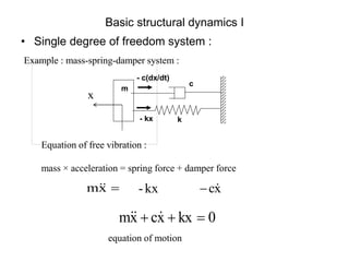
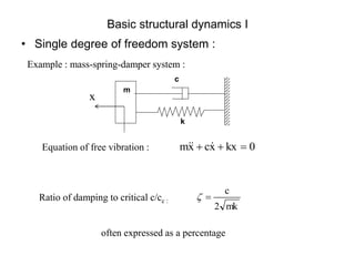
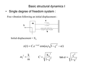
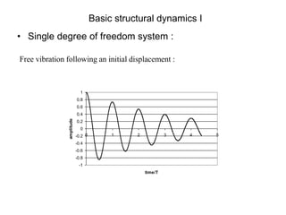
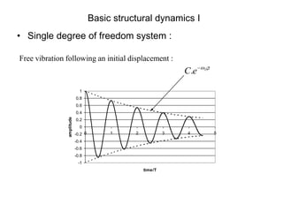
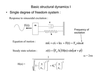
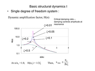
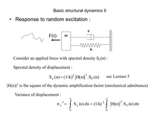
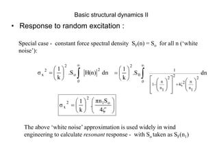
This document is a lecture on basic structural dynamics with a focus on wind loading and structural response. It covers topics such as single degree-of-freedom systems, equations of free vibration, response to sinusoidal and random excitation, and dynamic amplification factors. The content is aimed at providing foundational knowledge in structural dynamics relevant to engineering applications.

1. Basic structural dynamics I
Wind loading and structural response - Lecture 10
Dr. J.D. Holmes

2. Basic structural dynamics I
• Topics :
• Revision of single degree-of freedom vibration theory
• Response to sinusoidal excitation
Refs. : R.W. Clough and J. Penzien ‘Dynamics of Structures’ 1975
R.R. Craig ‘Structural Dynamics’ 1981
J.D. Holmes ‘Wind Loading of Structures’ 2001
• Multi-degree of freedom structures – Lect. 11
• Response to random excitation

3. Basic structural dynamics I
x
c

Equation of free vibration :
Example : mass-spring-damper system :
k
c
m
x
0
kx
x
c
x
m 

 


mass × acceleration = spring force + damper force
- kx
- c(dx/dt)

x
m 
 kx
-
equation of motion
• Single degree of freedom system :

4. Basic structural dynamics I
• Single degree of freedom system :
Equation of free vibration :
Example : mass-spring-damper system :
Ratio of damping to critical c/cc :
k
c
m
x
0
kx
x
c
x
m 

 


mk
2
c


often expressed as a percentage

5. Basic structural dynamics I
• Single degree of freedom system :
Damper removed :
k
m
x(t)
Equation of motion : 0
kx
x
m 



x
m
kx 



is an equivalent static force (‘inertial’ force)
x
m


Undamped natural frequency :


2
m
k
2π
1
n 1
1 

Period of vibration, T :
1
1
1
2
T
n





6. Basic structural dynamics I
• Single degree of freedom system :
Initial displacement = Xo
Free vibration following an initial displacement :
k
c
m
x
m
k
2
1 

)
1
cos(
.
)
( 2
1
1







 
t
e
C
t
x t
2
2
0
-
1
X


C 2
2
-
1
tan


 

7. Basic structural dynamics I
• Single degree of freedom system :
Free vibration following an initial displacement :
-1
-0.8
-0.6
-0.4
-0.2
0
0.2
0.4
0.6
0.8
1
0 1 2 3 4 5
time/T
amplitude

8. Basic structural dynamics I
• Single degree of freedom system :
Free vibration following an initial displacement :
-1
-0.8
-0.6
-0.4
-0.2
0
0.2
0.4
0.6
0.8
1
0 1 2 3 4 5
time/T
amplitude t
e
C 
1
. 

9. Basic structural dynamics I
• Single degree of freedom system :
Response to sinusoidal excitation :
Equation of motion :
t
sin
F
F(t)
kx
x
c
x
m o 



 


Steady state solution :    

 
 t
x sin
H(n)
/k
F
(t) o
k
c
m
F(t)
 = 2n
H(n) =
2
1
2
2
2
1 n
n
4ζ
n
n
1
1


























Frequency of
excitation

10. Basic structural dynamics I
• Single degree of freedom system :
Critical damping ratio –
damping controls amplitude at
resonance
0.1
1.0
10.0
100.0
0 1 2 3 4
n/n1
H(n)
=0.01
=0.05
=0.1
=0.2
=0.5
At n/n1 =1.0, H(n1) = 1/2 Then, 2kζ
F
x 0
max 
Dynamic amplification factor, H(n)

11. Basic structural dynamics II
• Response to random excitation :
Consider an applied force with spectral density SF(n) :
dn
(n)
.S
H(n)
.
(1/k)
dn
(n)
S
σ F
2
0
2
x
0
2
x 





k
c
m
F(t)
Spectral density of displacement :
|H(n)|2 is the square of the dynamic amplification factor (mechanical admittance)
(n)
.S
H(n)
.
(1/k)
(n)
S F
2
2
x 
Variance of displacement :
see Lecture 5

12. Basic structural dynamics II
• Response to random excitation :
Special case - constant force spectral density SF(n) = So for all n (‘white
noise’):
dn
H(n)
.S
k
1
σ
2
o
2
2
x 








0
The above ‘white noise’ approximation is used widely in wind
engineering to calculate resonant response - with So taken as SF(n1)
dn
.S
k
1
2
1
n
n
2
4ζ
2
2
1
n
n
1
1
0
2































0
















4
S
πn
.
k
1
σ o
1
2
2
x

13. End of Lecture
John Holmes
225-405-3789 JHolmes@lsu.edu