This document is the copyright page and contents for the World Bank's 2016 report "Poverty and Shared Prosperity". It acknowledges the staff and external contributors to the report. It also outlines the open license terms for reuse and distribution of the report's content. The report aims to provide the latest statistics and analysis on global poverty reduction and increasing shared prosperity.


![2
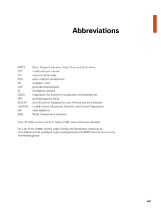
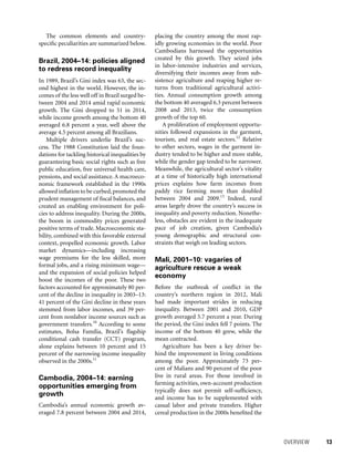
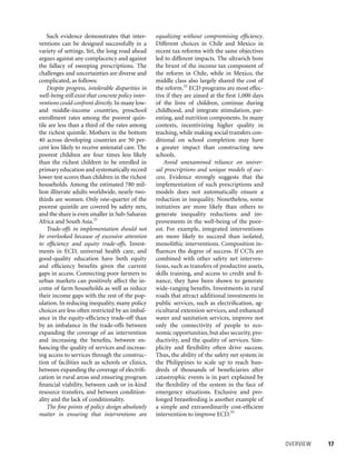
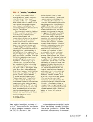
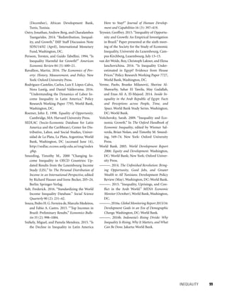
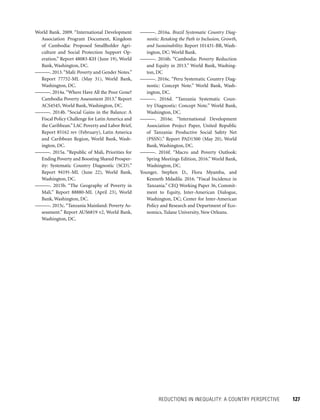
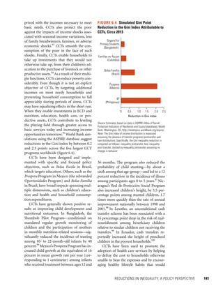
Chapter 2 presents the latest data on global and regional poverty using the international
extreme poverty line of US$1.90 (2011 purchasing power parity [PPP] U.S. dollars). The
chapter discusses the geographical concentration of poverty and complements the global
headcount ratio and data by providing a profile of global poverty. It also reflects on recent
methodological changes and their consequences on global estimates.
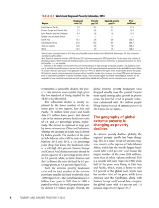
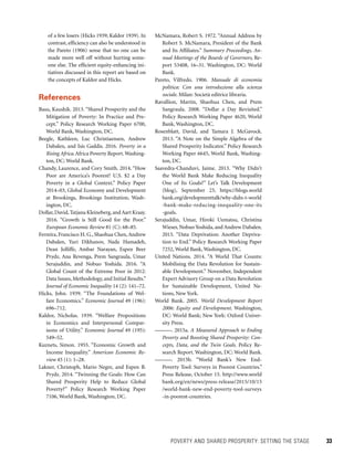
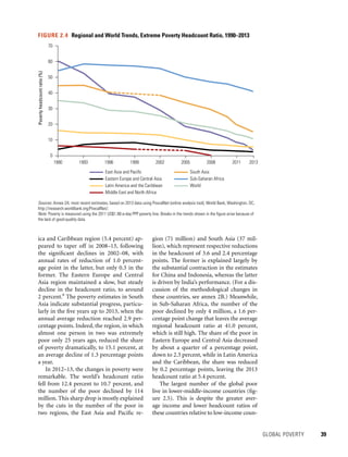
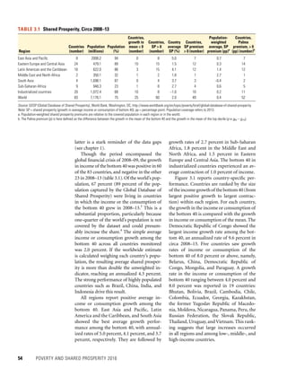
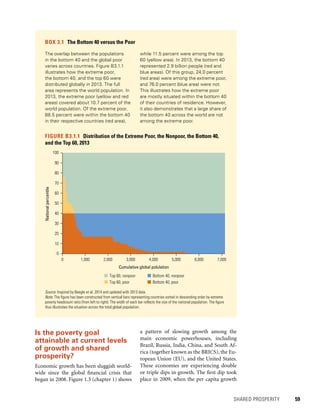
The global poverty estimate for 2013 is 10.7 percent of the world’s population, or 767
million people. This confirms the continuation of the rapid downward trend in the poverty
headcount ratio since 1990 (an average of 1.1 percentage points per year). The reduc-
tion in 2013 is even greater than the average, with a decline in the headcount ratio of 1.7
percentage points. In absolute net terms, this represents 114 million fewer poor people in
a single year. Much of the observed reduction was driven by remarkable progress in the
East Asia and Pacific region (71 million fewer poor) and South Asia (37 million fewer poor).
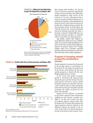
A significant change in the geography of poverty has meant that Sub-Saharan Africa was
hosting more than half the world’s poor in 2013. This is despite the fact that the African
subcontinent experienced progress in lowering both the headcount ratio (1.6 percentage
points) and the number of the poor (4 million in 2012–13). However, these achievements are
modest compared with reductions in East Asia and Pacific and in South Asia. Other regions
with lower poverty rates and totals—notably, Eastern Europe and Central Asia, as well as
Latin America and the Caribbean—saw marginal declines in 2012–13. The profile of the
global poor shows they are predominantly rural, young, poorly educated, mostly employed in
the agricultural sector, and living in larger households with more children.
Global Poverty
GLOBAL POVERTY 35
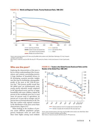
Ever since the first World Development
Report, World Development Report 1990:
Poverty, the share of people living on less
than US$1.90 per person per day has been
steadily declining.1
This has occurred at a
rapid average pace of 1.1 percentage points
a year. Overall, the total number of poor
has also decreased steadily and dramati-
cally throughout the period, except for the
1997–99 span of increasing poverty associ-
ated with the Asian financial crisis. Signifi-
cant progress in poverty reduction has been
accompanied by important improvements
in data availability, although substantial
gaps remain (see chapter 1). As a result,
the global poverty headcount in 2013 in-
corporated survey-based estimates on 137
countries.2
In 2013, an estimated 767 million peo-
ple were living under the international pov-
erty line of US$1.90 a day (table 2.1). This
means that almost 11 people in 100, or 10.7
Monitoring global poverty](https://image.slidesharecdn.com/banquemondialepauvret-161004082852/85/Banque-mondiale-pauvrete-55-320.jpg)
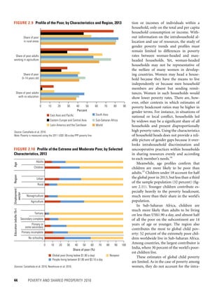


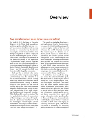
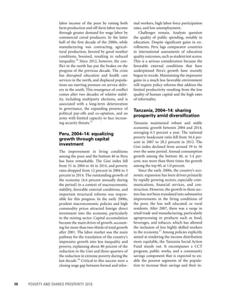
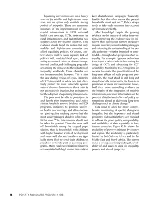
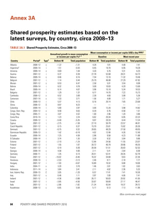
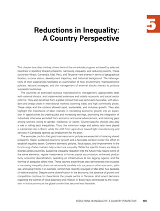
![SHARED PROSPERITY 57
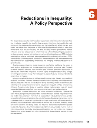
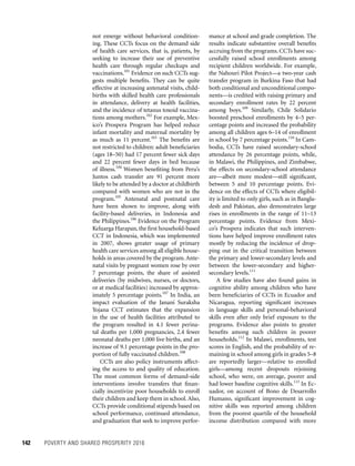
ically larger in absolute terms than the gain
of the average household in the bottom 40.
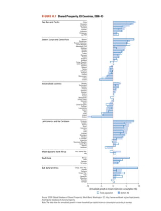
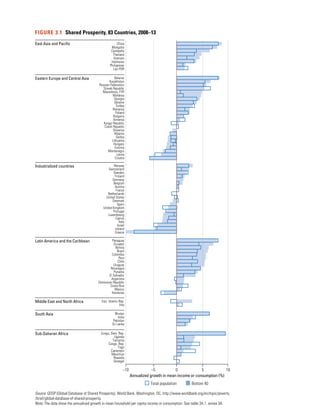
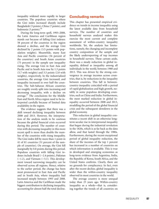
Of the 83 countries in the sample in
2008–13, the income or consumption of
the bottom 40 in 52 countries grew more
quickly relative to the top 10, while the op-
posite occurred in the remaining 31 coun-
tries. The differences in the growth rates of
the bottom 40 and the top 10 are reported
in the Palma premium column in table 3.1.
The larger number of countries with pos-
itive Palma premiums suggests that more
countries experienced narrowing income
inequality than widening inequality over
the period. An examination of the Gini
index in a separate dataset—PovcalNet—
confirms this (see chapter 4).8
These en-
couraging results were driven primarily
by three regions, namely, East Asia and
Pacific, Latin America and the Caribbean,
and South Asia.
Care should be taken in interpreting
these results, however, given the well-known
shortcomings in household survey data,
from which the Palma premium is calcu-
lated, namely, the high rates of survey non-
response at the top; the underreporting of
incomes, particularly (but not only) capital
incomes; and the use of consumption (in-
stead of incomes) in many countries, thus
omitting the greater savings at the top.9
Who are the bottom 40?
People in the bottom 40 differ in income
or consumption across countries. They
also differ in other dimensions of well-
being such as the educational performance
of children, women’s access to health care
services, food insecurity and child stunting,
access to safe water, and access to the Inter-
net, as recently detailed in the World Bank
Global Monitoring Report 2015/16.10
Moreover, the populations monitored
to construct the indicator of the growth in
income or consumption among the bot-
tom 40 differ from the global extreme poor.
Measured according to the global poverty
line of US$1.90 (2011 purchasing power
parity [PPP]) per person a day, all the poor
in, say, Brazil, China, Honduras, India, or
South Africa have similar incomes below
the monetary threshold, that is, less than
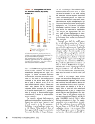
but this only includes a limited sample of 2
countries.
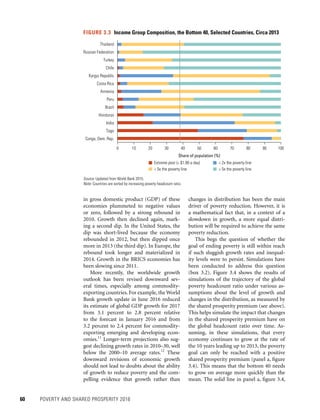
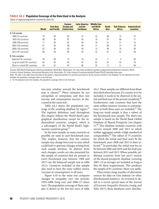
The average population-weighted shared
prosperity premium is positive in all re-
gions, save South Asia, where India’s large
population and negative premium heavily
influences the negative regional average.
In the remaining regions, the shared pros-
perity premiums are positive: under 1 per-
centage point in East Asia and Pacific (0.7),
Eastern Europe and Central Asia (0.3), and
Sub-Saharan Africa (0.6) and in excess of 1
percentage point in Latin America and the
Caribbean (1.4) and the Middle East and
North Africa (2.7). Industrialized countries
have a meager shared prosperity premium
of only 0.2 percentage points.
The share of countries that experienced
a positive shared prosperity premium was
practically the same in circa 2008–13 as in
2007–12. Around 60 percent of the coun-
tries in the sample reported a positive pre-
mium in both rounds. This comparison re-
quires caution, however. Possible changes in
the shares of countries with positive premi-
ums respond to changes both in the growth
performance of countries and in the com-
position of the sample of countries, and the
impact of the latter can easily dominate that
of the former.
Incomes of the bottom 40
and the top 10: the Palma
premium
The shared prosperity premium fails to
capture much of the variation in incomes
that affects the topmost earners. To account
for such intragroup differences, especially
among the top earners, an indicator com-
paring income growth among the bottom
40 and the top 10 is used, the Palma pre-
mium.7
Similar to the shared prosperity pre-
mium, which compares the relative growth
in income or consumption among the bot-
tom 40 and the mean, the Palma premium
reports the growth rate in income or con-
sumption among the bottom 40, minus the
growth rate in the top 10. Even if the top 10
achieves lower income growth than the bot-
tom 40, the income or consumption gain of
the average household in the top 10 is typ-](https://image.slidesharecdn.com/banquemondialepauvret-161004082852/85/Banque-mondiale-pauvrete-77-320.jpg)


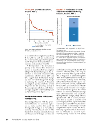
![104 POVERTY AND SHARED PROSPERITY 2016
individual incomes of top earners, confirms
the decline in the Gini, but at a more mod-
est pace.3
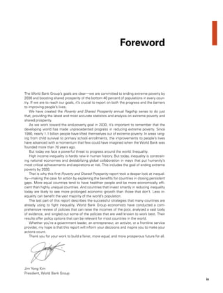
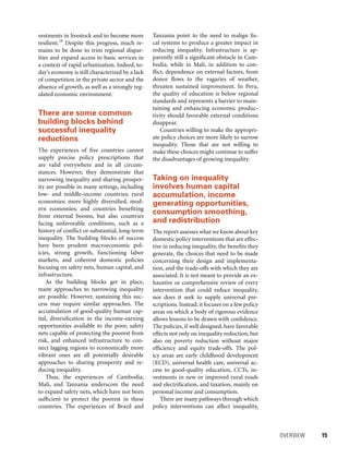
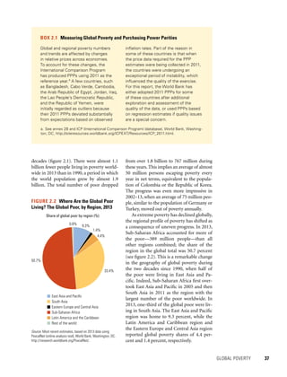
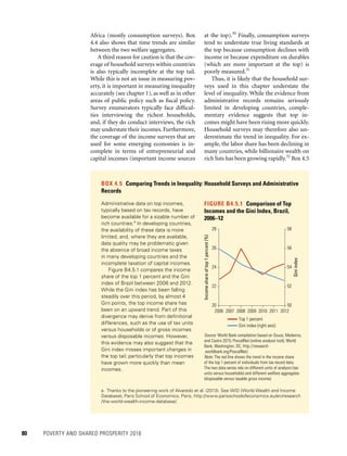
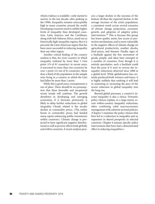
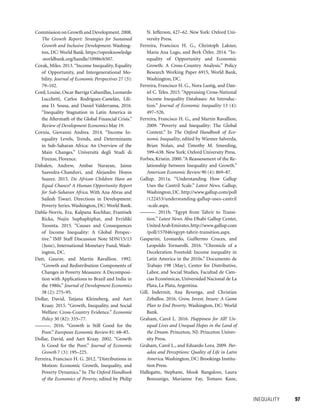
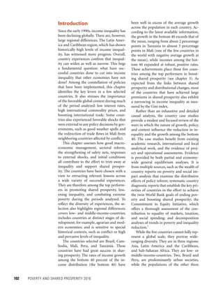
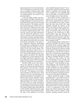
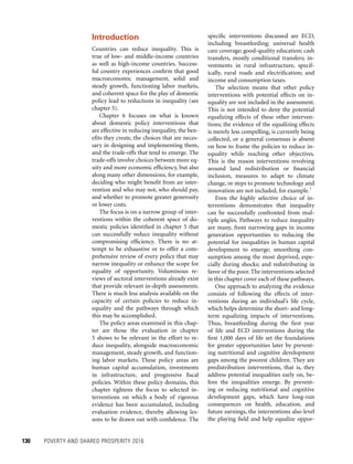
The marked drop in income inequal-
ity helped translate economic growth into
large poverty reductions. Between 2004 and
2014, 26.5 million Brazilians exited pov-
erty.4
While 22 in every 100 people were
living on an income of less than R$140 a
month in 2004, this was only true of 7 in
100 Brazilians 10 years later.5
The share of
the population living on less than US$1.90
a day (in 2011 purchasing power parity
[PPP] U.S. dollars) fell from 11.0 percent
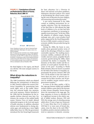
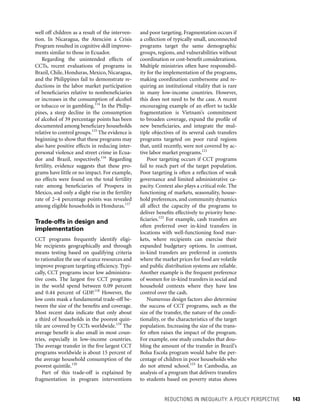
to 3.7 percent during the period. Decom-
position exercises conclude that about 60
percent of this reduction was caused by the
average increase in incomes among Brazil-
ian households (the growth effect), while
the remaining 40 percent can be attributed
to improvements in income distribution
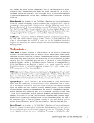
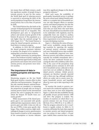
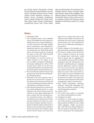
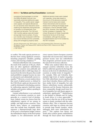
among Brazilians (figure 5.3).
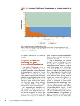
Despite these achievements, the country
is still highly unequal. In 2014, the bottom
40 held approximately 12 percent of total
income, while the top 20 held 56 percent.6
That year, Brazil’s Gini index of 51, while
notably lower than 10 years previously, was
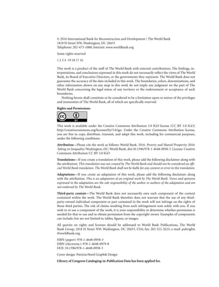
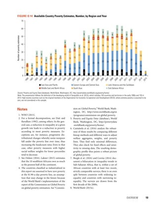
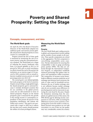
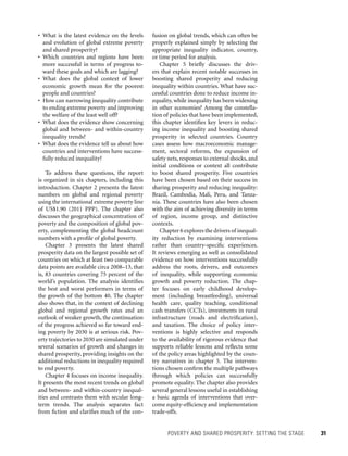
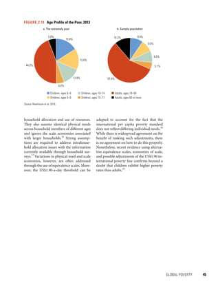
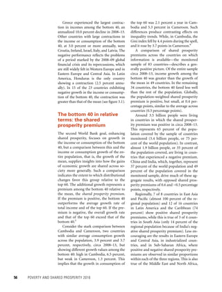
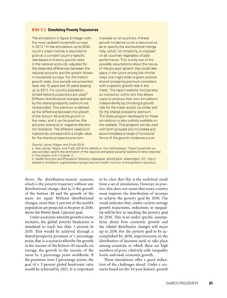
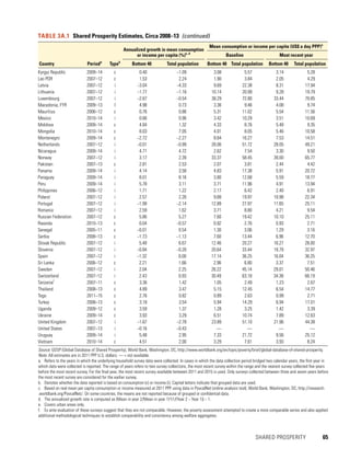
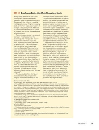
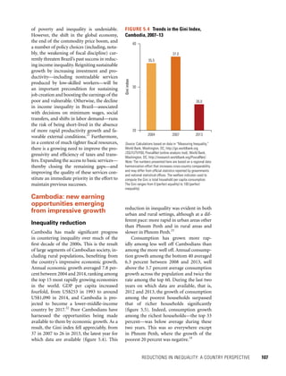
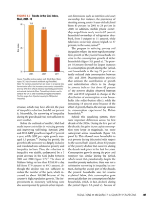
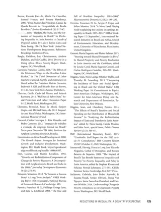
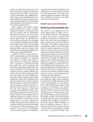
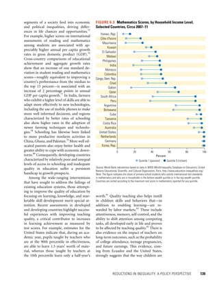
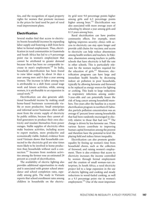
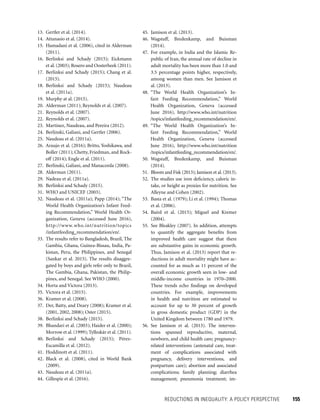
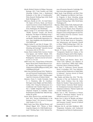
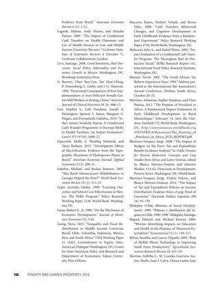
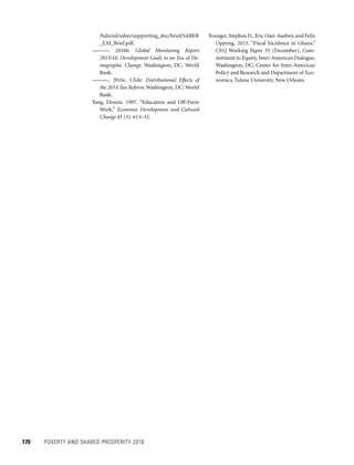
The incomes of the less well off surged
between 2004 and 2014 amid rapid eco-
nomic growth. Figure 5.2 shows that the
average annual growth in the incomes of
the bottom 10 doubles that of the top 10.
The World Bank’s indicator of shared pros-
perity—the growth rate of household in-
come per capita of the bottom 40—high-
lights how Brazil’s growth in the recent past
has disproportionally benefited the poorest
households. Between 2004 and 2014, the
income growth among the bottom 40 aver-
aged 6.8 percent a year, compared with 4.5
percent for the average Brazilian. Over the
same period, incomes among the bottom
40 in Brazil rose at the second fastest rate in
the region, only surpassed by Bolivia. This
suggests that most of the decline in overall
inequality occurred because of a reduction
in inequality at the bottom of the income
distribution. Alternative evidence drawing
on tax records, which are more effective
than household surveys at capturing the
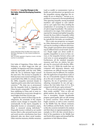
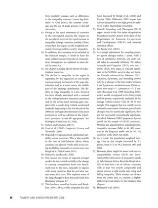
FIGURE 5.1 Trends in the Gini Index, Brazil, 1981–2014
Sources: Tabulations of Equity Lab, Team for Statistical Development, World Bank, Washington, DC, based
on data in the SEDLAC database; WDI (World Development Indicators) (database), World Bank, Washing-
ton, DC, http://data.worldbank.org/data-catalog/world-development-indicators; PovcalNet (online analysis
tool), World Bank, Washington, DC, http://iresearch.worldbank.org/PovcalNet/.
Note: The data are based on a regional data harmonization effort that increases cross-country com
parability and may differ from official statistics reported by governments and national statistical offices.
The welfare indicator used to compute the Gini is household per capita income. The Gini ranges from
0 (perfect equality) to 100 (perfect inequality). The Latin America and Caribbean aggregate is based on
17 countries in the region on which microdata are available. The Gini index of the Latin America and
Caribbean region is computed based on pooled country-specific data previously collapsed into 8,000
percentiles. In cases where data are unavailable for a given country in a given year, values have been
interpolated by projecting incomes for that year based on GDP growth and assuming no changes in the
distribution of incomes in the interpolated year. Dotted lines cover years in which data are not available
or present quality issues.
Giniindex
50
52
54
56
58
60
62
64
1981 198419871990 1993 19961999 20022005 2008 2011 2014
Brazil Latin America and the Caribbean
FIGURE 5.2 Growth Incidence Curve,
Brazil, 2004–14
Source: Tabulations of Equity Lab, Team for Statistical Devel-
opment, World Bank, Washington, DC, based on data in the
SEDLAC database.
Annualgrowthrate(%)
0
1
2
3
4
5
6
7
8
5 20 35 50 65 80 95
Income percentile
Annualized growth of percentile
Average growth](https://image.slidesharecdn.com/banquemondialepauvret-161004082852/85/Banque-mondiale-pauvrete-124-320.jpg)


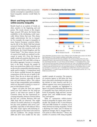
![REDUCTIONS IN INEQUALITY: A POLICY PERSPECTIVE 159
a reduction of over 7 points in the market
income Gini, is an exception among mod-
erate redistributive effects. Redistribution
is associated with a reduction in the market
income Gini of about 1–3 points in Ethio-
pia, Jordan, and Sri Lanka; the reductions
are larger in Georgia and Russia. See In-
chauste and Lustig (forthcoming); Lustig
(2015); Younger, Osei-Assibey, and Op-
pong (2015).
174. See IMF (2014). For example, personal
income taxation in developing countries
raises an average 1–3 percent of GDP, com-
pared with 9–11 percent of GDP among
advanced countries.
175. Country-by-country comparative results
need to viewed with caution, however. They
are derived based on different methodolo-
gies (incidence analysis versus ex ante simu-
lations), the indicator analyzed (income or
consumption), conventions (the treatment
of pension income), and the categories in-
cluded (health care and education spend-
ing). This implies that the analyses cover
different (but always incomplete) segments
of the fiscal system. See Inchauste and
Lustig (forthcoming).
References
Abramovsky, Laura, Orazio Attanasio, Kai
Barron, Pedro Carneiro, and George Stoye.
2014. “Challenges to Promoting Social In-
clusion of the Extreme Poor: Evidence from
a Large Scale Experiment in Colombia.” IFS
Working Paper W14/33, Institute for Fiscal
Studies, London.
Aggarwal, Shilpa. 2015. “Do Rural Roads Create
Pathways out of Poverty? Evidence from
India.”Working paper, Indian School of Busi-
ness, Hyderabad, India.
Ahmed, Shakil, and Chris Morgan. 2011.
“Demand-Side Financing for Maternal
Health Care: The Current State of Knowledge
on Design and Impact.” Issues Brief 1 (Sep-
tember), Nossal Institute for Global Health,
University of Melbourne, Melbourne.
Aker, Jenny, Rachid Boumnijel, Amanda
McClelland, and Niall Tierney. 2013. “How
Do Electronic Transfers Compare? Evidence
from a Mobile Money Cash Transfer Experi-
ment in Niger.” Technical Report, Tufts Uni-
versity, Medford, MA.
161. Some countries, such as Colombia, Na-
mibia, the Russian Federation, South Af-
rica, and Uruguay, collect more than 1
percent of GDP as recurrent property taxes
(Broadway, Chamberlain, and Emmerson
2010; de Ferranti et al. 2004; IMF 2014;
Martinez-Vasquez 2008; World Bank 2005).
162. Lustig (2015).
163. Direct taxes cause the more well off to bear
the brunt, while indirect taxes cause the
poor to bear a larger relative share of the
burden, given that the poor spend a higher
share of their incomes on consumption.
164. Bird and Zolt (2003).
165. Sahn and Younger (2000).
166. Yet, large country variations are observed
across the EU. Reductions in market in-
equalities are large in Western Europe,
but much more limited in the Baltic States
(Avram, Levy, and Sutherland 2014; De
Agostini, Palaus, and Tasseva 2015).
167. See Martinez-Vasquez, Vulovic, and
Moreno-Dodson (2014). Taxes are respon-
sible for an average increase of 1.5 percent
in the Gini index of market incomes in the
country sample since 1990.
168. Bird and Zolt (2003, 2008).
169. According to the definition of Ravallion
(2009), poor countries show consumption
per capita under US$2,000 a year (2005
purchasing power parity [PPP] U.S. dol-
lars).However,the more well off developing
countries—countries with consumption
per capita at US$4,000 per year—would re-
quire little additional taxation on the rich
to eliminate extreme poverty. (Additional
marginal tax rates between 1 percent and 6
percent would be required.) In each coun-
try, a rich household is a household that,
in the United States, would be categorized
as nonpoor. No economic distortions, be-
havioral changes, or political economy or
administrative considerations are taken
into account in the analysis, which includes
90 countries on which there are data for
around the late 2000s.
170. Hoy and Sumner (2016).
171. Ostry, Berg, and Tsangarides (2014).
172. Inchauste and Lustig (forthcoming); Lustig
(2015).
173. Redistributive effects range from less than
1 point to over 4 points (in Brazil) of the
Gini for market incomes. South Africa with](https://image.slidesharecdn.com/banquemondialepauvret-161004082852/85/Banque-mondiale-pauvrete-179-320.jpg)


![Fullreport[1]](https://cdn.slidesharecdn.com/ss_thumbnails/fullreport1-120214140553-phpapp01-thumbnail.jpg?width=640&height=640&fit=bounds)


