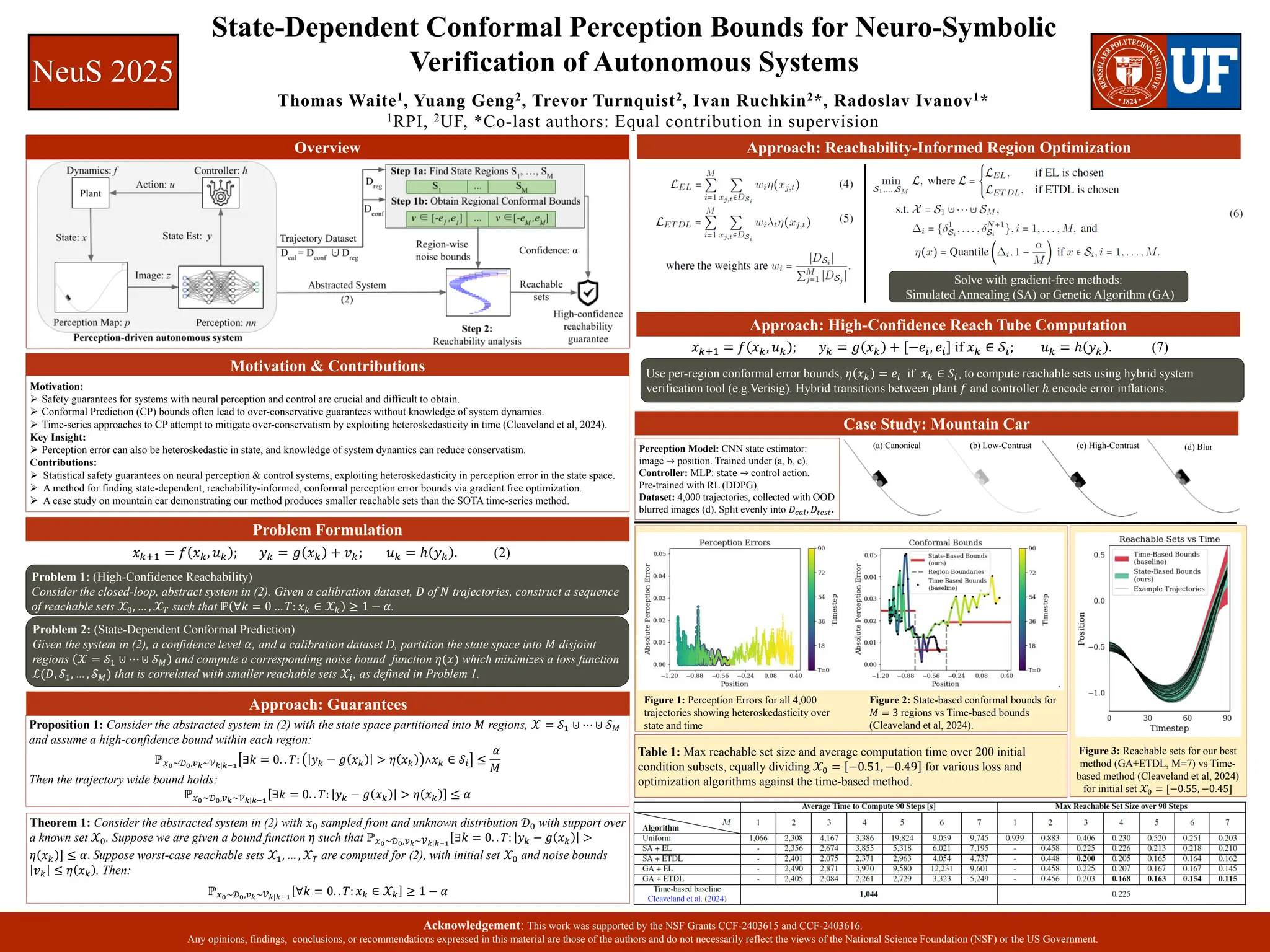
A poster presented by Thomas Waite and Radoslav Ivanov at the 2nd International Conference on Neuro-symbolic Systems (NeuS) in May 2025. Paper: https://arxiv.org/abs/2502.21308 Abstract: It remains a challenge to provide safety guarantees for autonomous systems with neural perception and control. A typical approach obtains symbolic bounds on perception error (e.g., using conformal prediction) and performs verification under these bounds. However, these bounds can lead to drastic conservatism in the resulting end-to-end safety guarantee. This paper proposes an approach to synthesize symbolic perception error bounds that serve as an optimal interface between perception performance and control verification. The key idea is to consider our error bounds to be heteroskedastic with respect to the system's state -- not time like in previous approaches. These bounds can be obtained with two gradient-free optimization algorithms. We demonstrate that our bounds lead to tighter safety guarantees than the state-of-the-art in a case study on a mountain car.

1. State-Dependent Conformal Perception Bounds for Neuro-Symbolic
Verification of Autonomous Systems
Motivation & Contributions
Motivation:
➢ Safety guarantees for systems with neural perception and control are crucial and difficult to obtain.
➢ Conformal Prediction (CP) bounds often lead to over-conservative guarantees without knowledge of system dynamics.
➢ Time-series approaches to CP attempt to mitigate over-conservatism by exploiting heteroskedasticity in time (Cleaveland et al, 2024).
Key Insight:
➢ Perception error can also be heteroskedastic in state, and knowledge of system dynamics can reduce conservatism.
Contributions:
➢ Statistical safety guarantees on neural perception & control systems, exploiting heteroskedasticity in perception error in the state space.
➢ A method for finding state-dependent, reachability-informed, conformal perception error bounds via gradient free optimization.
➢ A case study on mountain car demonstrating our method produces smaller reachable sets than the SOTA time-series method.
Problem 1: (High-Confidence Reachability)
Consider the closed-loop, abstract system in (2). Given a calibration dataset, 𝐷 of 𝑁 trajectories, construct a sequence
of reachable sets 𝒳0, … , 𝒳𝑇 such that ℙ ∀𝑘 = 0 … 𝑇: 𝑥𝑘 ∈ 𝒳𝑘 ≥ 1 − 𝛼.
Problem 2: (State-Dependent Conformal Prediction)
Given the system in (2), a confidence level 𝛼, and a calibration dataset D, partition the state space into 𝑀 disjoint
regions 𝒳 = 𝒮1 ⊍ ⋯ ⊍ 𝒮𝑀 and compute a corresponding noise bound function 𝜂(𝑥) which minimizes a loss function
ℒ(𝐷, 𝒮1, … , 𝒮𝑀) that is correlated with smaller reachable sets 𝒳𝑖, as defined in Problem 1.
Acknowledgement: This work was supported by the NSF Grants CCF-2403615 and CCF-2403616.
Any opinions, findings, conclusions, or recommendations expressed in this material are those of the authors and do not necessarily reflect the views of the National Science Foundation (NSF) or the US Government.
𝑥𝑘+1 = 𝑓 𝑥𝑘, 𝑢𝑘 ; 𝑦𝑘 = 𝑔 𝑥𝑘 + 𝑣𝑘; 𝑢𝑘 = ℎ 𝑦𝑘 . (2)
Problem Formulation
Thomas Waite1, Yuang Geng2, Trevor Turnquist2, Ivan Ruchkin2*, Radoslav Ivanov1*
1RPI, 2UF, *Co-last authors: Equal contribution in supervision
Solve with gradient-free methods:
Simulated Annealing (SA) or Genetic Algorithm (GA)
Use per-region conformal error bounds, 𝜂 𝑥𝑘 = 𝑒𝑖 if 𝑥𝑘 ∈ 𝑆𝑖, to compute reachable sets using hybrid system
verification tool (e.g.Verisig). Hybrid transitions between plant 𝑓 and controller ℎ encode error inflations.
Perception Model: CNN state estimator:
image → position. Trained under (a, b, c).
Controller: MLP: state → control action.
Pre-trained with RL (DDPG).
Dataset: 4,000 trajectories, collected with OOD
blurred images (d). Split evenly into 𝐷𝑐𝑎𝑙, 𝐷𝑡𝑒𝑠𝑡.
(a) Canonical (b) Low-Contrast (c) High-Contrast (d) Blur
Overview
Approach: Guarantees
Proposition 1: Consider the abstracted system in (2) with the state space partitioned into 𝑀 regions, 𝒳 = 𝒮1 ⊍ ⋯ ⊍ 𝒮𝑀
and assume a high-confidence bound within each region:
ℙ𝑥0~𝒟0,𝑣𝑘~𝒱𝑘|𝑘−1
∃𝑘 = 0. . 𝑇: 𝑦𝑘 − 𝑔 𝑥𝑘 > 𝜂 𝑥𝑘 ˄𝑥𝑘 ∈ 𝒮𝑖 ≤
𝛼
𝑀
Then the trajectory wide bound holds:
ℙ𝑥0~𝒟0,𝑣𝑘~𝒱𝑘|𝑘−1
∃𝑘 = 0. . 𝑇: 𝑦𝑘 − 𝑔 𝑥𝑘 > 𝜂 𝑥𝑘 ≤ 𝛼
Theorem 1: Consider the abstracted system in (2) with 𝑥0 sampled from and unknown distribution 𝒟0 with support over
a known set 𝒳0. Suppose we are given a bound function 𝜂 such that ℙ𝑥0~𝒟0,𝑣𝑘~𝒱𝑘|𝑘−1
ሾ
ሿ
∃𝑘 = 0. . 𝑇: 𝑦𝑘 − 𝑔 𝑥𝑘 >
𝜂 𝑥𝑘 ≤ 𝛼. Suppose worst-case reachable sets 𝒳1, … , 𝒳𝑇 are computed for (2), with initial set 𝒳0 and noise bounds
𝑣𝑘 ≤ 𝜂 𝑥𝑘 . Then:
ℙ𝑥0~𝒟0,𝑣𝑘~𝒱𝑘|𝑘−1
∀𝑘 = 0. . 𝑇: 𝑥𝑘 ∈ 𝒳𝑘 ≥ 1 − 𝛼
Approach: Reachability-Informed Region Optimization
Approach: High-Confidence Reach Tube Computation
𝑥𝑘+1 = 𝑓 𝑥𝑘, 𝑢𝑘 ; 𝑦𝑘 = 𝑔 𝑥𝑘 + −𝑒𝑖, 𝑒𝑖 if 𝑥𝑘 ∈ 𝒮𝑖; 𝑢𝑘 = ℎ 𝑦𝑘 . (7)
Case Study: Mountain Car
Figure 1: Perception Errors for all 4,000
trajectories showing heteroskedasticity over
state and time
Figure 2: State-based conformal bounds for
𝑀 = 3 regions vs Time-based bounds
(Cleaveland et al, 2024).
Figure 3: Reachable sets for our best
method (GA+ETDL, M=7) vs Time-
based method (Cleaveland et al, 2024)
for initial set 𝒳0 = ሾ−0.55, −0.45ሿ
Table 1: Max reachable set size and average computation time over 200 initial
condition subsets, equally dividing 𝒳0 = −0.51, −0.49 for various loss and
optimization algorithms against the time-based method.
NeuS 2025