This document provides a methodology for evaluating the seismic performance of existing concrete buildings and developing retrofit strategies. It was developed by the Applied Technology Council through funding from the California Seismic Safety Commission as part of the Proposition 122 Seismic Retrofit Practices Improvement Program. The methodology is presented in two volumes and includes guidelines for determining a building's deficiencies, developing and selecting from alternative retrofit strategies, performing nonlinear analysis, establishing modeling rules, evaluating foundation effects, setting response limits, and addressing nonstructural components. The methodology aims to provide concise summaries to assess seismic performance and develop cost-effective retrofit solutions to meet performance objectives.

1. ATe
E!1
Seismic evaluation and retrofit
of concrete buildings
Volume 1
aTe
...... 0
•
Applied Technology Council
TN
._~ .~ CALIFORNIA SEISMIC SAFETY COMMISSION
o
,
. t'L 4 . J..:U":l:.
~
A'Ic,S
.
Proposition 122 Seismic Retrofit Practices Improvement Program
Report
.,
",
sse 96-01
...

2. (
(

3. ATC-4D
i,..<--
Seismic Evaluation and Retrofit
of
Concrete Buildings
Volume 1
by
APPLIED TECHNOLOGY COUNCIL
555. Twin Dolphin Drive, Suite 550
Redwood City, California 94065
Funded by
SEISMIC SAFETY COMMISSION
State of California
Products 1.2 and 1.3 of the Proposition 122
Seismic Retrofit Practices Improvement Program
PRlNCIPAL :INVESTIGATOR
Craig D. Comartin
CO-PRINCIPAL IN''"VESTIGATOR
PRQJECT DIRECTOR
Richard W. Niewiarowski
SENIOR ADVISOR
Christopher Rojabn
II " 11I1 If 1111
2494/R
Report No. sse 96-01
November 1996
''l
..... ~
.,-~~

4. (
I
:
(
(
(
(
(
(
;-
1:

5. Preface
Proposition 122 passed by California's voters in
1990, created the Earthquake Safety and Public
Buildings Rehabilitation Fund of 1990, supported by a $300 million general obligation
bond program for the seismic retrofit of state
_
and local government buildings. As a part of
the program, Proposition 122 authorizes the
California Seismic Safety Commission (CSSC).
to use up to 1% of the proceeds of the bonds, or
approximately $3 million, to carry out a range
of activities that will capitalize on the seismic
retrofit experience in the private sector to improve seismic retrofit practices for government
buildings. The purpose of California's Proposition 122 research and development program is
to develop state-of-the-practice recommendations to address current needs for seismic retrofit provisions and seismic risk decision tools. It
is focused specifically on vulnerable concrete
structures consistent with the types of concrete
buildings that make up a significant portion of
California's state and local government inventories.
In 1994, as part of the Proposition 122 Seismic
Retrofit Practices Improvement Program, the
Commission awarded the Applied Technology
Council (ATC) a contract to develop a recommended methodology and commentary for the
seismic evaluation and retrofit of existing concrete buildings (product 1.2). In 1995·the
Commission awarded a second, related contract
to ATC to expand the Product 1.2 effort to include effects of foundations on the seismic performance of existing concrete buildings
(Product 1.3). The results of the two projects
have been combined and are presented in this
ATC-40 Report (also known as SSC-96-01).
TV/o other reports recently published by the
California Seismic Safety Commission, the
Provisional Commentary for Seismic Retrofit
(1994) and the Review of Seismic Research Results on Existing Buildings (1994), are Products
1.1 and 3.1 of the Proposition 122 Program, respectively. These two previous reports provide
the primary basis for the development of the
recommended methodology and commentary
contained in this document.
. This document is organized into two volumes.
Volume One contains the main body of the
evaluation and retrofit methodology, presented
in 13 chapters, with a glossary and a list of ref_erences, J1d~ volume contains all ofthe parts of
the document required for the' evaluation and
retrofit of btrildings. Volume Two consists of
Appendices containing supporting materials related to the methodology: four example building
case study reports, a cost effectiveness study
related to the four building studies, and a review
of research on the effects of foundation conditions on the seismic performance of concrete
buildings.
This report was prepared under the direction of
ATe Senior Consultant Craig Comartin, who
served as Principal Investigator, and Richard W.
Niewiarowski, who served as Co-Principal Investigator and Project Director. Fred Turner
served as esse Project Manager. Overview
and guidance were provided by the Proposition
122 Oversight Panel consisting of Frederick M.
Herman (Chair), Richard Conrad, Ross Cranmer, Wilfred Iwan, Roy Johnston, Frank
McClure, Gary McGavin, Joel McRonald, J 0seph P. Nicoletti, Stanley Scott, and Lowell
Shields. The Product 1.2 methodology and
commentary were prepared by Sigmund A.
Freeman, Ronald o. Hamburger, William T.
Holmes, Charles Kircher, Jack P: Moehle,
Thomas A. Sabol, and N abib. Youssef (Product
1.2 Senior Advisory Panel). The Product 1.3
GeotechnicallStructural Working Group consisted of Sunil Gupta, Geoffrey Martin, Marshall Lew, and Lelio Mejia. William T.Holmes, Yoshi Moriwaki, Maurice Power and
Nabih Youssef served on the Product ~.3 Senior
Advisory Panel. Gregory P. Luth and Tom H.
Hale, respectively, served as the Quality .A,..SSUfance Consultant and the Cost Effectiveness
Study Consultant. Wendy Rule served as Technical Editor, and Gail Hynes Shea served as
Publications Consultant.
Richard McCarthy
CSSC Executive Director
Christopher Rojahn
ATC Executive Director & ATC-40" Senior
Advisor

6. :
.·oversight. Panei far·
._----- ~Propositla~-,-2-2--5eism·ic .Re~roFrt· -pracflces-------- --._-.--' . .
.
Improvement program
Frederick M. Herman, Chair
Seismic Safety Commission
Local Government/Building
Official
Stanley Scott
Research Political Scientist
Frank McClure
Structural Engineer
Joel McRonald
Division of the State Architect
Gary McGavin
Seismic Safety Commission
Architect
Ross Cranmer
Building Official
Roy Johnston
Structural Engineer
Dr. Wilfred Iwan
Mechanical Engineer
Richard Conrad
Building Standards Commission
Joseph P. Nicoletti
Structural Engineer
Structural Engineer
Lowell E: Shields
Seismic Safety Commission
Mechanical Engineer
(
(
(
~
-e :
(
(
;.
S~ismi~
Safety
Commission Staff
Richard McCarthy
Executive Director
Fred Turner
Project Manager
Karen Cogan
Deborah Penny
Carmen Marquez
Chris Lindstrom
Ed Hensley
Ten DeVriend
Kathy Goodell
(
(
(
Iv
(

7. product 1.2" Senior" Advisory Panel
Sigmund A. Freeman
Wiss, Janney, Elstner & Associates
Charles Kircher
Charles Kircher & Associates
Ronald O. Hamburger
EQE International
William T. Holmes
Rutherford & Chekene
Jack Moehle
Earthquake Engineering Research Center
Thomas A. Sabol
Engelkirk & Sabol
N abih F. Youssef
Nabih Youssef & Associates
Product 1.3 Senior Advisory Panel
William T. Holmes
Rutherford & Chekene
Maurice Power
Geomatrix Consultants, Inc.
Yoshi Mori waki
Woodward-Clyde Consultants
N abih F . Youssef
Nabih Youssef & Associates
Product 1.3 Geotechnical/Structural working Group
Sunil Gupta
EQ Tech Consultants
Geoffrey R. Martin
University of Southern Californ.ia
Marshall Lew
Law/Crandall, Inc.
Lelio Mejia
Woodward-Clyde Consultants
Quality Assurance Consultant
Technical Editor
Gregory P. Luth
Gregory P. Luth & Associates
Wendy Rule
Richmond, CA
Cost Effectiveness study consuttarrt
Tom H. Hale
Jimmy R. Yee Consulting Engineers
PUblications consultant
Gail Hynes Shea
Albany, CA
v

8. (
(
(
.~
(
.(
(
(
(
(
(
(
('
vi

9. :
Seismic Evaluation and Retrofit of
Concrete Buildings
Products 1.2 and 1.3 of the proposition 122
Seismic Retrofit Practices Improvement Program
T bl
n
n
Volume 1
Preface
Glossary
Executive Summary
Chapter 1
Introduction
1. 1 Purpose
1.2
Scope
1.3
Organization and Contents
Chapter 2
Overview
2.1
Introduction
2.2
Changes in Perspective
2.3
Getting Started
2.4
Basic Evaluation and Retrofit Strategy
2.5
Evaluation and Retrofit Concept
2.6
Final Design and Construction
Chapter 3
Performance Objectives
3-.1
Introduction
3.2
Performance Levels
3.3
Earthquake Ground Motion
3.4
Performance Objectives
3.5
Assignment of Performance Objectives
Chapter 4
Seismic Hazard
4.1
Scope
4.2
Earthquake Ground Shaking Hazard Levels
4.3
Ground Failure
4.4
Primary Ground Shaking Criteria
4.5
Specification of Supplementary Criteria
Chapter 5
Determination of Deficiencies
5.1
Introduction
Table of contents
"
~
'
iii
xi
xv
1-1
1-1
1-2
1-5
2-1
2-1
2-3
2-6
2-11
2-14
2-19
3-1
3-1
3-1
3-8
3-9
3-12
4-1
4-1
4-1
4-2
4-5
4-12
5-1
5-1
vi i

10. _._--,-~.
~
~~.
(
(
(
(
(
SEISMIC EVALUATION AND RETROFIT OF CONCRETE BUILDINGS
:
5.2
Description: Typical Layouts and Details
5-1
Seismic Performance "'_'" .~ •. ~ ._.~._.,._._._.. ~ .._.. _.~~.-__.._._.5",5--- ._- _.. _.- ._~-:- -- 5.4
Data Collection
.i
~ ~: ~
: 5-12
. ~:
5.5
Review of Seismic Hazard
5-17
5-18
5.6
Identification of Potential Deficiencies
5.7
Preliminary Evaluation of Anticipated Seismic Performance
5-20
5.8
Preliminary Evaluation Conclusions and Recommendations
5-21
Retrofit Strategies
6-1
6.1
Introduction
6-1
6.2
Alternative Retrofit Strategies
6-4
(
6.3
Design Constraints and Considerations
6-24
(
; :
6-27
6.4
Strategy Selection
6.5
Preliminary Design
6-30
Quality,Assurance Procedures
7-1
7.1
General
7-1
7.2
Peer Review
7-2
7.3' Plan Check
7-87.4
Construction Quality Assurance
7-10
(
Nonlinear Static Analysis Procedures
8-1
~
8.1
Introduction
8-1
(
8-3
8.2
Methodsto P~rf0fI!l Simplified Nonlinear Analysis
(
8.3
Illustrative Example
8-34
'
8-54
8.4
Other Analysis Methods
8.5
Basics of Structural Dynamics
8-57
Modeling Rules
9-1
9'.1
General
9-1
9.2
Loads
9-2
9.3
Global Building Considerations
9-4
(
9.4
Element Models
:
9-7
(
9.5
Component Models
9-19
;
9-46
9.6
Notations
Foundation Effects
10-1
10.1 General
·
10-1
10.2 Foundation System and Global Structural Model
10-2
10.3 Foundation Elements
10-7
10.4 Properties of Geotechnical Components . ~ ................•........... 10-12
10.5 Characterization of Site Soils
10-20
10-28
10.6 Response Limits and Acceptability Criteria.. r
10.7 Modifications to Foundation Systems
10-29
(
Response Limits
11-1
(
11.1 General
11-1
11.2 Descriptive Limits of Expected Performance
11-2
11.3 Global Building Acceptability Limits
11-2
11.4 Element and Component Acceptability Limits
11-5
Nonstructural Components
12-1
(
(
5~3
Chapter 6
Chapter 7
Chapter 8
Chapter 9
Chapter 10
Chapter 11
Chapter 12
viii
Table of Contents

11. (
12.1 Introduction
. 12.2. Acceptability Criteria
Chapter 13 Conclusions and Future Directions
13.1 Introduction .. "
"
13.2 Additional Data
13.3 Potential Benefits
13.4 Major Challenges
13.5 Recommended Action Plan
References
Volume 2-Appendices
Appendix A Escondido Village Midrise, Stanford, California
:
Appendix B Barrington Medical Center, Los Angeles, California
Appendix C Administration Building, California State University at Northridge,
Northridge, California
Appendix D Holiday Inn, Van Nuys, California
Appendix E Cost Effectiveness Study. _
"
'"
Appendix F Supplemental Information on Foundation Effects
Appendix G Applied Technology Council Projects and Report Information
Table of contents
12-1
12-1
13-1
13-1
13-1
13-4
13-5
13-6
14-1
A-I
B-1
C-l
D-1
E-1
F-l
G-l

12. "-'.--.~
(
(
..
(
(
(
(
(
;
_.--~-_
..
---_._-' _.-
(
(..
(
(
(
(
(
(
(
(
~
(

13. Glossary
Acceptability (response) limits: Refers to
specific limiting values for the
deformations and loadings, for
deformation-controlled and forcecontrolled components respectively, which
constitute criteria for acceptable seismic
performance. .
response spectrum (demand spectrum)
representation of the earthquake's
displacement demand on the structure. The
intersection is the performance point, and
the displacement coordinate, dp, of the
performance point is the estimated
displacement demand on the structure for
the specified level of seismic hazard.
Brittle: see nonductile.
Capacity: The expected ultimate strength (in
flexure, shear, or axial loading) of a
structural component excluding the
reduction (<j» factors commonly used in
design of concrete members. The capacity
usually refers to the strength at the yield
point of the element or structure's capacity
curve. For deformation-controlled
components, capacity beyond the elastic
limit generally includes the effects of
strain hardening.
Capacity curve: The plot of the total lateral
force, V, on a structure, against the lateral
deflection, d, of the roof of the structure.
This is often referred to as the 'pushover'
curve.
Capacity spectrum: The capacity curve
transformed from shear force vs. roof
displacement (V vs. d) coordinates into
spectral acceleration vs. spectral
displacement (Sa vs. Sd) coordinates.
Capacity spectrum. method: A nonlinear static
analysis procedure that provides a
graphical representation of the expected
seismic performance of the existing or
retrofitted structure by the intersection of
the structure's capacity spectrum with a
Glossary
Components: The local concrete members that
comprise the major structural elements of
the building such as columns, beams,
slabs, wall panels, boundary members,
joints, etc.
Concrete frame building: A building with a
monolithically cast concrete structural
framing system composed of horizontal
and vertical elements which support all
vertical gravity loads and also provide
resistance to all lateral loads through
bending of the framing elements.
Concrete frame-wall building: A building with a
structural system composed of an
essentially complete concrete frame system
to support all gravity loads and concrete
walls to provide resistance to lateral loads,
primarily in shear.
Deformation-controlled: Refers to components,
elements, actions, or systems which can,
and are permitted to, exceed their elastic
limit ina ductile manner. Force or stress
levels for these components are of lesser
importance than the amount or extent of
deformation beyond the yield point (see
ductility demand).
xi

14. - ..". -'-'--~.
SEISMIC EVALUATION AND RETROFIT OF CONCRETE BUILDINGS
:
(
(
Degradation: Refers to the loss of strength that a
.component or structure may suffer when
subjected to more than one cycle of
deformation beyond its elastic limit.
Degrading components are generally
referred to as being force-controlled,
brittle, or nonductile. Some or all of their
flexural, shear or axial loading must be
redistributed to other, more ductile,
components in the structural system.
Demand: A representation of the earthquake
ground motion or shaking that the building
is subjected to. hi nonlinear .static analysis
procedures, demand is represented by an
estimation of the- displacements or
deformations that the structure is expected
to undergo. This is in contrast to
conventional, linear elastic analysis
procedures in which demand is represented
by prescribed lateral forces applied to the
structure.
Demand spectrum: The reduced response
spectrum used to represent the earthquake
ground motion in the capacity spectrum
method.
Displacement-based: Refers to analysis
procedures, such as the nonlinear static
analysis procedures recommended in this
methodology, whose basis lies in
estimating the realistic, and generally
inelastic, lateral displacements or
deformations expected due to actual
earthquake, ground motion. Component
forces are then determined based on the
deformations.
Displacement coefficient Method: A nonlinear
static analysis procedure that provides a
numerical process for' estimating the
displacement demand on the structure, by
using a bilinear representation of the
capacity curve and a series of modification
factors, or coefficients, to calculate a
xii
(
target displacement. The point on the
capacity curve at the target.displacementis
the equivalent of the performance point. in'
the capacity spectrum method.
(
(
Ductile: see ductility.
(
Ductility: The ability of a structural component,
element, or system to undergo both large
deformations andlor several cycles of
deformations"beyond its yield point or
elastic limit and maintain its strength
without significant degradation or abrupt
failure. These elements, only experience a
reduction in effective stiffness after
yielding and are generally referred to as
being deformation controlled or ductile.
(
(
(
(
(
Ductility demand: Refers tothe extent of
deformation (rotation or displacement)
beyond the elastic limit, expressed
numerically as 'the .ratio of the maximum
deformation tothe yield deformation.
Elastic (linear) behavior: Refers to the first
segment of the bi-linear load-deformation
relationship plot of a component, element,
or structure, between the unloaded
condition and the elastic limit or yield
point. This segment is a straight line
whose slope represents the initial elastic
stiffness of the component.
(
(
(
Elastic limit: See yield point.
Elastic response spectrum: The 5 % damped
response spectrum for the (each) seismic
hazard level of interest, representing the
maximum response of the structure, in
terms of spectral acceleration Sa, at any
time during an earthquake as a function of
period of vibration; T.
Elements: Major horizontal or vertical portions
of the building's structural systems that act
to resist lateral force'S or support. vertical
ctossarv
(
(
(

15. gravity loads such as frames, shear walls,
frame-walls; diaphragms, and.foundations ..
Elements are composed of components.
performance level is the combination of a
structural, performance. level and a
nonstructural performance level.
Force-controlled: Refers to components,
elements, actions, or systems which are
not permitted to exceed their elastic limits.
This category of elements, generally
referred to as brittle or nonductile,
experiences significant degradation after
only limited post-yield deformation,
Performance objective: A desired level of
seismic performance of the building
(performance level), generally described
by specifying the maximum allowable (or
acceptable) structural and nonstructural
damage, for a specified level of seismic
hazard.
Nonductile: Refers to a component or behavior
that is not ductile and is generally subject
to strength degradation beyond the elastic
limit. These components are generally
force-controlled.
Performance point: The intersection of the
capacity spectrum with the appropriate
demand spectrum ill the capacity spectrum
method (the displacement at the
performance point is equivalent to the
target displacement in the coefficient
method).
Nonlinear static (analysis) procedure: The
generic name for the group of simplified
nonlinear analysis methods central to this
methodology characterized by: use of a
static pushover analysis to create a
capacity curve representing the structure's
available lateral force resistance, a
representation of the actual displacement
demand on the structure due to a specified
level of seismic hazard, and verification of
acceptable performance by a comparison
of the two.
Performance-based: Refers to a methodology in
which structural criteria are expressed in
terms of achieving a performance
objective. This is contrasted to a
conventional method in which structural
criteria are defined by limits on member
forces resulting from a prescribed level of
applied shear force.
Performance level: A limiting damage state or
condition described by the physical
damage within the building, the threat to
life safety of the building's occupants due
to the damage, and the post-earthquake
serviceability of the building. A building
Glossary
ap, d p: coordinates of the performance point on
the capacity spectrum,
api, dpi: coordinates of successive iterations (i = 1,
2, etc.) of the performance point,
ay, d y: coordinates of the effective yield point on
the capacity spectrum.
Primary elements: Refers to those structural
components or elements that provide a
significant portion of the structure's lateral
force' resisting stiffness and strength at the
performance point. These are the elements
that are needed to resist lateral loads after
several cycles of inelastic response to the
earthquake ground motion.
Pushover curve: see capacity curve.
Pushover analysis: An incremental static analysis
used to determine the force-displacement
relationship, or the capacity curve, for a
structure or structural element. The
analysis involves applying horizontal
loads, in a prescribed pattern, to a

16. (
SEISMIC EVALUATION AND RETRO'F!T OF COt:U::iETE BUILDINGS
(
(
:
(
computer model of the structure,
incrementally; i.e.•- "pushing." the structure; and plotting the total applied
shear force and associated lateral
displacement at each increment, until the
structure reaches a limit state or collapse
condition.
Retrofit strategy: The basic overall approach
adopted to improve the probable seismic
performance of the building or to
otherwise reduce the existing risk to an
acceptable level.
Retrofit system: The specific method used to
implement the overall retrofit strategy.
Secant (effective) stiffness. The slope of a
straight line drawn from the origin of the
capacity curve for abuilding (or other'
structural element) to a point on the curve
at a displacement "d", beyond the elastic
limit, represents the secant or effective
stiffness of the structure (or.element) when
deformed by an earthquake to that
displacement. The secant stiffness will
always be less than the elastic stiffness of
the structure.
Secondary elements: Refers to those structural
components or elements that are not, or
are not needed to be, primary elements of
the lateral load resisting system. However.
secondary elements may be needed to
support vertical gravity loads and may
resist some lateral loads.
Seismic hazard: The level of ground motion or
.shaking at the- site for- a-given-earthquake.
Three standard levels of seismic hazard are
specified in the methodology;
Serviceability Earthquake (SE); 50%
chance of being exceeded in 50 years,
(
(
(
(
Design Earthquake (DE); 10% chance of
being excee_ded in 50 years,
Maximum Earthquake (ME); 5 % chance
of being exceeded in 50 years.
Strength: See capacity.
Target displacement; In the displacement
coefficient method. the target displacement
is the equivalent of the performance point
in the capacity spectrum method. The
target displacement is calculated by use of
a series of coefficients.
Yield (effective yield) point: The point along the
capacity spectrum where the ultimate
capacity is reached and the initial linear
elastic force-deformation relationship ends
and effective stiffness begins to decrease.
For larger elements or entire structural
systems composed of many components,
the effective yield point (on the bi-linear
representation of the capacity spectrum)
represents the point at which a' sufficient
number of individual components or
elements have yielded and the global
structure begins to experience inelastic
deformation.
(
(
(
(
~
(
(
(
(
(
(
(,
t...
(
(
(
(
(
(
(
xiv
Glossary
(
(

17. SEISMiC eVALUATION .AND RETROFIT OF CONCRETE BUU..DINGS
:
Executive- ·Summary
II Existing concrete
buildings pose a great
chanenge in ·California
methodology and Product. 1.3 for the inclusion of
foundation effects).
• The challenge spans·a
broad spectrum from highly
technical engineering details
to general issues of public
policy
Concrete is popular as a building material in
California. For the most part, it serves its
functions well; however concrete is inherently
brittle and performs poorly during earthquakes if
not reinforced properly. The San Fernando
Earthquake of 1971 dramatically demonstrated this
characteristic. Shortly thereafter, code writers
revised the design 'provisions for new concrete
buildings to provide adequate ductility to resist
strong ground shaking. There remain, nonetheless,
millions of square feet of nonductile concrete
buildings in California.
The consequences of neglecting this general
risk are inevitably catastrophic for some individual
buildings. The collapse of a single building has the
potential for more loss of life than any other
catastrophe in California since 1906. The potential
defects in these buildings are often not readily
apparent. Condemnation of all to mandatory
retrofit is an unacceptable economic burden.
Unfortunately, procedures to identify and to
retrofit efficiently those that are vulnerable to
collapse have not been available. As.a part of its
mandate under the California Earthquake Hazards
Reduction Act of 1986, the Seismic Safety
Commission is moving aggressively to meet this
need by helping to develop standards for the
evaluation and retrofit of existing concrete
buildings with this document, Seismic Evaluation
and Retrofit of Concrete Buildings (Product
1.2/1.3). It contains the combined results of two
contracts with the Applied Technology Council
(Product 1.2 for the development of an analytical
Executive summary
This document has a dual focus. On a
tecbnicallevel, engineers will find systematic
guidance on how to investigate concrete buildings
subject to seismic shaking. Depending on the
specific characteristics of a particular building,
they may select from an array of alternatives.
These technical procedures are not alone sufficient
for effective evaluation and retrofit. Owners,
architects, building officials, and others must
make critical decisions based on technical
information coming from the engineers.
Conversely, policy and management issues affect
the course of the technical analysis. The
recommended approach advocates a broad context
for the process to expand the perspectives of all
involved.
II Multipie
performance
objectives are the context
for defining and managing
seismic risk
In TurningLoss to Gain (CSSC 1995) its
report to Governor Wilson on the Northridge
Earthquake, the Seismic Safety Commission
identifies a fundamental drawback of the seismic
provisions of current building codes. The seismic
xv

18. SeISM!C EVALUAT!ON AND RETROFIT OF CONCRETE sun.DINGS
performance that can be expected from a building
designed.in accordance with the code is not
explicit. The implication is that buildings will not
collapse in large earthquakes. Owners rarely
recognize that this goal allows for substantial
damage contributing to the potential for large
capital losses and business interruption. In spite of
significant improvements in codes after
earthquakes inthe past, their traditional approach
is not conducive to effective overall management
of seismic' risks in California. This is particularly
true of existing buildings fdr' which codes for new
buildings are effectively meaningless when it
comes to seismic performance, The Commission
concludes that multiple performance objectives are
required to define alternatives and quantify' ,
acceptable risks.
A seismic performance objective has two
essential parts-e-a damage state and' a level of
hazard. "Life safety" and "immediate occupancy"
are descriptors of damage states that do not
constitute performance objectives until they are
associated with a specific level of seismic' hazard.
The hazard might be an earthquake (M7.0 on the
Hayward Fault adjacent to a site) or a probability
of an intensity of ground shaking (10% chance of
being exceeded in 50 years). Defined in this way.
a performance objective represents a specific risk.
Using the new analysis procedures in this
document as a technical tool, it is possible to
investigate buildings for multiple performance
objecti:v-es...-'IlJis-appr.oach~prmlides..~ilding
owners and others a framework for informed
judgments on the acceptability of various risks and
the benefits of mitigative action in light of the
associated costs.
III NeW' structural an~lysis
...
procedures give engineers a
mare realistic pic;ture of
building performance. during
earthquakes
,
~
Traditional retrofit design techniques assume
that buildings respond elastically to 'earthquakes,
In reality, large earthquakes can severely damage
- buildings causing inelastic behavior- that dissipates-~net~.!The ~Silmption thatbuildings remain
.
blastic simplifies the engineer's work but obscures
a basic understanding of actual performance. The
use of traditional procedures for existing buildings
can lead to erroneous conclusions on deficiencies
and unnecessarily high retrofit costs. More
disturbingly, they can miss important defects in
some buildings. Foundations are a good example.
Traditional analyses normally assume that
buildings are rigid at their base, which can lead to
the prediction of high forces implying extensive
retrofitting measures for walls and floors. It also
can underestimate the structural displacements that
control damage to other parts of the structure,
such as columns. In reality, foundations often are
quite flexible. Rocking or yielding of the
supporting soil material might reduce forces and
the need to retrofit the shear walls. The foundation
movements. however, also lead to larger
displacements which may. imply potential collapse
of columns.
Relatively new analysis procedures descr;i.bed
in this document help describe the inelastic
behavior of the structural components of a
building. These techniques can estimate more
accurately the actual behavior of a building during
a specific ground motion. The document provides
extensive guidance on the use ofthese procedures
including properties for concrete components and
detailed information to incorporate foundation
effects. Using this information. the engineer
formulates a component model of the building.
structure. The. analysis procedure tells how to
identify which part of the building will. fail first.
As the load and displacement increase, other
elements begin to yield and deform inelastically.
The resulting graphic "curve" is an easy-tovisualize representation of the capacity of the
building: Several alternative techniques allow the
demand from a specific earthquake or intensity of
ground shaking to be correlated with the capacity
curve to generate a point on the curve where
capacity and demand are equal. This "performance
(
I
(
(
(
(
(
(
(
(
(
(
(
(
(
xvi
(
EXecutive summary'
~
(
(

19. SE!SM!C EYALUATION AND RETROFIT, OF CONCRETE BUiI.DINGS
.:
point II is an estimate of the actual displacement of
. the .building. for the-specified ground.motion, ......
Using thisperformance point, the engineer can
characterize the associated damage state for the
structure and compare it with the desired
.
performance objective. This allows the engineer to
pinpoint deficiencies in each building part and
address them directly with retrofit measures only
where necessary. In short, the procedure gives the
engineer a better understanding of the seismic
performance characteristics of the building and
results in a more effective and cost-efficient
retrofit.
new
II The
techn~lagies
require extensive
engineering jud.gment
A large team of earthquake engineering
experts compiled and generated the information in
this document. A panel of respected leaders in the
field periodically reviewed the development as
representatives of the Seismic Safety Commission.
Practitioners from throughout California voiced
their opinions at a series of"workshops on the
document: There is a consensus that the technical
procedures ate complex. There are several sources
and implications of this complexity.·The nature of
the inelastic analysis itself requires a basic
understanding of the principles of structural
dynamics arid mechanics of materials. The scope
of the analysis typically requires computer-aided
solutions. While most competent engineers with
seismic design experience in California are capable
of dealing with these issues, traditional design
procedures commonly used in current practice do
not demand that they do.· Unfortunately, in the
competitive .design environment, most uninformed
owners are not yet willing to pay larger fees for
the more time-consuming approach. Although the
benefits to owners in reduced construction costs,
more reliable building performance, and reduced
costs to repair damage due to future earthquakes
can justify the higher fees in many cases, this has
not yet been widely comniunicated. In the future,'
better communication and changes in the
Executive summary
marketplace for engineering services could resolve
_
_
..
. this aspect of complexity. . -..The document provides guidance applicable to
all concrete buildings. Within a general framework
for evaluation and retrofit, new procedures for
.
inelastic analysis are alternatives to. simpler
traditional methods for detailed analysis of some,
but not all, buildings. The dividing line between
buildings that can benefit from inelastic analysis
and those that will not can b~ subtle, however...
Every building has its own characteristics and .
often only experienced engineers can decide when
traditional design methods are adequate. This
necessity of experience and judgment on the part.
of the engineer. extends beyond the selection of
appropriate analysis techniques. The. new inelastic
procedures require many decisions 0ll component
properties and modeling techniques that involve
considerable. judgment. :Tl1e interpretation of
results must carefully include consideration of
inherent uncertainties' and the limitations. of basic
assumptions. Qualifying experience and judgment
is not the exclusive domain of a select few
engineers or firms. No one is capable of infallible
prediction of the seismic performance of concrete
buildings. The solution this unavoidable .
complexity is to eliminate complete 'reliance on-the
judgment of a single engineer and, instead, rely on
constructive and cooperative peer review
processes. The Seismic Safety Commission, in
Turning Loss to Gain, advocates such a change in
the California Building Code to require
independent peer review of complex buildings.
to
Ii Effective and efficient
seismic evaluation and
retrofit of concrete buildings
demand fundamental
changes
The need for technical peer review is only one
of the changes to conventional planning and design
processes. The design engineers themselves face
the challenge to develop and maintain their
technical skills beyond those that they currently
xvii

20. (
(/
(/
(
(
(
(
:
(
(
/
(
use in practice. Architects must recognize the
impact ofseismic risk on-building. function and-the .
importance of nonstructural damage to building
performance. Building officials are accustomed to
designs that can be easily checked against
prescriptive codes and standards. They must
expand or supplement their own skills and
implement procedures to monitor performancebased designs. As important as these changes for
design and buildingprofessionals are, they alone
will do little without the demand and support of
building owners for change.
The perspective of building owners is the key
to progress. If a buildingmeetsthe code under
which it was built and there is no legal
requirement to retrofit it, owners generally have
been satisfied. Few understand the risks they
actually face. Performance-based evaluation of
buildings can give them a picture of how
earthquakes impact their businesses and
investments, They can then begin to make
informed decisions to manage and reduce risks in a
cost-efficient way. The most basic change that
owners will face is the realization that they are the
decision maker. Engineers can advise them on .
relative risks, but acceptability rests with the
owner. This concept runs counter to the prevailing
attitude that it is the design professional who
decides on acceptable risk.
II Product '1.2/'1.3 initiates
the tffii'isitiGn with a step In .
the right direction
The new technical analysis procedures,
coupled with performance-based evaluation and
design concepts, have great promise. Realistically, .
their implementation and complete development'
will take some time. The' realization of the full .
potential of the new approaches demands technical
information and data not currently available.
Significant changes to business as usual are
required on the part of all involved in the
evaluation and retrofit process. There are several
important strategies that can enhance future
progress.
California is not acting alone in pursuing
.effecti-ve-evaluation-and-retrofit-methodologies.-In _...
fact, many of the individuals responsible forthis
document are also involved on the federal
initiative to develop national guidelines for the
seismic rehabilitation of buildings. They initially
capitalized on the federal effort by using it as a
Springboard Jar further development. In return,
key enhancements from Product 1.211.3 have been
funneled back into the federal document. There are
at least two desirable outcomes of this synergism.
Product 1. 211.3 uses concepts and language
compatible with the federal guidelines. This
consistency will raise..thecomfort level of ~.
involved and accelerate the implementation of the
procedures. The federal government, through the
Federal Emergency Management Agency and the
National Science Foundation, hasplans to continue
the development of performance-based design
aggressively. The benefit for existing concrete
buildings will include iJ:!l:proved information on the
inelastic properties of both structural and
nonstructural components,
The interest on the part of structural engineers
in inelastic analysis procedures is very high. The
Structural Engineers Association of Northern
California recently sponsored a seminar on the
subjectand had to turn people away. Future
sessions are planned and interest probably will
spread through the larger state organization.
Focused sessions are required for geotechnical and
structural engineers. The importance of foundation
effects on the seismic performance of some
buildings requires. greater communication and
cooperation. Training sessions are also essential
for building officials throughout California. This
document is a natural curriculum for these efforts
and the Seismic Safety Commission encourages its
use.
A concerted effort to educate building .owners
on effective seismic risk management is essential.
First of all, the benefits of the new procedures
need to be documented with extended example
building studies. The proposed procedures have
been used successfully by others andtheir stories
(
(
(
r
(
/
C
r
(
['
(
/
(
/
(
(
(
c.
(
;'
(
/
(
/
(
(
(
I:
(
(
r:
(
Executive Summary
(
(

21. need to be told. Side by side comparison of the
results of the.proposed procedures with. those .of
traditional methods including retrofit costs would
quantify the differences. State agencies are a
natural starting point for workshops and seminars
aimed at the management level. These could be
expanded to the private sector through
organizations such as the Building Owners and
Managers Association. This initiative to engage
building owners has not yet been implemented in
any effective program.
Finally, this document needs to be continually
updated to reflect advancement in the state of the
art and the valuable lessons from practical
application. A repository of information should be
Executive summary
established to allow users to submit suggestions
and.share experiences on evaluation and retrofit
projects.
The Seismic Safety Commission is confident
that California can meet the challenge of concrete
buildings with improved understanding and
information. Product 1.211.3 provides the basis
for improved understanding of the actual behavior
of structures for realistic earthquakes and for
informed management of seismic risks. With
continued vigilant effort on the part of design
professionals, building officials, and owners to
enhance the process, the risks to safety and
economy posed by earthquakes can be steadily
reduced to acceptable levels.

22. (
(
(
:
I
(
(
(
(
(
(
(
(
('
(
I
(
(
~

23. Chapter 1
Introduction
AUdience Interest spectrum
Owner
1.1
Purpose
1.1.1
ceneral
A major portion of state and local government
buildings in California are cast-in-place concrete
structures designed and constructed before the mid
to late 1970s. The seismic performance of these
older buildings has been observed to be relatively
poor compared to the performance of modem, post
1970s concrete buildings. Accordingly, a growing
number of these buildings have been evaluated and
retrofit in recent years and many more will be
retrofit in the near future.
Very little has been, or is currently, available
in the way of guidelines for use in the retrofit of
existing concrete buildings. Therefore, most of the
retrofit design and construction to date has been
based on the use of the simple equivalent lateral
force analysis procedures prescribed in building
codes for the design of new buildings. These
procedures do not directly address the actual
forces induced in buildings by earthquake ground
motions. More importantly, since buildings will
respond to the earthquake ground motions in an
inelastic manner, the linear elastic equivalent"
lateral force procedures do not provide a direct
method to determine the resulting maximum
displacements.
Given these shortcomings of the simple
procedures, the concern has arisen that present
Chapter 1, Introduction
Architect
Bldg. Official
Engineer
AnalYst
approaches to retrofit may not deliver appropriate
or cos~-effective designs. Unrealistic or inadequate
assessment of buildings may not identify the true
failure modes, leading to unsafe retrofit designs,
or may produce overly conservative retrofits
where none is needed to meet the Owner's
performance objective, leading to unnecessarily
costly retrofit designs. Therefore, more
sophisticated "methods that consider both the actual
loading and inelastic responses buildings
experience in large earthquakes are needed.
The primary purpose of this document is to
provide an analysis and design methodology and
supporting commentary for use in the seismic
evaluation and retrofit of existing state and local
government concrete buildings in California. This
methodology is intended to serve as the basis for
the future development of building code provisions
and standards and to provide guidelines for interim
use until the more formal provisions are available.
It is expected that this document will be used
by both retrofit design professionals performing
seismic evaluations and retrofit designs and
government agency personnel and policy makers
charged with implementing retrofit programs.
Portions of the document will be of interest to
others, such as building owners and architects,
involved in various aspects of building retrofit
projects. However, the engineering expertise of a
design professional, in particular the expertise of a
structural engineer experienced in building retrofit

24. (
(
(
(
(
design, is a prerequisite for appropriate use of the
analytical.procedures at the core of this
methodology.
1.1.2
proposition 122 seismic Retrofit
practices Improvement Program
Passed by California's voters, Proposition 122
created the Earthquake Safety and Public Buildings
RehabilitarionPund of 1990, supported by a $300
million general obligation bond program for the
seismic retrofit of state and local government
buildings.
As a part of the program, Proposition 122
authorizes the Seismic Safety Commission to use
up to 1 % of the proceeds of the bonds issued and
sold, or approximately Ss million,' to carry out a
range of activities that will capitalize on the
seismic retrofit experience in the private sector to
improve seismic retrofit practices for government
buildings.
The overall purpose of California's
Proposition 122 research and development
program is to develop state-of-the-practice
recommendations and methods to address current
needs for uniform seismic retrofit provisions and
seismic risk decision tools. It is focused
specifically on vulnerable concrete structures
consistent with the types of concrete buildings that
make up a significant portion of California's state
and local government inventories.
The two primary goals of the commission's
Seismic Retrofit Practices Improvement Program
are:
..
..
To achieve cost-effective expenditure of state
and local government funds allocated for the
seismic retrofit of government buildings
To obtainseismic retrofit designs that
consistently and reliably achieve their intended
seismic performance objectives
A 1991 Commission report titled Breaking the
Pattern (CSS'C 1991a) outlines four products to be
developed over the multiyear program:
.. Product 1: Provisions and commentary for the
design of seismic retrofits-for· existing .... --- ... :-~
government buildings
(
Product-Ze Risk-management-tools for use. in ;
(
..
seismic retrofit decision making by facility
owners and managers
.. Product 3: Short-term research projects to
support the first two activities
.. Product 4:.Information transfer activities to
inform government officials, facility owners
and managers, and design professionals about
the other products
This document reports the results of two
separate but related projects conducted as part of
the commission's Proposition 122 Seismic Retrofit
Practices Improvement Program: Product 1.2,
Development of a Recommended Methodology for
the Seismic Evaluation and Retrofit of Existing
Concrete BUildings and Product .1.3, Effects of
Foundations on the Seismic Performance of
Existing Concrete Buildings.
Two other reports recently published by the
California Seismic Safety Commission, the
Provisional Commentary for Seismic Retrofit
(CSSC 1994a) and the Review of Seismic Research
Results on Existing Buildings (eSSe 1994b), are
Products 1.1 and 3.1 of the program, respectively.
These two previous reports provide the primary
basis for the development of the recommended
methodology and commentary contained in this
document:
..·.2
Scope
1.2.1
General
This document provides a comprehensive,
technically sound recommended methodology and
supporting commentary for. the seismic evaluation
and retrofit design of existing concrete buildings.
Althouzh it is not intended for the design of .new
o
buildings, the analytical procedures are applicable.
The document applies to the overall structural
system and its elements (concrete fraines, shear
(
(
(
(
(
C
..
e·
(
(
(
(
(
(
b.t
(
( .
(
(
I
(
)
(
i
(
I
(
I
(
(
(
(i!
1·2
Chapter 1, Introduction
(
I
(
(
(

25. SEISMIC eVALUATION AND RETROFIT OF CONCRETE BUU"DINGS
walls, diaphragms, foundations) and components
(stiffness" strength, and. deformability, of.columns..
beams, walls, slabs, and joints). Consideration of
nonstructural systems and components is also'
included in this document.
The methodology is performance based: the
evaluation and retrofit design criteria are
expressed as performance objectives, which define
desired levels of seismic performance when the
building is subjected to specified levels of seismic
ground motion. Acceptable performance is
measured by the level of structuraland/or
nonstructural damage expected from the
earthquake shaking. Damage is expressed in terms
of post yield, inelastic deformation limits for
various structural components and elements found
in concrete buildings. The analytical procedure
incorporated in the methodology accounts for
postelastic deformations of the,structure by using
simplified nonlinear static analysis methods.
.
This type of performance-based methodology
for evaluation and retrofit design represents a
fundamental change for the structural engineering
profession. This type of analytical procedure is
more complex than traditional force-based}
prescriptive procedures such as those embodied in
building codes for the design of new buildings.
Although the use of simplifiednonlinear static
analysis procedures and their application to
evaluation and retrofit design of existing buildings
has grown over the past 15 to 20 years,
widespread acceptance of these methods by the
profession will come only through a considerable
information transfer and learning process. Full
acceptance will be achieved only when the ability
of this method to identify potential structural
deficiencies and to produce economical retrofit
designs better than conventional practice has been
demonstrated.
1.2.2
uncertainty and Reliability
Uncertainty is a condition associated with
essentially all aspects of.earthquake related science
and engineering and of the evaluation and retrofit,
of existing buildings. The principle sources of
Chapter 1, tntroductlon
uncertainty lie in the characterization of seismic
ground.shaking.. the.determination of materials
properties and of existing structural and
geotechnical component capacities, and the
assignment of the acceptance limits on structural
behavior. These uncertainties, for the most part
stemming from the lack of and!or the imperfect
reliability of the specific supporting data available,
affect all analytical methods and procedures
applied to the challenge' of seismic evaluation and
retrofit.
The performance-based methodology presented
in this document cannot and does not eliminate
these uncertainties. However, through the use of
simplified nonlinear static analysis, it provides a
more sophisticated arid direct approach to address
the uncertainties than'do traditional linear analysis
procedures. By explicit consideration of the postyield behavior of individual structural components,
estimation of the degradation of member stiffness '
and strength, and representation of foundation
effects, the methodology provides a more. realistic,
generally conservative, estimate or approximation
of the actual deformations which. will occur in the .
building in response to.seismic ground motion. As
a result, it is a useful and reliable design tool for
assessment of expected building behavior and
verification of proposed retrofit designs.
1.2.3
Procedure for Evaluation and
Retrofit Design
The methodology is presented in the form of a
step-by-step procedure for both evaluation and
retrofit of existing buildings. The procedure
recognizes, however, that some steps may be deemphasized or performed in a different order on a
case-by-case basis.
The primary components of the methodology
used in various steps of the evaluation and retrofit
procedure include:
+ Definitions of seismic performance levels and
seismic demand criteria for establishing
seismic performance objectives

26. --~':Ei:="-.
c.
(
(
(
(
SEISMIC EVALUATION AND RETROFIT OF CONCRETE BUILDINGS
(
(
(
(
.:
(
(
(
+ Guidance for the review of existing conditions,
1.2.4.1 Materials, components, and
preliminary determinationof deficiencies,' - -.- .
formulation of a retrofit strategy, and for
establishing an appropriate quality assurance
program
+ Analytical methods or techniques for detailed
investigations to assess seismic capacity and
expected seismic performance of existing
buildings and for verification of retrofit
performance
.
---- --~ -.--.Elements- ... -----" -."'-" .. - --- -.-
+ Materials characteristics rules and assumptions
for use in modeling, assignment of capacities,
and .assessment of acceptable performance
The owner's orbuilding code official's
selection of the performance objective that should
be achieved by a building retrofit is beyond the
scope of this document. This includes the
identification of the level of.seismichazard that
should be combined with the selected performance
level. Once those decisionshave.been made,
however, and a performance objective has thus
been established, this methodology- provides
guidelines to meet that objective. Compliance with
the procedures and requirements of this document
will be deemed adequatefor these purposes.
However, due to the uncertainties noted in Section
1.2.2, the seismic performance incorporated into
the performance objective is not guaranteed.
1.2.4
Building Types .
Two specific types of older, cast-in-place
concrete buildings which were designed and
constructed prior to the late 1970s, when ductile
detailing requirements were first incorporated into
building standards, and which are common to
California state and local government building
inventories, will be the focus of the methodology:
•
Concrete frame buildings, generally
constructed from the 1940s to the mid-1970s
•
Concrete.frame buildings with concrete walls,
generally constructed from the early 1900s to
the mid-1970s
1-4
Modeling rules and acceptance limits are
provided for a variety of reinforced cast-in-place
concrete elements and components found in the
two building types, including beam-column
frames; slab-column frames; solid, coupled, and
perforated shear walls; concrete diaphragms; and
foundations. Unreinforced masonry infill and
precast concrete components are not considered in
this document. These rues, assumptions, and
limits are included for existing, non-complying
elements and components, and for new,
complying, elements and components used in
retrofits.
(
I
(
(
(
(
(
(
(
'-<-""-(~
(
(
(
1.2.4.2 Foundation·Soil EFFects
The methodology includes guidelines for the
consideration of foundation-soil effects. Detailed
modeling rules and acceptance limits for various
types. of foundations and foundation-structure
combinations in various soil conditions are
included in this document.
1.2.4.3 Diaphragms
The methodology includes detailed guidelines
for modeling rules and acceptance limits for
concrete slab diaphragms, which may be
considered to be rigid. Although general
guidelines and commentary for the consideration
of flexible diaphragms are included, the provision
of detailed rules and assumptions for flexible
diaphragms is not included in this document.
1.2.5
Alternative Analytical Methods
A variety of alternative analytical methods,
using either simple (linear, static) procedures,
approximate inelastic (simplified nonlinear static)
capacity procedures, or complex inelastic
(nonlinear time history) procedures, are available
for use within the overall evaluation and retrofit
methodology. The type of analytical approach
described in this document is simplified nonlinear
static analysis. Several methods of performing
nonlinear static analyses are presented, and the
Chapter 1, tntrcetuctlon
(
(
(
(
(
~

27. capacity spectrum method is emphasized. Other
analytical methods. are.also, noted, and,discussion.is- ., .
provided to assist the retrofit professional in the
selection of an analytical procedure appropriate for
use in the detailed analysis of a particular building.
1..3
Organization and
Contents
This document is organized into two volumes.
Volume One contains the main body of the
evaluation and retrofit methodology, presented in
13 chapters, with a glossary and a list of
references. This volume contains all the parts of
the document required for application and use of
the methodology for evaluation and retrofit of a
building. Volume Two consists of various
Appendices containing supporting materials related
to the methodology; four example building case
study reports, a cost effectiveness study report
related to the four building studies, and a review
of research on foundation effects on the seismic
performance of concrete buildings.
1.3.1
Volume· One Chapter summaries
The methodology has been organized into 13
chapters. The first seven address the more general
and conceptual aspects of the methodology, which
will be of interest to the broader range of the
expected audience of building owners and agency
representatives, architects, and building officials,
as well as structural engineers and analysts. The
next five chapters, 8 through 12, address the more
technical and analytical aspects of the
methodology, expected to be of primary interest
only to the structural engineer/analystmembers of
the audience. The last chapter, 13, provides
summary concluding remarks which are of interest
to the broader audience..The title page of each
chapter contains an audience spectrum bar to assist
the reader in assessing the appropriate level of
interest.
1.:5.1.1 Chapter 1: mtroauction
Chapter I provides a statement of
purpose
and scope of this document, followed by a brief
the
Chapter 1, Introduction
description of the content of each of the chapters
and supporting .study. reports .__._. .... -..... _..... .
1.3. 1.2 Chapter 2: Overview
Chapter 2 presents an overview of the general
evaluation and retrofit methodology. The broad
audience this document is intended to address is
discussed and an Audience Interest Spectrum is
provided to assist individuals in identifying which
portions may be of interest or appropriate to them.
Then, following a logical sequence of steps
through the evaluation andretrofit design process,
this chapter also serves as a road map for use of
the document, with references to the appropriate
chapters and sections at each step.
Chapter 5: Performance
. Objectives
Chapter 3 presents a detailed discussion of
seismic performance objectives and how they are
formed. Definitions, or damage state descriptions
consistent with those included in other
performance-based design documents, are
provided for six standard structural performance
levels:·
.
1.~ 1.:5
..
SP-l, Im.m.ediate Occupancy
..
SP-2, Damage Control
+ SP-3, Life Safety
+ SPA, Limited Safety
+ SP-5, Structural Stability
+ SP-6, Not Considered
and five standard nonstructural performance
levels:
.. NP-A, Operational
+ NP-B, Immediate Occupancy
+ NP-C, Life Safety
+'
NP-D, Hazards Reduced
+ NP-E, Not Considered
Performance levels for a building are formed
by combining a structural and a nonstructural
performance level to describe a complete building

28. _._~.
---,-=-~.
(
(
(
(
(
SEISMIC EVALUATION AND RETROFIT
(
--bF CONCRETE 'BUILDINGS
(
(
(
(
(
(
damage state. Performance objectives are then
...
formed.by combining a.desired, bnilding . _ _
performance level with a given earthquake ground
motion. The chapter describes the process of
selecting appropriate performance objectives, and
one standard performance objective, called the
Basic Safety Objective, is defined.
seismic deficiencies and their-severity, based on
the collected.data.ris.discussed.. Also., .
.
-_ .
considerations for establishing the extent of
further, more detailed analysis that may be
required to supplement the-available as-built data,
and preliminary determination of the need for
'
retrofit, are also discussed,' - ,~... .
Chapter 4: seismic Hazard
Chapter 4 provides guidelines for quantifying
the seismic hazard atasite due to ground shaking
for three levels of earthquake hazard: the
Serviceability Earthquake, the Design Earthquake,
and the Maximum Earthquake. Brief discussions
of seismic ground failure .hazards oilier than
shaking are also provided,
The chapter describes the primary ground
shaking criteria, site geology and soil
characteristics, site seismicity characteristics, and
site response spectra required for seismic
evaluation and retrofit design of ~uildings. For
various combinations of site soil-profile types and
site seismic zone factors, site seismicity
coefficients are defined from which site response
spectra may be constructed for any site in
California. The chapter also provides guidance and
general criteria for the use of acceleration time
histories and duration of ground shaking.
(
1.~ '1.6 Chapter 6: Retrofit strategies
1~5.1_4
1.5.1.5 Chapter 5: Determination of
Deficiencies
Chapter 5 provides guidelines for a qualitative,
preliminary evaluation of existing cast-in-place
concrete frame and frame-wall buildings prior to
the performance of detailed or extensive analytical.
work. A description of the common characteristics
of these types of construction is provided, along
with a discussion of their past seismic performance
and typical deficiencies. Guidelines for collection
of as-built information, including physical testing
of materials and exploration of existing conditions,
appropriate to the level of detail of evaluation or
retrofit studies are provided.
Assessment of the seismic -characteristics of
existing buildings and determination of their
Chapter 6 provides. an overview of the process
of developing retrofit strategies (the basic ,
approaches to improve the seismic performance of
buildings) and preliminary retrofit designs for
buildings. Discussion of various alternative retrofit
strategies and the design constraints affecting
retrofit strategy selection is provided. The process
of selecting a retrofit strategy after an evaluation
has indicated the presence of unacceptable seismic
deficiencies and the decision to retrofit has been .
made is described. Considerations of alternative
strategies, evaluation of their applicability given
the identified deficiencies, and selection of the
most appropriate strategy in light of the existing
design constraints are.discussed. Guidance for
selection of an appropriate retrofit system to
implement the chosen strategy and for
development of preliminary retrofit designs is also
provided.
1.~ 1.7
Chapter 7: ouality Assurance
Procedures
Chapter 7 provides guidelines for the various
quality control procedures that may be required to
ensure appropriate application of the methodology.
Guidelines for peer review, plan check, and
construction quality assurance procedures are
presented and discussed. Although comprehensive
programs are presented, conditions for which
varying levels of review may be appropriate,
depending on the complexity of a particular
building, are discussed. Minimum requirements
for field observation of the retrofit construction are
provided, as are guidelines for field verification,
testing, and inspection.
.
(
(
(
(
(
(
(
(
(
(
~
(
(
(
(
(I
(
C(
C
(
(
(
(
(~
Chapter 1; Introduction
(
i
(

29. SEI$MIC EVALUATION AND RETROFIT OF CONCRETE BUILDINGS
:
1.5.1.8 Chapter S: Nonline.arstatic
.Analysis. procedl!res-..- -- ---.._._-_..
Chapter 8 presents the generalized nonlinear .
static analysis procedure characterized by use of a
static pushover analysis method to represent the
structure's lateral force resisting .capacity, a
representation of the actual earthquake
displacement. demand on the structure, and
verification of acceptable performance by a
comparison of the structure's available capacity to
the earthquake's demand. A detailed description of
each of the three primary elements of the nonlinear
static analysis procedure is presented: the step-bystep development of the capacity curve of a
structure, the various alternative methods to
determine displacement demand by use of reduced
demand spectra or target displacement
coefficients, and the resulting identification of the
performance point or target displacement and the.
subsequent .check for acceptable performance.
Additional considerations, including the
distinction between primary and secondary
members, the effects of torsion, 'and the effects of
higher modes, are discussed. 'An example is
provided to demonstrate the application of the
nonlinear static procedure to abuilding.
Alternative methods, including-linear elastic static
and dynamic methods, the secant stiffness
nonlinear static method, and nonlinear time history
analysis methods, are discussed. The chapter
closes with a brief summary of the fundamental
structuraldynamics basis of the nonlinear static
analysis procedures.
.
.
1.5.1.9 Chapter 9: ModeiingRules
Chapter 9 provides the guidelines, rules, and
assumptions required to develop the analytical
model of buildings as two- or.three-dimensional
systems with nonlinear load-deformation
properties. The guidelines for modeling the
structural systems include application of loads;
global building modeling considerations; materials
models; elements models (concrete frames,
concrete walls, concrete diaphragms, and
Chapter 1 r tntroductlon
foundations); and component models (columns,
beams, joints,..wall~·and slabs)..- ... - ...
1.:5.1.. 10 Chapter 10: Foundation Effects
Chapter 10 provides guidelines for the
inclusion of foundation effects in the overall
methodology for evaluation and retrofit design of
existing concrete buildings. Guidelines are
provided for modeling of geotechnical, components
for various types of shallow and deep foundation
systems. Discussion is provided on response limits
and accepta~~lity criteria...
1.5.1.. 11 Chapter 11:' Response limits
Chapter 11 provides the': guidelines,
considerations, and assumptions required to assess
the acceptability of the seismic response of the
various components and elements of the .structural
and nonstructural systems. Qualitative descriptions
of damage states are included for structural and
nonstructural systems and quantitative limits are
provided for the structural systems. Strength limits
are provided for both ductile, deformationcontrolled .components and brittle, force-controlled
components.. Component and element
.
deformability limits considering the Immediate
Occupancy, Life Safety, and Structural Stability
, performance levels are presented.
.
1.5..1.12 Chapter 12: Nonstructural
components
Chapter 12 describes the minimum acceptance
criteria that are expected to provide the
Operational, Immediate Occupancy, Life Safety,
and Hazards Reduced levels of performance for
nonstructural systems and components. Acceptance
criteria consist of listings' of those systems and
components that should be investigated for each
performance level.
1.3.1.15 Chapter 13: Conclusions and
Future Directions
Chapter 13 provides a detailed discussion of
the various supplemental engineering studies
reported in the six Appendices in Volume 2 and a
summary of the principal conclusions drawn from

30. --~'
(
(
(
(
~(
:
(
the development of this Product. The conclusions
are presented in a.discussion of the.potential., .benefits of, and the challenges posed by, the
analysis and retrofit design methodology presented
in this document. Benefits are discussed in terms
of the engineer's improved understanding of
seismic performance of buildings as well as the
owner's enhanced options for implementing
seismic retrofit goals in their buildings. Challenges
are discussed in terms of both specific.technical
issues and broader practice issuesThe chapter
concludes with recommendations .,for future action,
. in terms of basic research to address the technical
challenges and training and communication
programs to address the practice issues.
1.3.2
voiume Two Appendices'
Summaries
1.3.2.1 Appendices A~D:
EXample Building stuates
'These four Appendices cont:rln the reports of
engineering studies of four example buildings. The
studies were performed primarily to test the
proposed nonlinear static analysis methodology in
three ways by comparisons to actual observed
earthquake-caused damage to the selected
buildings, to the results of limited linear elastic
analyses, and to the results of limited time history
analyses. In addition, these studies' also
demonstrate the application of the proposed
methodology to actual buildings. The nonlinear
static procedure was used to evaluate the expected
performance of the unmodified buildings, and then,
to develop retrofit concept designs to achieve one
or two specified levels of improved structural
performance. The reports describe the results of
the four studies, discuss observed strengths and
limitations of the methodology, and provide some
valuable insights into the assumptions and
.
. .
.. engmeermg.judgme
nts.made.--.-- _
.
(
1.5.2.2 Appendix E:
Cost EFFectiveness study
This section contains the report of a study
performed to evaluate the cost-effectiveness and
usability of the evaluation and retrofit
methodology. The approximate construction cost
of the various retrofit concept designs developed in
the four example building studies is estimated and
then compared to cost ranges from traditional
retrofit approaches and the estimated cost of
demolition and replacement. The cost effectiveness
relationships observed between the extent of
retrofit/improved seismic performance and
construction costs is discussed.' In addition; the ~
ease of use and consistency of application of the
proposed methodology, as demonstrated by the
four example building studies; is assessed and
discussed.
1.5.2.3 Appendix F:
Supplemental InFormation on
Foundation EFFects
This section contains a report of a review of
research on the affects of foundations on the
seismic performance of concrete, buildings.
Presented in a format similar to the Review of
Seismic Research Results on Existing Buildings
(CSSC 1994b), but in smaller scale, this review
provides an overview of the existing, pertinent
research supporting Chapter 10 Foundation Effects'
in Volume One of the document. The report
contains discussions of past seismic performance;
experimental and theoretical studies, and analysis
and design issues for both shallow and deep
foundation systems, and collection of brief
review summaries of selected published articles,
papers, and reports.
(
(
(
(
(
(
I
(
(
(
(
(
r
(
I
('
(
(
(
C
(
a
(.
(
(
(
(
Chapter 1 r uitroduction
(
(

31. :
Chapter 2
Overview·:
0.
:.
AUdience Interest spectrum .
Owner
_
2.1
Introduction
The seismic evaluation and retrofit of existing
concrete buildings pose a great challenge for the
owners, architects, engineers, and building
officials of California. The risks, measured in both
lives and dollars, .are high. Equally high is the
inevitable uncertainty of where, when, and how
large future earthquakes will be. The inherent
complexity of concrete buildings and of their
performance during earthquakes compounds the
uncertainty. Traditional design and analysis
procedures developed primarily for new
construction are not wholly adequate tools for
meeting this challenge'.
'
This d~cument presents a general methodology
developed specifically to address' the seismic
evaluation and retrofit. of concrete buildings in '
California. Promising new performance-based
technical procedures can provide engineers with
valuable insight about the actual performance of
buildings during earthquakes. These and other
changes from the status quo can greatly improve,
the process. It is important to emphasize,
however, that straightforward, simple solutions
that will cost-effectively produce acceptable
seismic performance for all buildings do not exist.
Within the general methodology described below,
there are branches and paths that engineers and
owners can select on the basis of the
characteristics of a given building, the desired
performance, cost limitations, and other project-
Chapter 2, overview.
Architect. Bldg. Offldal
J;ngineer
AnalY5t
• •f!~"l
specific-factors. In the future, more direct and
definitive processes may emerge. The procedures
presented here are a step in the right direction.
The intended audience for this document
includes building owners, building officials,
architects, engineers, and others who may have a
direct or peripheral interest in the seismic
evaluation and retrofit of cop-crete. buildings. This
document is not a code, or even a comprehensive
guideline. In one sense it is a commentary with a
very broad perspective. Current technologies are
developed and placed in context within the larger
picture. Guidance on the selection of alternatives
is offered. The objective of the document extends
beyond the general, however, to the pragmatic.
Using it as a manual, qualified engineers can apply
the general principles to the evaluation and retrofit
of actual buildings,
Not every chapter of this document is meant
for detailed study by all readers. Within the
general methodology are some very technical
procedures of interest only to structural engineers '
and analysts. The audience interest spectrum
(Figure 2-1) is provided to assist the reader in
assessing the appropriateness of each chapter to his
or her particular perspective. The audience interest
spectrum bar for each chapter is also shown on the
respective chapter's title page. Within each
chapter. key points and basic concepts are
highlighted in sidebars, figures, tables, and
bulleted lists for the more casual reader.

32. (
(
(
(
(
SEISMIC EVAUJATIO'N AND RETROFIT
(
OF
CO'NCRETE BUn,DINGS
(
c
(
:
(
(
(
(
•
..... _ ..,._._..
Architect
Owner
.
1.
Introduction
?
overview
3.
Performance Objectives
4.
~
6.
-.
'(
(
Retrofit ~trategies
7.
:".. -." ::' '- ~ ','-'... ~ ,':: ..,-: :: :1IIIIt_
(
(
selsmle Haz~rd
Deficiencies
..
_--
~
.
~:
....
..8uDdlng.... _
..... _..... , ... . . _ ...
...._ .._ .. -Official
Engineer
Analyst--
Quality Procedures
-
~i.:
.'-
-
:
-
--
.
-
.-
,.,
..
,',
" ,
..
:
. -
-:-- ..
-.
,"
..'
'.
~~~
'
..
~
.
- '.. -
(
"
(
~
ji§;_~~
~~
-~
".1:-
(
(
• iJ
(
(
~
9.
(
Analytical Procedures
Modeling Rules
(
10.
Response Limits
12.
Nonstructural
13.
(
Foundation Effects
11.
~
(
Conclusions
(
(
(
~omponents
(
A·D Example Building studies·
E
Cost Effectiveness study; ..
F
Foundation Supplement
key
Primary interest; thorough reading recommended
seconoarv interest; general overview recommended
(
Limited interest; selective review recommended
(
(
(
Figure 2-1. AUdience Interest spectrum
(
(
(
(
('
(
(
(
Chapter 2, overview
('
(
(
(

33. SEISMIC EVALUATION AND RETROFIT OF CONCRETE BUILDINGS
.-
2.2
Changes in perspective
involved in predicting performance can affect the
.._-.
Meeting the challenge 'of concrete buildings-·--·....c..··_- _ decision-making.process.- Owners. must understand
demands a change in perspective on the part of .' .
~at they are playing a role in balancing relative
nsks rather than transferring risk to design
everyone involved .. The design and construction of
new buildings follow a familiar pattern that has
professionals or contractors. The process is a
evolved over many years. Evaluation and retrofit
change from the conventional; it requires that
are similar in some respects to new construction
architects and engineers provide guidance for
but the differences greatly influence the
'
building owners.
effectiveness of the outcome. Just how should key
2.2.2
Architects
participants in the pro~ess expect seismic
..
. Most seismic retrofit work is conducted as part
. ';
evaluation and retrofit to impact their
of a rehabilitation project of larger scope. In some
responsibilities?
cases this is because disabled access, fire and life
safety, or other issues must be addressed at the
2.2.1
Building Owners' :
same time. Often, too, it is '~xpedient to modernize
For new construction projects, building
and correct planning or programmatic problems
owners rarely make explicit decisions with respect
with buildings at the time that seismic deficiencies
to design criteria. Most owners feel that
.
are corrected. For this reason, architects generally
compliance with prevailing building codes and
have had, and will continue to have, an important
standards is adequate for.. theirpurposes. Few
role in seismic retrofit work.
recognize that these ar~ prescriptive standards and,
Performance-based design requires a change in
at best, merely imply an unspecified level of' .
perspective on the part of architects. It is
seismic performance. Owners rely on design
important for architects to learn Imore of the details
.. l'C.-.'
'
professionals--architects and engineers--and
of ~e functional aspects of a}iCility so that they
building officials to select, apply, and enforce
can assist owners in making decisions about
appropriate design criteria for their projects. A
performance goals. Fot example, certain
similar situation applies to the retrofit and
.
equipment may be essential for the continued
rehabilitation of buildings; Th;~ptive codes
operation of a facility after earthquakes, while
in place today normally allow for repairs,
other systems could sustain damage without
additions, or alterations to buildings provided that
seriously impeding building functions. In addition,
any new construction conforms to current code
some concrete buildings may be historic
requirements. Changes to the building must not
structures. Historic preservation can often impose
diminish its strength or, specifically, its ability to
restrictions on the 'type and extent of seismic
resist seismic forces. Building owners, again, have
retrofit measures that may be performed.
relied on' design professionals and building
Table 2-1, adapted from Architectural Practice
officials to work out the specifics of these
and Earthquake Hazards (eSSe 1992), provides
requirements for rehabilitation or retrofit projects.
guidance for architects seeldng to improve their
Performance objectives form the basis of the
practice in seismic hazard mitigation.
methodology for evaluating and retrofitting
~.
concrete buildings. Building owners must be
informed about the alternatives for each specific
building. Performance-based guidelines. give
building owners the flexibility to coordinate
seismic performance goals with other goals for the
use of their facilities. The ~ereI:l.t uncertainty
J>'
Chapter 2, overview.

34. SEISMIC EVALUATION AND REY'ROFIT
dF'
-
~
.
CONCRETE Bun.DINGS
:
.' .. .Table 2-1•... options..ForImpl"ovlngArchitectul"aJ.seismic-Design-practice --_. -------.- .---.,
.
.
participate in post earthquake site visits to examine damage and study patterns' .
of building behavior.
Ensure tJ::l;3t conceptual andschematic designs are developed With joint
.i:ltchiteetleifQineer participation.
.
(
..
..
Develop formal architeettengineer interaction tecnntques todeat with basic
seismic issues, such as a professional interaction guide for all critical aspects of
design (site characteristics, configuration, structural system and performance,
and nonstructurat components).
seel< appropriate compensation for seismic design (based on defined scope of
work and servlcesi,
(
(
(
(~
(
(
..
Educate builderS on seismic design issues.Encourage owners to discussseismic
design issues with builders.
(
{
((
2.2.3
Building 'Officials
The capabilities of building officials and
building departments throughout the state of
California vary widely. In urban jurisdictions,
some state agencies have relatively, large building
departments, which often include technical staff.
Smaller cities and counties may rely on private
sector engineers and architects to check design
drawings as part of the permitting process/The
shift from prescriptive standards to those based on
performance is a major change for building
officials. Performance guidelines demand a lot of
judgment on the part of design professionals, peer
reviewers, and building officials.
There is no checklist with true-or-false
responses in a performance-based design. It
requires some flexibilityon .the part of building
departments in their plan checking and review
procedures. Complicated evaluation and retrofit
projects for concrete buildings may ultimately be
approved by a general consensus among the
designers, peerreviewers, and building. officials.
This is quite different from normal building
department operations. Performance-based design,
in general, and seismic evaluation and retrofit, in
particular, benefit greatly from the involvement of
building officials early in the process and on a
continuing basis. A basic understanding and spirit
of cooperation can be developed from the
beginning, and building officials can determine
(
(
(
!
(
(
(
(
(
(
(!
(
(
Chapter "2, overview
(
(
(
.

35. Seismic Design Approaches
---'Prescriptive
Building codes;
checklists
Umited
Routine
Performance ."
Basic Format
Owner's Choices
Familiarity of
Architects/Engineers
Directly applicable
New Buildings
Partially applicable
but limited-
Existing Buildings
Plan check normally
sufficient
Traditional .,
Chapter 2, overview" "
Review
Requirements
Design Effort/Cost
Safety/damage/downtime goals
for specific seismic hazard
MUltiple
Relatively new concept
Supplemental enhancement
to prescriptive
Fully applicable
Peer review
"normally required

36. (
(
(
(
(
SEISMIC EVALUATiDN AND RETROFIT OF' CONCRETE BUILDINGS
(
.
e
I
early on whether they will need the assistance of an
outside peer reviewer or whether they-might be.able..
to handle some or all of the review with their own
staff.
2.2.4
Engineers
For many years engineers have been using
unrealistic simplified static lateral force procedures
to design buildings to resist seismic forces and
displacements. While traditional methods can result
in adequate designs, they obscure a basic
understanding of actual structural behavior and
performance during earthquakes. Most engineers in
California, particularly those experienced in seismic
retrofit work, are capable of grasping the basic
principles of the hew procedures' emerging for
evaluation and retrofit. However, the majority are
still unfamiliar with these new methods. The
effective use of the new procedures requires a basic
understanding of structural dynamics, ductility, and
inelastic behavior of structural materials. Since
these procedures are relatively untested, peer
review becomes an important part of the process.
Many individuals are understandably anxious when
others review their work. For this reason, peer
review should happen early in the process with a
cooperative and collegial attitude on the part of all
involved..
.
Performance-based design requires effective
communication among the engineer, the architect,
and the building owner. The engineer must
carefully explain the alternatives for performance
objectives and the implications for costs. In many
instances, engineers are accustomed to "staying in
the back room" and deferring to their architectural
colleagues when it comes to communication with
the owner. This traditional arrangement impedes
the effectiveness of seismic evaluation and retrofit
projects.
Within many engineering offices, younger
engineers, more familiar with computer software
and structural modeling techniques than their
mentors, do the detailed structural analyses. The
complexity and uncertainty inherent in the behavior
of many structural elements and components of
(
(
concrete buildings make it vitally important that
experienced engineers. actively participate. in the
modeling and analysis process. Extensive
communication with and guidance from those who
can'fnterpret overall structural behavior is required
to avoid unrealistic .results, If the results do not
make sense, there is a good chance they are not
right. Modem analysis techniques can only
augment the experience and intuition of a qualified
engineer when it comes to understanding the
seismic behavior 'of concrete buildings.
2.3
(
I.,
(
(
(
i
(
T'
(
l
(
(
Getting started
The following sections of this chapter
constitute the general methodology for the seismic
evaluation and retrofit of concrete buildings. This
chapter takes the reader step-by-step through the
entire process, following the 12 steps indicated in
the "Step-by-Step" sidebar on the following page.
Along the way, the purpose and use of each of the
subsequent chapters emerges. & with 'other design
and analysis processes, the path to a solution is not
always direct. Reconsideration, changes, and
recycling through the steps are to be expected.
(
(
(
(
~
(
(
(
(
(Initiate the PI'"cess
A building .owner might choose to' evaluate and
possibly retrofit an existing concrete building for a
number of reasons. In the past, collapse prevention
and the reduction of the risk to life safety for
occupants have been the primary goals; for most
"Voluntary retrofits. In the future, life safety will
remain the primary objective motivation for
evaluation and retrofit. Increasingly, however,
building owners recognize the benefits. of better
seismic performance in mitigating potential
, .economic. losses as well. This._'" particularly true
is
-"
.Jf .• "
.
'.
.
:. f:·...
'.. with respect to the.loss of income from a facility
that fails to function after earthquakes.
Seismic issues are rarely the sole consideration
for the scope of a change or addition to an existing
building. Seismic performance evaluation and
improvement may be secondary considerations of a
I.
(
(
(
(
l
(
(
(
(
(
(
(i;
Chapter 2~ Overview
(
(

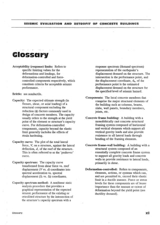
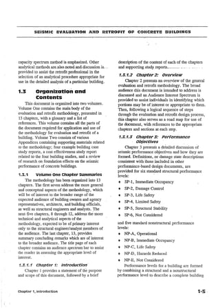
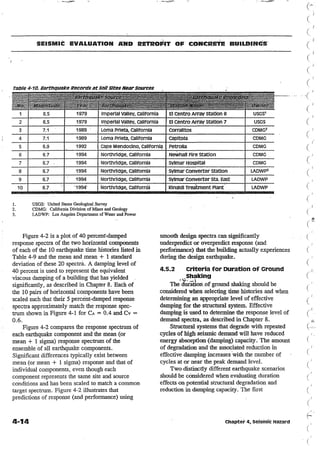
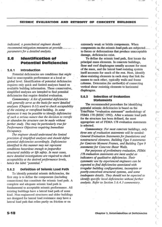
37. SEISMIC EVALUATION AND RETROFIT Oi= CONCRETE- BUH..DI.NGS
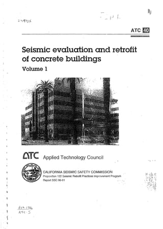
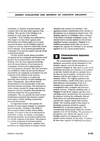
-·-----.,--Step by' Step ---S
R
A
T
E
G
y
C
0
N
C
E
p
IT]
~
~
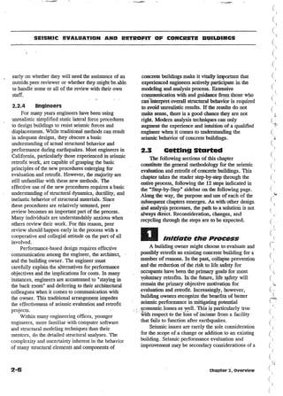
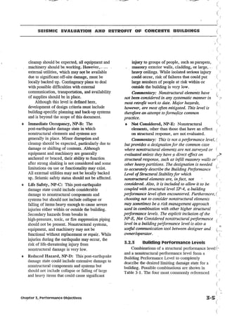
Select Qualified Professionals
Review Building Conditions
ffiJ
·ffiJ
L
'r 2, overview
Structural Engineer
Architect
Establish Performance Objectives
Structural Stability
Limited Safety
life Safety
D : f aControl
Imm . te Occupancy
Review Drawings
Visual Inspection
Prelininary Calculations
Formulate a Strategy
Simplified Procedures
Inelastic Capacity Methods
Complex Analyses
Begin the Approval Process
Building Official
Peer Review
[I]
~
Characterize Seismic Capacity
[[]
+ [9
D
E
[]
T
I
o
__.-
-- _.._...._
..
~
Chapters
Jurisdictional Requirements
Architectural Changes
Voluntary Upgrade
Conduct Detailed Investigations
T
A
~
~Pertinent
Initiate the process
[1]
T
- ..- _._-.'._ ....-..... _.. -_..
Site Analysis
Material Properties
Construction Details
Modeling Rules
Force and Displacement
Determine Seismic Demand
Seismic Hazard
Interdependence with Capacity
Target Displacement
Verify Performance
Global Response Limits
Component Acceptability
Conceptual Approval
Prepare Construction Documents
Similarity to New Construction
Plan Check
Form of Construction Contract
Monitor Construction Quality
Submittals, Tests, and Inspections
Verification of Existing Conditions
Construction Observation b Desi er
0
CB0
0CD
~
®:D
0:D
CD®§
0®
~
®:D
(2)
,.
,.
2·7

38. ~j~lr~~6J:l~~ ert;;;; un~n
(
for any
,
best" to follow a selection procedu, (sin
number .of reasons. Even if seismic performance...._:;+-- ---f.oll.owina: .
. ,
0
.
improvement is the primary motivation, it is wise
1. Generate a list of potentially qual.. I. «>
to consider a broader potential scope at the
candidates. This can be from past e. lerif
beginning ofthe project. Potential considerations
and general familiarity on the part ot
) 0.s
include the following:
or from references from others who ha 'if
similar projects. Public agencies' may dex lOp
• Fire and life safety improvements
request for qualifications announcement Wi .
• Hazardous material abatement
minimum criteria specified.
• Disabled ~ccess improvement
2. Request written submittals of statements of
• Change in programmatic use
qualifications. The request should state the
preliminary scope of the project to the extent
• Functional improvements
'. possible.
• BUildin~:~ysten;s improvements
3. Select several qualified candidates to submit
• Historic preservation
formal proposals; In some cases's available
Some of these are voluntary and may simply
drawings or other documents might be
make sense to include. Others may be required by
provided to the proposers. Site visits are also
law when changes are made to a building.
beneficial.
Jurisdictional requirements vary, and it is prudent
4. Interview one or more of thri cmdidates on the
to make conservative assumptions early in the
. I
basis of a review of the proposals. The
process. Theactual scope may not emerge until
interview is an opportunity to imagine the.
later in the project, when more information
working relationship between an owner and tl
becomes available. The expert advice of design
. potentialdesign team. Are the personalities
professionals, including an architect and an
compatible? Even if qualifications are
engineer, is normally needed to finalize the scope
excellent, the relationship between the owner
of a project. -Table 2-2 is a guideline to issues
and the consultants must also be -conducive tc
pertinent to the rehabilitation and retrofit process
success.
,
scope of work.
5. Thoroughly check references on similar
projects. Ask references specific questions
Slf!lect Quali#ied
about the performance of the candidates and
pJ:oFessiDntlls
about the results of the job:
Some owners have ongoing relationships with
6. Make a selection and negotiate acontract,
design professionals whom they know and trust.
Keep in mind that the scope may change on
Others may never have dealt with architects or
the' evaluation and retrofit strategy is
engineers. Public agencies are required to select
developed in the initial stages'of the projec
project teams-according to prescribed procedures.
This' selection process can be tailored to th
In any event, the careful selection of qualified
needs of individual projects. In most cases, at
professional assistance is more important with the
of design professionals led by either an archite
evaluation and retrofit of existing concrete
structural engineer is sought In some cases, a
buildings than with most other projects. This is
structural engineer might fill the role without
because of the complexity of the building type, the
architectural assistance. An example 'would be
uncertainties of earthquake technology, and the .
. _:,.~.}Vp"en. a; Pr.~limi:p.ary,',S~dYi to determine deficit
lack of establishedprecedents indesign and"
and develop conceptual remedial structural
analysis methodologies. Therefore, it is usually
Chapter 2,
OVE

39. SEISMIC EVALUATJON- AND -RETROFIT OF CONCRETE BUU.DINGS
Table 2-2. Seismic l!~sign (:hecklist fO Facilit;1t.e,l.;JrchitectiEngineer Interaction
structural stability
Limited safety {structural>
Hazards Reduced (non structurall
Life safety
structural
Nonstru ctural
Damagecontrol
Immediate tcontlnuern Occupancy
Continued post earthquake function
Near fault
Ground failure possibility [landslide,
liquefaction, subsidence) Soft soil (long periods, amplification,
duration)
vertical discontinuity
soft story
Setback
Offset
Resistance elements
Plan discontinuity
Adjacency-pounding possibility
Dynamic resonance
Diaphragm flexibility
Torsion
Redundancy
Deformation compatibility
out-of-plane vibration
Unbalanced resistance
Resistance location
Driftlinterstory effects
strong column/weak beam condition
structural performance
Ductility
Inelastic demand
Constant or degrading stiffness
Damping
Chapter 2,OVerviEiJw
i

40. (
(
,(
Table 2-2 (Continued) Seismic Design Checklist to Facilitate A,rChite.ct/e.ngineerInteraction
Energy dissipation capacttv
(
Yield/fracture behavior
-. (
special system (e.g., seismic Isolation)
(
Mixed system
Repairability
Up-slope or down-slope conditions,
collapse-hazard buildinQs nearby
(
Cladding, glazing
(
Deformation compatibility
Mounting system
(
Random infill
Accessibility <lifelines, access/egress)
Height
Size effect
Architectural concept
(
- .~;:.~
(
I
~
ceiling attachment
Partition attachment
Rigid
Floating
Replaceable partitions
stairs
Equipment (Mech.lElec}Plumb.l
(
special equipment
(
Computer/communications
equipment
I
(
special building contents
(
Source: Architectural Practice and Earthquake Hazards (CSSC 1992).
(
(
(
(
(
(
(
2-10
Chapter 2, overvieW
(
(
(
(:
~

41. measures is sufficient. An architect might be hired
later,. as.the situation dictatesc.ln.either.case, the....
qualifications of the structural engineer.are the
most pertinent to the seismic evaluation and
retrofit process. The key requirements are:
.. Demonstrated experience in the analysis,
design, and retrofit of concrete buildings in
seismically. hazardous regions
..
Basic familiarity with the principles of
performance-based seismic engineering and
design
..
Experience with inelastic analysis procedures
and thorough understanding of reinforced
concrete materials behavior
..
Fundamental grasp of structural dynamics and
the behavior of structures subject to strong
ground motion
+ Registration as a structural engineering
authority in California
There are some very qualified engineers in the
state who do not necessarily have all of the
credentials above. This does not mean that they
should be eliminated from consideration. An
example might be an engineer with a small
. .
practice who has a good working relationship with
a building owner. This individual might be
.
perfectly capable of coordinating and
implementing a fairly sophisticated evaluation and
retrofit design with the assistance of an expert
subconsultant with supplementary qualifications.
2~4
. Basic: Evaluntian nnd
Retrofit strategy
For the construction of anew project, the path
from start to finish is fairly clear from the
beginning. The owner has a good idea of what a
new building should be like, and with a little
advice, the cost is fairly easy to estimate.
However, the course of an existing building
evaluation and retrofit project is often very
different from that imagined at the outset. An
owner might have an idea about the desired
seismic performance, but rarely is it easy to
Chapter 2, overview
ascertain the .cost of attaining that level of
performanceearly.in, the. project. .The. architect.and
engineer are not starting with a clean slate as with
a new building. What are the strengths and
deficiencies of an existing building? How
compatible are these with the owner's objectives?
Is it worth while to spend a lot of money on
sophisticated analyses? Is it better for the owner
to simply accept the performance that can be
economically attained? These and other questions
can only be answered as the project unfolds.
Recognizing this at the start and planning a
flexible strategy to adjust to information as it
emerges are the keys to success.
.Establish PerFDrmance
Dbjec-cives
At 'the beginning of an evaluation 'project, the
design team should meet With the building owner
to discuss seismic performance objectives. These
are presented in detail in Chapter 3. Thepurpose
primary of these initial meetings is to review with
the owner the various options for seismic
performance. It is important to remember that
attaining a performance objective consists of
achieving a certain level of performance for a
specific level of seismic hazard. Chapter 4
contains a detailed treatment of seismic hazard
from ground shaking and addresses the potential
for ground displacement due to liquefaction,
surface faulting, and landsliding.
The consequences of earthquakes on buildings
can be categorized into three types of losses:
• Life Safety: deaths and injuries to building .occupants and passersby
+ Capital Losses: costs to repair or replace the
building or its contents
+ Functional Losses: loss of revenue or
increase in expenses related to the inability of
a facility to function normally after
earthquakes
2·11

42. -~~.
:
(
(
The level of performance for a building during.earthquakes is. measured.by, the.nature.and.extent ,.. .
of these potential losses. Obviously, the level of
performance is affected by the strength of each .
earthquake. It is reasonable to expect that a
building remain safe, i.e., not cause life loss, for
rare large earthquakes and that it remain usable for
more-frequent moderate events. A performance
objective is a goal that a building achieve a certain
level of performance for a specific level of seismic
ground shaking hazard. An owner might decide
that the goals for a 'building should' be to remain
life safe for the Maximum Earthquake hazard level
and functional after a Serviceability Earthquake'
hazard level event.
"
It is important that building owners understand,
that the process of seismic evaluation and-retrofit .
is a: risk-reduction process. The goals that owners
select for building performance are just "
that--goals. Qualified design professionals who
sense this Understanding in their. clients can be
extremely effective in helping owners to manage
risk and deal with uncertainty. They will be less
effective, on the other hand, for poorly informed
clients who try to transfer risk: and ,who expect
"guaranteed" building performance.
'
"_.,
Review Bunding
Conditions
Chapter 5 provides detailed guidelines for a
preliminary investigation' of a building by an
engineer. This process normally involves a site
visit to physically inspect the building and a search
for and review of existing drawings or other
documents that may describe the structural
characteristics of the building. The structural
engineer might also do some preliminary .
calculations to determine whether any of the
features of the building are potential seismic
deficiencies in terms of the preliminary
performance goals; Chapter 5 includes
recommendations on the types of information that
the engineer should compile. At this point, the
engineer should also consider the potential site
, hazards.covered. m-Chapter-4_-------- ---At some point during this initial process,
another meeting or series of meetings usually takes
place with the building 'owner, engineer, and
architect. On the basis "ofthe preliminary field
investigation, the engineer can often qualitatively
describe to the owner what it might take to meet
preliminary performance goals. In light of these
discussions, the owner and design team might .
decide to revise or augment the performance
objectives. For example, if a building owner is
initially interested only in life safety; the engineer
may be able' to determine from preliminary
investigations of the building that a performance
goal. beyond life safety could be achieved without a
much greater investment. Of course, in many ,
cases the opposite course must be taken: "
performance goals and expectations may have to
be lowered on the basis of what is determined in
the field. Supplemental detailed investigations of
existing conditions may be required at a later stage
in the process.
'
pc,mulelte'
(
(
(
(
(
(0
a stl'Dtegy
After the owner revises or confirms the
performance objectives, the design team should
develop a plan for the detailed evaluation and
possible retrofit. There are many possible
alternatives to mitigate seismic risks, as discussed
in Chapter 6. The owner should continue to
remain involved during this planning process.
This document presents relatively. new
technology that allows engineers to gain a more
realistic picture of the: potential seismic
performance characteristics of buildings. These
nonlinear static procedures constitute an inelastic
analysis that considers what happens to buildings
after they begin to crack and yield in response to
realistic earthquake motions. This approach differs
from traditional linear static procedures that
reduce seismic forces to levels that allow engineers
to design buildings under the assumption that they'
(
(
(
(
(
(u
Chapter '2, Overview
(
(
(

43. :
remain undamaged. Although unrealistic and
potentially misleading" this.simplistic.approach can,
work well for new buildings and for smaller,
simpler, and regular existing buildings. The
advantage of the newer, nonlinear static
procedures, when applied to existing buildings, is
that they credit the good features of buildings at
the same time that they identify deficiencies. In
spite of its improvements over traditional analysis,
this new approach may not be appropriate for all
buildings.
,
'
Some buildings may be too complex to rely on
the nonlinear static procedures. These cases may
require time history' analyses of the nonlinear
behavior of structures during example
earthquakes. The kinds of buildings that may
require these specialized analyses are those that
are highly irregular or complicated. Other
examples of building systems that may necessitate
more-sophisticated analysis are energy dissipation
or base isolation systems.
'
At the other end of the spectrum are simpler
buildings for which use of nonlinear static.analysis
is not necessary. Although there are no hard and
fast rules to identify them, buildings that possess
one or more of the following characteristics should
be considered candidates:
';
•
Small size
+ Low-rise (one or two stories)
•
Uncomplicated (regular) structural systems
+ Highly redundant lateral force resisting system
+ Low occupancy
For those cases, use of simpler, linear elastic
analysis procedures may be sufficient: There are a
number of such procedures, briefly reviewed in
Section 804.1, that may be utilized, depending on
the specific characteristics of-a given building.
In some cases, however, the simplified
procedures do not identify specific seismic
deficiencies. For example, in shear wall buildings
the columns can be subject to excessive
displacement and potentially fail when the shear
walls begin tocrack or rock at the foundation.
Chapter 2, overvie,:"
Simplified procedures generally will not identify
this deficiency, Simplified procedures can also
result in overly conservative designs. This is .
appropriate, since the level of detail required for
analysis in the simplified procedures is less
extensive than that for the more sophisticated
approach, so the additional conservatism is
warranted. In some cases, however, this additional
conservatism can result.in excessively high
construction costs. Also a consideration is the
.
.
potential for disruption and possible closure of
buildings for retrofit. The simplified procedures
tend to require more-extensive retrofits and are
more likely to cause disruption andlor the need for
vacating buildings.
Another situation where use of simplified
procedures is appropriate is when existing
structural systems are so inadequate that complete
new systems must be installed in any event. In this
case. the simplified procedure does not give up
much by neglecting the strength of existing .
systems. Also, if architectural considerations and
historical restrictions are not significant, the
freedom of placing resisting elements where they
are most effective can provide an opportunity for
simplified procedures. Furthermore, if a building
is highly redundant, not particularly irregular, and
of good construction quality, the scope of retrofit,
even if determined' by simplified procedures, is
likely to be small, and the benefits of moresophisticated analysis may be relatively
insignificant.
Simplified procedures have the advantage that
most engineers currently find them easier to use
than the new, nonlinear static procedures outlined
in this document. This is because the simplified
procedures more closely parallel the design
approaches that have traditionally been used in
structural engineering practice. It will take time
for engineers to assimilate the new procedures.
In addition, the simpler analysis procedures
lead to lower costs forevaluation and retrofit
design fees. In a competitive market, the lower
design cost approach is attractive to owners.
However, professional fees are not the critical cost
-~

44. (
(
(
(
(
consideration in seismic evaluation and retrofit. In
the long
-OFners_will.begin.to recognize rhe, ....
benefits of the better information obtained from'
use of the more sophisticated analysis procedures.
Better information leads to much-mere-significant
economy in the reduction of both construction
costs and actual earthquake losses.
run..:..
B~,gin
the Approval
Process
Once a plan for the evaluation of the building
is formulated, the basic strategy should be
reviewed in detail with the building official. This
sequence is somewhat different from that for .
traditional design and construction, where the
building official sometimes is not:consulted until
the end of the design process, The complexity and
uncertainty inherent in the seismic evaluation of
concrete buildings demand much greater
collaboration between the design team. and the
building official. At this point in the planning
process, the extent of the required peer review for
the project should be discussed. The scope of the
peer review depends on' a number of factors,
including the complexity of the building itself ana
the proposed. evaluation procedures, the ability of
the building department to understand and review
the evaluation and retrofit design, and the
capability and experience of the structural engineer
and design team. In most cases it is advisable to
. have a peer review panel. engaged early to evaluate
the strategy for the evaluation and retrofit. In some
instances, however, it may be acceptable to forego
formal peer review until the completion of the
evaluation and a conceptual design. Chapter 7
covers some of the more detailed aspects of the
peer review process and other quality control
measures.
CDnduce DetD/led
Investiga~iDns
The plan for the evaluation and retrofit process
often includes detailed tests and inspections to gain
more information about the specific characteristics
_of a particular building~[O.ne oLthe.reasOD..S.,.thaL_._ ....
..
careful planning and approval by all involved are
important in the early stages of the project is that .
these tests and inspections often can be expensive.
Some ofthe detailed options are reviewed in
ChapterS• .
In some cases the lack 'of drawings and other
documenration for a particular building may
significantly affect the selection of an evaluation
procedure. In fact, simplified procedures may be
most appropriate for buildings about which little is
known. In- these cases it often can be most costeffective to simply provide a completely new
seismic force resisting system rather than try to
thoroughly investigate and document existing conditions for more-sophisticated analyses.' .
The activities up to this point in the overall
evaluation of the retrofit process can beviewedas
a strategic planning effort. The complexity and
uncertainty involved in the overall process make
this stage extremely important in controlling both
the costs and the quality of the work: In some .
instances. the resulting plan may allow for .
contingencies and changes based on what is
discovered later 'on, For example, a nonlinear
static procedure may be considered' the most
effective analysis procedure in the beginning.
However, detailed investigations of field
conditions might lead to the conclusion that a
simplified analysis could economically satisfy the
performance- goals.
-.
2.5
Evaluation and Retr.ofit
con:cept _
'
.
(
(
(
(
(
C
(
(
(
(
e
(.
".
The essence of virtually all seismic evaluation
procedures is a comparison between some measure
of the "demand" that earthquakes place on a .
structure to a measure-of the "capacity" of the
building to resist. Traditional design procedures
characterize demand and capacity as forces. Base
shear (total horizontal force at the lowest level of
the building) is the normal-parameter that is used
for this purpose. The engineer calculates the' base
shear demand that would be generated by a given
(
(
I
(
(
(
(
( ;
2·14
("'
(
(

45. earthquake, or intensity of ground motion, and
demand to the capacity of a structure. This
compares.. this.to.the. base .shear-capacity .of.the. ._ _.- - -' --_.. approach..includes consideration-ofthe ductility of
..
building. The capacity of the building is an
the structure on an element by element basis. The
estimate of a base shear that would be
inelastic capacity of a.building is then a measure
of its ability to dissipate earthquake energy. The
"acceptable." If the building were subjected to a
force equal to its base shear capacity some
current trend in seismic analysis is toward these
deformation and yielding might occur in some
simplified inelastic procedures. Chapter 8 is a
detailed presentation of how they are used to
structural elements, but the building would not
collapse or reach an otherwise undesirable overall
compare the capacity of a structure to the demand
level of damage. If the demand generated by the
imposed on it by a given ground motion.
earthquake is less than 'the capacity then the design
is deemed acceptable.
The first formal seismic design procedures
Characterize seismic
recognized that the earthquake accelerations would .
capacity
generate forces proportional to the weight of the
The recommended central methodology in this
building. 'Over the years empirical knowledge
document concentrates on the formulation of the
about the actual behavior of real structures in ,
inelastic capacity curve for the structure as
earthquakes and theoretical understanding of
presented in Chapter 8. This curve is a plot of the
structural, dynamics advanced. The basic procedure
horizontal movement of a structure as it is pushed
was modified to reflect the fact that the demand
to one side. Initially the plot is a straight line as
generated by the earthquake accelerations was also
the structure moves linearly. As the parts of the
a function of the stiffness of the structure.
structure yield the plot begins to curve as the
Engineers also began to recognize the
structure softens. The engineer generates this
inherently better behavior of some buildings over
curve by building a model of the entire, structure
others. Consequently, they reduced seismic
from nonlinear representations of all of its
demand based on the characteristics of the basic
elements and components. Most often this is.
structuralmaterial and systein. The motivation to
accomplished with a computer and structural
reduce seismic demand for design came because
analysis software. Using-the modeling rules of
engineers could not rationalize theoretically how
Chapters 9 and 10 the engineer specifies force
structures resisted the forces generated by
and displacement characteristics for each piece of
earthquakes. This was partially the result of their
the structure resisting the earthquake demand.
fundamental assumption that structures resisted
These pieces are assembled geometrically to
loads linearly without yielding or permanent
represent the complete lateral load resisting
structural, deformation.
system. The resulting model is then subject to
An important measure-the capacity of a
increasing increments of load in a pattern .
structure to resist seismic demand-is aproperty
determined by its dynamic properties. The '
known as ductility. Ductility is the ability to
corresponding displacements define the inelastic
deform beyond initial yielding without failing
capacity curve for the building. The generation of
abruptly. If a pencil is bent up to and beyond its
the capacity curve defines the capacity of the
yield point, it snaps. In contrast, a coat hanger
building uniquely and independently of any
deforms permanently way beyond its initial yield.
specific seismic demand. In this sense, it replaces
It is ductile compared to the pencil. This property
the base shear capacity of traditional procedures.
is a critical component of structural capacity.
Instead of comparing forces, nonlinear static
procedures use displacements to compare seismic
EI
t.,
Chapter 2, Overview

46. -.-.~,
(
(
(
SEISMIC EVAl.UATION AND RETROFIT' OF COrn:RETE BUILDINGS
":1
Evolution of Seismic De~ign
+f- d
Earthquake
Displacement
v
Lack of Knowledge
on Earthquake
Demand and
Building Capacity
Historical Approach
Earthquake forces proportional to
building mass
'(V des =5-10% of WL),
(
(
(
(
• Linear design using "factors-of
, safety" to account for uncertainty
- iu earthquake, pemand and
building capacity
Traditional Code Basis
v
Elastic earthquake forces reduced for
linear design _
(V d..
=V
max.
I R)
(
R. varies based' on typical inelastic
response of structural types
Reduction justified by expected
11 IDOX I 11 yield
ductility,
Inelastic
Response
(
tJ.
yield
, Current Trend
Inelastic earthquake demand based on,
inelastic capacity of building
Resolution of demand vs, capacity
generates Performance Point
Sa
Demand Reduced Based
on Inelastic Capacity
(
-
_---tIl::--m--~m1mng
l
(
• Design based on displacement,
A des
I
(
(
I
(
(
(
(
Chapter 2, overview
(
(
(
'.

47. !3EISMI't .EVALUATI.ON AND RETROFIT OF CONCRETE BUILDINGS'
::
case as most analyses include some inelastic
nonlinear behavior. _.. .
To find the point where demand and capacity
are equal, the engineer assumes a point on the
capac~ty spe.ctrum as an initial estimate. Using the
spectral acceleration and displacement from this
point, the engineer then can calculate reduction
factors to apply to the 5 ~ elastic spectrum to
account for the hysteretic energy dissipation
associated with the .specific point. These reduction
factors have the effect of pulling the demand
spectrum down. If the reduced demand spectrum
intersects the capacity spectrum at or near the
initial assumed point, then it is the .solution for the
unique "performance point" where capacity equals
demand. If the intersection is not reasonably close
to the initial point, then the engineer can assume a
new point somewhere between and repeat the
process until a solution for the performance point
is reached.
Chapter 8 also presents an alternative for
estimating the "performance point" where capacity
and demand all equal for a given earthquake
motion. The proposed federal guidelines (ATC,
1996a) presents one of these called the
Displacement Coefficient Method. It uses a series
of coefficients to modify the hypothetical elastic
response of a building to estimate its inelastic
displacement demand.
When an earthquake displaces the building
laterally,..its..response is represented bya..point.on
this curve. A point on the curve defmes a specific
damage state for the building, since the
deformation of all of its components can be related.
to the global displacement of the structure.
~
Determine seismic:
. . . Demand
The capacity of a particular buildirig and the
demand imposed upon it by a given earthquake
motion are not independent. One source of this
mutual dependence is evident from the capacity
curve itself. As the demand increases the structure
eventually yields and, as its stiffness decreases, its
period lengthens. Conversion of the capacity curve
to spectral ordinates (ADRS) outlined in Chapter
8 makes this concept easy to visualize. Since the
seismic accelerations depend on period, demand
also changes as the structure yields. Another
source of mutual dependence between capacity and
demand is effective damping. As a building yields
in response to seismic demand it dissipates energy
with hysteretic damping. Buildings that have large,
stable hysteresis loops during cyclic yielding
dissipate more than those with pinched loops
caused by degradation of strength and stiffness.
Since the energy that is dissipated need not.be
stored in the structure, the damping has the effect
of diminishing displacement demand.
Chapter 8 devotes much attention to the
development and presentation of the Capacity
Spectrum Method. The Capacity Spectrum Method
characterizes seismic demand initially using a 5 %
damped elastic response spectrum as detailed in
Chapter 4. This spectrum is plotted in spectral
ordinates (ADRS) format showing the spectral
acceleration as a function of spectral displacement.
This format allows the demand spectrum to be
"overlaid" on the capacity spectrum for the
building. The intersection of the demand and . ' , " 1
capacity spectra, if located in the linear range of
the capacity, would define the actual displacement
for the structure; however this is not normally the
Chapter 2, ove~view
·m
,..,.,.
Verify Performance
Once the performance point for a demand
earthquake is estimated, the engineer checks the
resulting performance of the building using the
. acceptability criteria in Chapters 10 and 11. The
performance is checked on two levels. First, there
are global-limits for displacement of the structure
for each performance objective. For example, the
roof of a building might move four inches during
an earthquake for· which it should be life safe. For
the same building the total roof displacement
might be limited to two inches for a more frequent
earthquake in order to meet a damage control

48. -~ -- -'--:--~.
(,
(
(
(
(
(
(
:
(
(
(
.
.Capacity-vs: -D'emaricf-c---------------.:-------.
.
(
(
(
(
~~
('
C.
(
(
(
S
a
(
T
'
(~
/Ra:uced
seismic
demand
(
(
(
Performance
point
,
(
(
(
(
(
(
(
(
(
,
Chapter 2, overview
(
(

49. SEISMIC EVALUAY·ION AND RETROFIT OF CONCRETE EUULDINCS
the engineer can pinpoint deficiencies within the
performance goal. Similarly, the. engineer checks
individual. structural elements.against acceptability.. :_- ... structure., This.facilitates.a.directed retrofit. strategy.
limits which depend on the global performance
that is both effective and cost efficient.
goal. The nature of the element acceptability limits
In order to meet some or all of the performance
vary according to the specific element. Inelastic'
goals for abuilding, retrofit may be required to
rotation is the acceptability parameter for beams,
improve performance. If the performance goals are
for example. The limits on inelastic. rotation are .
met by the existing structure then retrofit may not
recommended based on observations from tests and
be necessary. There are several strategies to
performance in past earthquakes. A similar, though
develop appropriate retrofit measures as discussed
somewhat more qualitative procedure measures the .
in Chapter 6. The choice depends on the type of
acceptability. of nonstructural components.
structure, the nature of the deficiencies, the
The nonlinear static procedures, including the
constraints of the architecture and planning, and the
Capacity Spectrum Method, can appear to some to
funds available. In some cases, the owner may
be tedious and complicated compared to. traditional
decide to accept lesser performance in deference to
design procedures. There are, however, some
these constraints. The effectiveness of a selected
distinct benefits.
retrofit strategy is tested by adding or modifying
First, the entire process of generating the
elements in the structural model, then re-analyzing
capacity curve and dealing directly with the
the model as before. Often several different
interdependence of capacity and demand gives the
strategies are investigated before settling on a
engineer a greatly enhanced understanding of the
preferred concept.
actual performance of the specific building. This
enables the engineer to apply the necessary
2 ..&
Fingl Design and
experience and judgment at a much more refmed
construction
level than traditional procedures.
This document concentrates on the conceptual
Also advantageous are the significantly more
phase of seismic evaluation and retrofit projects. In
useful results of the analysis. The performance
reality, the detailed design work represents a major
point at which the seismic capacity equals the
portion of the effort and occurs after the owner's
demand characterizes performance as a specific
preferred concept is developed. This process,
building damage state for a specific earthquake
however, is similar to that for conventional'
intensity. The probability of occurrence of the
construction of new buildings.
earthquake intensity defines the risk of occurrence
for the damage state.
Although the accuracy of this estimate is limited
Prepare Construction
by unavoidable uncertainties, this explicit
Documeni:s
relationship between performance and risk is
superior to the implicit intent of current code
The structural details for the retrofit typically
procedures. Component deformations, directly
conform to code requirements for new work. As the
related to damage, are a much better parameter than
design continues, the peer reviewer checks to see
forces for performance evaluation. In contrast to
that the approved concept is faithfully implemented
force-based traditional methods, the damage state
by the engineer, as discussed in Chapter 7. These
from nonlinear static procedures characterizes the
reviews usually occur at the end of the design
deformation of building components for comparison
development phase and near the completion of
with acceptability criteria depending on the desired
construction documents. Before issuing a permit for
performance. With the tabulation of the
construction, the building official will normally
acceptability of individual element deformations,
have a plan check made of all project documents.
>.
m
Chapter 2, overview

50. (
(
((
(
(
(
:
In the absence of legal restrictions, the form of
.contract for retrofitconstruction.may be. one. oL....
many, similar to new construction. Lump sum
bidding is best suited to projects where the existing
conditions of the building are relatively welllmown
and the retrofit measures comprise. normal
construction practices. Where field conditions are
uncertain or retrofit measures are innovative or
unique, a construction management approach can be
very effective. In fact, engaging a contractor during
design can often provide valuable assistance to the
engineer, in the selection of cost-efficient retrofit
techniques and details of construction. A unique
contractual arrangement. may be appropriate- in
some cases--for instance, where there are
specialized retrofit procedures, such as seismic
isolation or energy dissipation devices.
.
.
"j
-
;
·
m
,!,~n1..t~1' conse,uction,
-l,1u~/'ty·-------------
The actual seismic performance of buildings is
extremely sensitive to construction quality. This is
especially true for .retrofitted buildings. Field
conditions in existing buildings routinely vary from
those shown on drawings or implied by visual
inspections during the evaluation process. These
changes can,have significant impact on retrofit
designs. Some retrofit techniques are sophisticated
~d require special inspections and tests. It is vitally
Important that the engineer prepare a projectspecific construction quality assurance plan. The
plan should identify required jests, inspections,
submittals, and personnel qualifications. The
engineer of record should make. regular inspections
and receive immediate .notification of any field
problems,
._....
(
(
(
(
.(
(.
'f
(
(
(
(
(
(
(
(
(
(
(
(
(
(
(
(
(
(
(
2-20
Chapter i~ overview
(
(

51. .:
building performance levels are given titles and are
escribed.below.
,., ",.,._._. ., .... _ ....
.., ,.,
Commentary: The four building performance
.vels; Operational, Immediate Occupancy, Life
~afety, and Structural Stability; are 'given' titles
.onsistent with the titles of their structural and
-mstructural components. Reference can also be
made to their SP-NP designations, I-A, I-B, 3-C.
-id5-E. Rather than developing titles for all other
combinations, some of whicb will seldom be
- nployed, it is recommended that the SP-NP
designations be used.
... Operational, I-A: This is the performance
level related to functionality. Damage to the
building's structure is limited so that continued
safe occupancy is not in question, and any
required repairs are minor and can be carried
out without significant disruption to occupants.
Similarly, damage to nonstructural systems and
contents related to functionality is minor and
will not jeopardize functions in the building.
'Most importantly, vital servicesfrom outside
the building such as utilities, transportation, or
communications must be provided withback-up
facilities or planning as required to allow
functions to continue if these services are
unavailable. Since important aspects of this
performance objective involve contingency
planning and design of back-up systems,
development of acceptability criteria is not
included in this document.
Immediate Occupancy, I-B: This corresponds
to the most widely used criteria for essential
facilities. The building's spaces and systems are
expected to be reasonably usable, but continuity
of all services, either primary or backup, is not
necessarily provided. Contents may be
damaged.
Commentary: Although most codes require
jairly complete and effective seismic anchorage and
tacing for building systems and equipment, the
actual operational aspects of a facility are normally
tveloped by the owner-operator. Although some
operational aspects, such as requirements for more
complete back-up utility systems could be put in
codes.fot.use.of.building.designeis.Jt. may.not... be _
practical to attain an Operational building ,
performance level without significant
facility-specific input from the owner-operator.
+ Life Safety, 3-C: This level is intended to
achieve a damage state that presents an
extremely low probability of threats to life
safety, either from structural damage or from
falfug or tipping of nonstructural building
components. User-furnished contents,
however, ar:e not controlled, and could create
falling hazards or secondary hazards, such as
chemical releases or fire. This performance
level is intended to be less than 'the
performance that is expected of code designed
new buildings.
+ Structural Stability, 5-E:
This damage state
addresses only the main building frame or
vertic~ load carrying system arid requires only
stabi.Iji:y under vertical loads.. No margin
against collapse in aftershocks may be
. available. Life threatening external or internal
falling hazards from cladding,' nonstructural
finishes, or 'even structuraldamage may have
occurred. Review of performance of
nonstructural elements from' expected forces or
structural 'drifts is not required so their
performance can be' highly unreliable,
+ Other Commonly Used 'Combinations
o
Building Performance Level 3-D: This
level combines life safety structural
performance with the reduced hazard
nonstructural performance, thus accepting
a slight risk to life safety from
nonstructural systems. Although large and
highly vulnerable nonstructural elements
should remain in place, the majority of
nonstructural elements such as
mechanical/electrical equipment and
distribution systems, partitions, and typical
.
,
,
chclpter 3, Performance Objectives

52. (
(
(
-----------------------------------------_
(
(
(
cleanup should be expected, all equipment and
.machinery. should.be..working; Ho;wever,--.-external utilities, which may not be available
due to significant off-site damage, .must be
locally backed up. Contingency plans to deal
with possible difficulties with external
communication, transportation, and availability
of supplies should be in place.
Although this level is defined here,
development of design criteria must include
building-specific planning and back-up systems
and is beyond the scope of this document.
..
Immediate Occupancy, NP-B: The
post-earthquake damage state in which
nonstructural elements and systems are
generally in place. Minor disruption and
cleanup should be expected, particularly due to
damage or shifting of contents. Although
equipment and machinery are generally
anchored or braced, their ability to function.
after strong shaking is not considered and some
limitations on use or functionality may exist.
All external utilities may not be locally backed
up. Seismic safety status should not be affected.
+- Life Safety, NP-C:. This post-earthquake
damage state could include considerable
damage to nonstructural components and
systems but should not include collapse or
falling of items heavy enough to cause severe
injuries either within or outside the building.
Secondary hazards from breaks in
high-pressure, toxic, or fire suppression piping
should not be present. Nonstructural systems,
equipment, and machinery may not be
functional without replacement or repair. While
injuries during the earthquake may occur, the
risk of life-threatening injury from
nonstructural damage is very low.
..
Reduced Hazard, NP-D: Thispost-earthquake
damage state could include extensive damage to
nonstructural components and systems but
should not include collapse or falling of large
and heavy items that could cause significant
injury to groups of people, such as parapets,
masonry. exterior walls, .cladding,..or large, -. (
heavy ceilings. While isolated serious injury
(
could occur, risk of failures that could put
(
((
large numbers of people at risk within or
outside the building is very low.
Commentary: Nonstructural elements have
not been considered in any systematic manner in
most retrofit work to date. Major hazards,
however, are most often mitigated. This level is
(
therefore an attempt to formalize common
practice.
• Not Considered, NP-E: Nonstructural
elements, other than those -that have an effect (
on structural response, are not.evaluated.
Commentary: This is not a performance level, (
but provides a designation for the common case
where nonstructural elements.are not surveyed or (
(",I.r=
evaluated unless theyhave .fJ. direct effect on
structural response, such as infill masonry walls or
'.
other heavy partitions. The. designation is needed
to accurately describe the Building Performance
Level of Structural Stability for which
(
nonstruetural elements are; in fact, not
considered. Also, it is included to allow it to be. (
coupled with structural level SP-4, a building
performance level often encountered. Furthermore, (
choosing not to consider nonstructural elements
may sometimes be a risk management approach
used in combination with other higher structural
performance levels. The explicit inclusion of the
NP-E, plot Considered nonstructural performance (
level in a building performance level is also a
useful communication tool between designer and
owner/operator.
(
3.2.3
Building Performance Levels
(
Combinations of a structural performance level
and a nonstructural performance level form a
(
Building Performance Level to completely
describe the desired limiting damage state for a .
(
building. Possible combinations are shown in
Table 3-1. The four most commonly referenced
(
(
Ch~Pter
3,
,performan~e
Objectives
3=5· .
(
(
~"

53. SEISMIC EVALUATION AND RETROFIT
OF'
COlNCR'ETE" BUILDINGS'
for the situation where a 'retrofit may not meet
done with caution, as this could imply a high
..all.the.structural.requirements of the, Life_ Safety__ .
. pr..obabililjLojcollapse.fotany.larget: event. __.. _.-:-~_. __.
level, but is better than the level of Structural
.. Not Considered, SP-6; This 'is not a
Stability. These circumstances include cases
performance levekbut provides ~ placeholder
when the complete Life Safety level is not-cost
for situations where only nonstructural seismic
effective, or when only some critical structural
evaluation or retrofit is..performed:
.deficiencies are mitigated
Commentary: Although. unusual,
(The nonstructural performance level used in
nonstruetural seismic improvements are sometimes
this .range varies and will depend on the intent
made with no review of the structure. This might
of the damage control).
. .' occur in locations ofhigh and obvious
I
Structural Stability, SP-5: This level is the
vulnerability, such as at a computer room or for
lirni ting post-earthquake structural damage state.
important equipment. The explicit inclusion of a
in which the' building's structural system is on
Not Considered structuralperformance level in the
the verge of experiencing partial or total
building performance level-is also useful
collapse" Substantial damage to the structure
communication tool between designer and 'owner. .
has occurred,: potentially including significant
3.2.2
Nonstructural Performance
degradation"hi the stiffness and strength of the
Levels
lateral force resisting-system. However, all
significant components of the gravity load
Nonstructural performance levels are assigned
resisting 'system continue to -carry their gravity
a title and, for ease of reference; a letter. The
demands. Although thebuilding retains its
letter is called the nonstructural performance letter
and is abbreviated NP-n (where n is the designated
overall' stability, significant risk of injury due to
.
falling hazards may exist both within and.._ .', -: ';>;!~.tteJ;"j'. -,;,~ ·~:,;r;.' .
outside the building and significant aftershocks
., The nonstructural performance levels 'may lead to collapse. It should be expected that
Operational, Immediate Occupancy, Life Safety ~
significant major structural repair will be
and Hazards Reduced -. are discrete damage states
and can be used directly in evaluation and retrofit
necessary prior to reoccupancy .. In the older
procedures to define technical criteria. ·The other
concrete building types considered in this
document, it is very likely that the damage will
nonstructural performance designation - Not
not be technically or economically repairable.
Considered - is an important placeholder to allow
Falling' hazards are not specifically
direct reference to the wide variety 'of building:
prevented to achieve this performance level.
performance levels that 'might be desirable to
Therefore NP-E (nonstructural performance not
owners for evaluation or retrofit.
considered) is normally combined with SP-5.
Commentary: Performance levels have been
Commentary: This level is provided primarily
selected to allow combinations with structural"
o enable a specific verification of continued
levels that will correspond to single performance
levels proposed by FEMA 273 and Vision 2000 and
structural stability for the maximum earthquake
jround motions. Although such performance is
provide the flexibility to formalize de facto
" implied (SEAOC 1990) for new buildings in
combined performance-levels commonly used in
Ealifomia, and is considered desirable in all
practice.
seismic regions, there has previously been no
.. Operational, NP-A: The post-earthquake
J ormalized method of verification. The combination
damage state in which nonstructural elements
,t this structural performance level with earthquake
and systems are generally in place
ground shaking less than the maximum should be
functional. Although 'minor disruption and
a
and
3-4
Chapter 3, performance 'Objectives

54. -
-,"",--,"=",,""'
---
t
(
(
(
(
:
{
(
(
(
are similar to those used in FEMA 273 (ATC
reparability is so undefined that the term is no
1996a) .. These descriptions are.also.similar in__
. _.mor.e..u.sefuLthan.Damage-Contr.oLIL is expected
concept, if not in terminology, to those proposed in
that many projects may have special demands for
the Vision 2000 Progress Report (SEAOC 1995b).
which criteria greater than Life Safety will be
appropriate. Although not a level, per se, it is far
.. Immediate Occupancy, SP-l: The
simpler to reference this range ofperformance
post-earthquake damage state in which only
levels using a placeholder. within the context of
very limited structural damage has occurred.
standard designations (e.g. SP-2) than to formally
The basic vertical and lateral force resisting
define both levels and ranges.
systems of the building retain nearly all of their .
pre-earthquake characteristics and capacities.
.. Life Safety, SP-3: The post-earthquake
The risk of life-threatening injury from
damage state in which significant damage to
structural failure
.
the structure
is negligible, and
may have
the building'
occurred but in
should be safe for"
which some
unlimited egress,
margin against
ingress, and
. either total or
occupancy.
partial
structural
.. Damage Control,
collapse
SP-2: This term
remains, The'
is actually not a
level of damage
specific level but
is lower than
a range of
that- for the
post-earthquake
Structural
damage states that
Stability level. Major structural components
could vary from SP-I, Immediate Occupancy to
have not become dislodged and fallen,
SP-3, Life Safety. It provides a placeholder for
threatening life safety either within or outside
the many situations where it may be desirable
the building. While injuries during the
to limit structural damage beyond the Life
earthquake may occur, the risk of
Safety level, but occupancy is not the issue.
life-threatening injury from structural damage
Examples of damage control include protection
is very low. It should be expected that
of significant architectural features of historic
extensive structural repairs will likely be
buildings or valuable contents.
necessary prior to reoccupation of the
Commentary: The Damage Control range, also
building, although the damage may not always
sometimes called Limited Damage, is' defined to .
be economically repairable. This level of
allow reference to performance levels between
structural performance is intended to be less
Immediate Occupancy and Life Safety. Although not.
than the level of performance expected of fully
specifically defined in other current documents, the
code compliant new buildings.
expected performance of most new buildings for the
+- Limited Safety, SP-4: This term is actually
10 percent/50-year event (see Section 3.3) would
not a specific level but a range of
probably fall in this range (EERI 1994). A
post-earthquake damage states that are less
performance equivalent to that expected of new
than SP-3, Life Safety and better than SP-5 ,
buildings is also sometimes called Repairable
Structural Stability. It provides a placeholder
Damage, but economic or technological
Chapter 3,
Perform~nce
(
(
(
(c
(
(
(
(
(
~
~
(
(
(
(
Qbjectives
(
..

55. SEISMIC EVALU'ATioN AN'D RETROFIT OF CONCRETE' BUILDINGS
:
-able ~-1. Combinations of structural and Nonstructural perFormance Levels
to Form Building PerFormance Levels ,
)' .:;
,~, "
I
NP-A
operational
NP-B
Immediate
occupancy
~
Is,
•
NP-C
Life Safety
NP-D
Hazards
Reduced
NP-E
Not consloereo
Legend
Commonly referenced Building Performance Levels (SP-NP)
Other possible combinations of SP-NP
Not recommended combinations of SP-NP
~ombination of
a structural performance level and a
uonstructural performance level and are designated
'lY the applicable number and letter combination
such as I-A, 3-C, etc. as shown in-Table 3-1.
'.
,
';.2.1
~
structural perform~i;'ce Levels
and Ranges
Structural performance levels and ranges are
.ssigned a title and, for ease of reference, a
number. The number is called the structural
~L)erformance numberand is abbreviated SP-n
(where n is the designated number).
"-'
I
The Structural Performance LevelsImmediate Occupancy, Lif6 Safety, and Structural .
Stability-are discrete damage states, and can ,be
used directly in evaluation ,3.Pd retrofit procedures
. t~"defui~techJiiGafcnteiia': The other structural
performance designations-Damage Control,
Limited Safety, and Not Considered-are
important placeholders in the numbering scheme to
allow direct reference to the wide variety of
building performance levels that might be
desirable to owners for evaluation or retrofit.
Commentary: These descriptions of
acceptable damage at various performance levels

56. ---------------------------------------
(
(
(
(
(
(
Chapter :5
. .
___ .
~
.__.c_.
~~.f-c;J r·~~,~_~~_~~"j_~~tiJl.
~
._ _ ~_~__ _;_"'-----'-~.-. __ ~_.
~
(
s_
~__....
J
..._ c__~_..
._-----------/
,.-
,/f
AUdience
, Owner
Architect'
(
Interest spectrum
BIC/g. Official
. Engineer
Analvst
-.
3..1
Introduction
A performance objective specifies the desired
seismic performance of the,building: Seismic '
performance is described by designating the
maximum allowable damage state (performance
level) for an identified seismic hazard (earthquake
ground motion). A performance objective may
include consideration of damage states for several
levels of ground motion and would then be termed
a dual- or multiple-level performance objective.
Once the building .owner selects a performance
objective, the engineer can identify the seismic
demand to be used in the analysis and the
acceptability criteria
to be used for
evaluation and
design of the
building's structural
and nonstructural
systems. While the
majority of
retrofitted buildings
are expected to meet
or exceed the
assigned
performance level-when exposed to the ground
motion implied by the selected hazard level, such
performance should not be considered guaranteed.
This chapter defmes several standard
performance levels for structural and nonstructural
(
BII C
systems and several commonly used combinations (
of structural and nonstructurallevels, called
(
Building Performance Levels. Standard earthquake
hazard levels are introduced and the process of
(
selecting appropriate performance objectives is
described. A detailed discussion of seismic hazard
is contained in Chapter 4,"
(
3 ..2
Performance Levels
A performance level describes a limiting
. damage condition: which may be considered
satisfactory for a given building and a given
ground motion. The limiting condition is described
by the physical damage
within the building, the
threat to life safety of the
building's occupants
created by the damage, and
the post-earthquake
serviceability of the
building.
Target performance
levels for structural and
nonstructural systems are
specified independently"
Structural performance levels are given names and
number designations, while nonstructural
performance levels are given names and letter
designations, Building Performance Levels are a
(
(
(
(
(
(
(
(
(
(
(
Chapter 3, perforlt!anCe Objectives
'"

57. .•··;rio:,r.·.,.
., . . . .
SEISMIC EVALUATION AND RETROFIT 0;: CONCRETE BUILDINGS
Building Performance Levels 2-A, 2-B,
-- ---' 2-C,-2-D:.-Within- the broad structural- .
ceilings and light fixtures have not been
braced.or. anchored.and.could. be.highly...
disrupted and produce falling hazards.
It
performance range of Damage Control, an
equally wide range of nonstructural
protection might be appropriate. It is
unlikely, but possible, to find it desirable
to combine structural Damage Control
with less thorough nonstructural protection
than NP-C. It is necessary to develop
building specific criteria for these cases to
suit the systems needing special protection.
Commentary: The vast majority of all retrofits
completed to date have been designed to provide
performance similar to this level for the code
prescribed 10 percent/50 year earthquake ground
motion. A common design criteria has incorporated
75% of the lateral force required for new buildings.
Although most of these retrofits were designed to
prescriptive provisions and were therefore not
performance based, the intent was to achieve
structural life safety, and included mitigation of
major and obvious falling hazards such as parapets
or heavy decorative ceiling in large rooms.
Extensive surveys of other nonstructural elements
rarely have been included.
II
building code requirements for new
buildings is generally thought to be
intended to provide seismic performance
similar to Performance Level 2C for the
10 percent/50 years ground motion.
Building Performance Level 3-B: This
level presents a risk of structural damage
Qa
that could prevent the building from being
occupied. However, nearly complete
nonstructural protection will prevent .
significant internal disruption, particularly
in low levels of shaking. Although only
seldom applied to a whole building, this
level is more commonly applied to
.
particular areas or rooms, such as computer l
facilities.
e
•
8
chapter :3, Per.formance Objectives
Building Performance Levels 5-C, 5-D,
6-C,6-D: 1-1 some cases, improved
nonstructural performance may be
desirable with little or no consideration of
structural performance. As mentioned
previously, use of the SP-NP designation
forces recognition of structural risks when
such decisions are made.
Building Performance Level l-C: This
combination might represent the desire to
avoid a red or yellow tag structurally, but
the willingness to accept considerable
cleanup before the building's spaces are
fully usable. (It is unlikely that SP-l would
be combined with less than NP-C.
Building Performance Levels 4-C, 4-D,
4-E: Similar to SP-4, these levels are
primarily placeholders for structural risk
. reduction that does not meet a
predescribed level. A variety of
nonstructural improvements may also be
made.
Other Less Common Combinations
II
Building Performance Level 3-E: This
. level might be used if structural work is
minor or localized, or if limited funding
precludes expenditures for extensive
nonstructural upgrading.
Commentary: Building Performance Level 3-B
might be assigned to buildings where occupancy
and/or function is important, but the cost of
providing more structural protection is high, or if
the structure already meets the Life Safety
performance level. In these cases, structural work
may be extremely undesirable, but added
nonstructural protection is judged cost effective.
•
Building Performance LeveI3-A: This
•
Not Recommended Combinations: Certain
combinations of structural and nonstructural
performance levels will seldom, if ever, be
cost effective because of an imbalance in effort
on structural and nonstructural systems. Such
imbalances may also create rnisperceptions of

58. (
.(
(
(
(
SEISMIC EVALUATION AND RETROFIT OF CONCRETE BUILDINGS
(
(
.l
(
I
(
expectations by owners or tenants. Although
assignment of these,building,performance.levels
is not prohibited, the· Not Recorrunended
designation was addedboth to avoid poor
decisions and to simplify Table 3-1.
3.3
Earthquake·Ground
Motion
Earthquake ground motion is combined with a
desired performance !e:vel to form a performance
objective. The earthquake ground motion can be
expressed either by
specifying a level of
shaking associated with a
given probability of
occurrence (a
probabilistic approach),
.'
or in terms of the
maximum shaking
expected from a single
event of a specified
magnitude on a specified
source fault (a
deterministic approach).
The level of ground
motion is expressed in
terms of engineering
characteristics' for use in
design, A response spectra or an equivalent series
of simulated recordings of earthquake motions are
used for this purpose. .
The following three levels of earthquake ground
motion are defined in Chapter 4. .
.. The Serviceability Earthquake (SE): Ground
motion with a 50 percent chance of being
exceeded in a 50-year period
.
..
..
The Design Earthquake (DE): Ground motion
with a 10 percent chance of being exceeded in a
50-year period
The Maximum Earthquake (ME): Maximum
level of ground motion expected within the
known geologic framework due to a specified
single' event (median attenuation), or the ground
motion with a 5 percent chance of being
.-.exceeded.in.a5.Q.,-ye.a.r.period: _ .
__
_.
Commentary: The ground motion with-a 20
percent chance of being exceeded in 50 ye'!rs has
also been used in some projects. This ground
··lft(jtiontypicallyrepresentsabrJutlWlFthir~w···· .
-three-quarters ofthe demand ofthe more standardDE of10 percent/50 years. This reduced seismic
demand is roughly equivalent to the lower design
force level often used in the past for evaluation
and retrofit of existing buildings, e.g., ATC-14
. (ATC 1981), FEMA 178
(BSSC 1992), the San
Francisco Building
. Code Section- 104f
(City and County of San
Francisco 1991).
. Although the
" recommended system of
creating and assigning
performance objectives
allows and encourages
use 'of many levels of
performance and'
, ground motions, a
.' . common measure is
" needed to ;enable
comparison of
performance objectives with that expectedfrom
familiar designs, such as new buildings. The most
common and consistent thread for designs for the
last 20 years is the 10 percent/50 years ground
motion and it is recommended that this motion be
maintained for the basic Design Earthquake.
Lower criteria that have often been used for
existing building, usually in consideration- of the
high cost of retrofit, should be taken'into. account
directly by setting appropriate peif0T17ll!:'!oce levels.
As noted earlier, the Life Safety Performance Level
is intended to be a lesser criteria than the code for
new buildings and to accomplish a purpose similar
to the use of smaller design forces. However, with
performance based design, it is hoped that
communication of expectations to owners and
tenants will be inore straightforward.
(
I
(
(
(
I
r
C
(
(
(
(
(
(
(
(
(
(
(
(
(
(
(
I
I
(
(
(
(
~ ..
(
(
(
(
(
(
(
3-B
(
(
-,

59. SEISMIC .EVALUAT·IDN AND RETROFIT. OF CONCRETE BUU.DINGS
:
3.4
Performance Objectives
A dual- or multiple-level performance
A seismic'performance-objective is-defined by~- _....-. -o?jecti.:ve. c~- be created. by.selecting.two or more
selecting a desired building performance level for a
different desired performances, each for a
given level of earthquake ground motion, as shown
different level of ground motion, as shown in
in Table 3-2a.
Table 3-2b.
Table 5·2a. Definition of a performance Objective
operational
Serviceability
EQ ISEl
Table 5·2b. Definition of a Dual-Level Performance Objective
Chapter 3,.Performance Objectives

60. -'-----~
(
(
SEISMIC EVALUATION AND RETROFIT
OF CONCRETE
BUILDINGS
(
(
','
(
(
Table 5-3. The Basic safety Performance Objective' ;
"
.(
(
(
Operational
(
serviceabilty
,.,
EO (SE)
(
(
(
/
3.4.1
Basic Safety Objective .
The Basic Safety Objective, shown in
Table 3-3, is a dual-level performance objective
defmed as performance achieving the Building
Performance Level Life Safety, 3-C, for the
Design Earthquake level-of ground motion and the
Building Performance Level Structural Stability,
5-E, for the Maximum Earthquake level of ground
motion.
Commentary: This performance objective is
intended to be an enhanced substitute for the
Substantial Life Safety performance goal shown in
Table 1 of Policy on Acceptable Levels of , .
Earthquake Risk in State Buildings, (CSSC 1991b).
Consideration of seismic performance for the
ME has been included in several codes (Anny
1986; Title 24 for hospitals (CBSC1995)), but has
been ineffectual due to lack of adequate criteria as
well as lack of clarity as to intent. It has often
been suggested for use nationally to account for
the relatively large variation in the ratio ofDE to
ME across the country. Primarily due to the lack
of reliability and the potential brittleness of many
systems in existing or retrofit buildings, it is
included in FEMA 273 for the nationally
recommended Basic Safety Objective. A complete
set of acceptability criteria for all materials has
also been developed.
The dual-level check may prove unnecessary in
California for small, simple buildings or buildings
with no brittle elements or at sites with small
differences between the DE and the ME. However,
in complex buildings that incorporate lateral force
resisting elements ofwidely different characteristics, the range of'performance from Life Safety to
Structural Stability damage levels is likely to be
inconsistent and unpredictable; and a specific
check against collapse 'is probably warranted.
Much of the central valley of California is
characterized by a significant difference between
the DE and the ME, based on actual probabilistic
values for the DE (Code seismic zones for these
'areas are artificially high). This would suggest
.(hat a specific check against collapse for a rare
'large event (ME) should be made if the actual
probwilimcmm~a~u~d~rrneDR
The details of exceptions to a dual level
criteria for the Basic Safety Objective cannot be
developed prior to completion of additional trial
designs and fine tuning oj verification criteria.
3.4.2
(
(
("
(.
(
(
(
(
(
other Performance Objectives
, The wide variety of building performance
levels (Table 3-1) can be combined with various
levels of ground motion to form many possible
performance objectives. Performance objectives
for any building may be assigned using functional,
policy, preservation, or cost considerations.
Commentary: Combinations that have been
used as performance objectives in the past or that
otherwise may form logical objectives. are shown in
Table.s 3-4a, 3-4b, and 3-4c.
.
3-10
(
,
Chapter 3, Performance Objectives
(
(
(
(-~
(
(

61. SEIS.MIC EVALUATION AND RETROFIT OF COfU:RETE BUn,DINGS
:
. Table ·3-4a. Sample p-erfor.mance_Objectives_for. Important.suildings.
Combined Performance Lerrel
SE
18
DE
ME
3C
18
1A
1C
1A
5E
18
Table 3-4b. Sample performance Objectives fqr Normal Buildings
Combined Performance Level
SE
DE
ME
3D
2C
3C
5E
1C
3D
Table 3·4c. Sample Economically Driven performance Objectives
combined perFormance Level
SE
3D
5E
DE
ME
Chapter 3, Performance Objectives
5E

62. (
~
(
(
(
(
:
(
(
3.5
3.5.1
Assignment of
--Performance
Objectives
Initial performance Objective -
A complete performance objective will be
assigned by the building's owner (for a private
building) or the state or local government agency
acting :s the owner (for a public building) for each
building prior to evaluation or retrofitting. The
engineer of record should provide technical
- assistance to the owner to provide better assurance
that the assignment of the initial performance
objective isthe result-of an informed decision
process arid-is appropriate ·to the existing
conditions.
_.
Preparation of a statement defining .the seismic
goals and expectations fo~ the evaluation or retrofit
project can help the owner and ?esign team reach
agreement on performance objectives that are
reasonably in line with available resources.
Table 3-5, a modification of a similar form .
contained in Architectural Practice and
Earthquake Hazards (CSSC 1992), presents an
example of a form that may be used to begin
preparation of such a preliminary seismic
performance expectations statement.
3.5.2
Final Performance Objective
The initial objective may be revised or refined
by the owner, in consultation with the engineer of
record and the owner's peer reviewer, in response
to considerations of cost, historic preservation,
remaining life of the building, or other conditions
or constraints. The final performance objective
used in the evaluation or retrofit design should be .
stated in the evaluation report and on the retrofit
drawings, respectively, along with an
.
acknowledgment that achievement of the objective
should not be considered guaranteed.
3.5.3
.'J.
,
Relationship to other,.standards
Or-Risk...Levels
'-
R!Jpidexpansion in development of both the
philos6P:biC'~ and technical-aspects of
.
- performance-based design has created the potential
for inconsistencies or conflicts between
documents. Verification criteria should not be
interchanged without careful review of the
definitions of performance, seismic hazard, and
the assumptions used for the development of
criteria.
Performance levels and performance
objectives, similar to those defined above, have
been defined or described in several, other, '
documents, including Guidelines and Commentary
for l~e. Seismic Rehabilitation ofBuildings, FEMA
273 (ATe 1996a), Vision2000,Progress Report
, (sEAOC 1995b), and the predecessor of this
document, Provisional Commentary for Seismic
Retrofit (CS~C 1994a). Although substantive
rlifferen.ces are not apparent, consensus has.not
been reached on all 'terminology or exact " '
de:funtions. Untfid'~uch time as standard terms and
definitions can be determined, care must be taken
to maintain internal consistency when using any
one of these documents.
, The performance levels and objectives in this
document are intended to be used as targets for
performance in future earthquakes and serve as a
m~ans of setting engineering design' and
verification criteria. They are not intended to
describe or imply the probable performance of
existing concrete buildings inCalifomia.
Furthermore, they were not developed to establish
priorities for retrofitting" Other sources; such as
State Building Seismic Program, Report and
Recommendations prepared by the Division of the
State Architect (CnGS 1994), must be consulted
for such priorities.
(
(
(
(
,r.
e
(
(
(
(
(
("
(
(
(
(
(
(
(
(
J
(
(
(
( -~
3-12
Chapter 3, performance Objectives
(

63. Table $-5_ Seismic performance Expectations
Low-Moderate (SE)
Moderate-Severe (DEl
Severe-Very severe (MEl
Notes: 1.
2.
3.
4.
Ground Motion Effects of Nearby Earthquakes:
Low-Moderate Shaking: (SE) Serviceability Earthquake (50%/50 yrs)
Moderate-Severe Shaking: (DE) Design Earthquake (10%/50 yrs)
Severe-Very Severe Shaking: (ME) Maximum Earthquake (5%/50 yrs)
Classification of earthquake effects and extent of anticipated damage may be modified by site conditions-such as poor soils,
ground failure potential, or vulnerable adjacent structures-which may result in stronger shaking and greater damage.
Time to reoccupy building is not necessarily directly related to specific structural performance levels.
Time to restore fimctions is not necessarily directly related to specific nonstructural performance levels.
Chapter 3, Performance Objectives

64. :
.. -:
i····
!:
(
(
(
(
(
(
I
i
(
i
( _.~
i
(
(

65. SEISMiC EVALUATION AND RETROFIT OF CONCRETE BUII-DUU:;!,;
:
Chapter 4
Seismic Hazard
AUdience Interest spectrum
Owner
4 ..1
Scope
This chapter provides guidelines for
quantifying seismic hazard at a site due to ground
shaking for each of the three earthquake hazard
levels:
+ The Serviceability Earthquake (SE)
+ The Design Earthquake (DE)
+ The Maximum Earthquake (ME)
Commentary: Seismic ground shaking is
defined using site soil factors and other terms that
have been developed by the SEAOC Seismology
Committee as part of a code change proposal
(ICBO 1996) for the 1997 Edition of the Uniform
Building Code or UBC (ICBO 1994). It is expected
that this proposal after review and refinement will
be adopted both for the 1997 UBC and for related
editions of the California Building Code or eBe
(CESe 1995).
This Section also provides guidelines for
determining when the seismic hazard due to
ground failure warrants consideration, although
the evaluation of such hazards is beyond the scope
of this document.
Commentary: The focus of this document is
on ground shaking since ground shaking is the
predominant cause of earthquake damage to
buildings. Groundfailure hazard is also included,
since ground failure should also be considered for
Chapter 4, seismic Hazard
Architect
Bldg. Official
Engineer
Analyst
sites susceptible to liquefaction, landsliding or
surface rupture.
4 ..2
Earthquake Ground
Shaking Hazard Levels
Three levels of earthquake hazard are used to
define ground shaking: the Serviceability .
Earthquake, the Design Earthquake, and the
Maximum Earthquake. These levels of earthquake
hazard are defined below in the following sections ~
Commentary: The Design Earthquake and
Maximum Earthquake hazard levels are based on
UBe (and CBC) definitions of ground shaking that
will likely remain unchanged until sometime after
the year 2000. Other definitions of seismic criteria
have been developed for incorporation into the
1997 edition of the NEHRP Provisions ( BSSe
1996) for design of new buildings and will also
likely be adopted by the FEMA Guidelines (ATe
1996a) for seismic rehabilitation of existing
buildings.
4.2.1
Serviceability Earthquake
The Serviceability Earthquake (SE) is defined
probabilistically as the level of ground shaking that
has a 50 percent chance of being exceeded in a 50year period. This ievel of earthquake ground
shaking is typically about 0.5 times the level of
ground shaking of the Design Earthquake.

66. -'"
(
SEISMIC EVALUATION AND RETROi::IT OF CONCRETE' BUILDINGS
(
(
:
(
(
Commentary: The SE represents afrequent
level of ground shaking that is likely to.be felt. .
during the life of the building. The SE has a mean
return period of approximately 75 years.
4.2.2
Design Earthquake
The Design Earthquake (DE) is defined
probabilistically as the level of ground shaking that
has a 10 percent chance of being exceeded in a 50year period.
Commentary: . The DE represents an
infrequent level of ground shaking that can occur
during the life of the building. The DE has a mean
return period of approximately 500 years. The DE
has the same definition as the level of ground
shaking currently used as the basis for the seismic
design of new buildings I7y the UBC and the CBC.
4.2.3
Maximum ~arthquake
The Maximum Earthquake (ME) is defined
deterministically as the maximum level of
earthquake ground shaking which may ever be
expected at the building site within the mown
geologic framework. In Seismic Zones 3 and 4, .
this intensity of ground shaking may be calculated
as the level of earthquake ground motion that has a
5 percent probability of being.exceeded in a 50year time period. This level of ground shaking is
typically about 1.25 to 1.5 times the level of
ground shaking of the Design Earthquake.
Commentary: The ME has the same definition
as the Maximum Capable Earthquake (MCE)
required by the CBC for design of hospitals and l7y
both the CBC and UBC for design and testing of
buildings with base isolation systems. This
earthquake definition is intended to represent an
upper-bound on the level of ground shaking that
could be reasonably expected to occur at the
building site.
.
The definition of the ME ( and the MCE of the
UBC and CBC) is substantially different from the
definition of the Maximum Considered Earthquake
proposedfor both the 1997 NEHRP Provisions and
the FEMA Guidelines for rehabilitation .of existing
buildings. In probabilistic terms, the ME has a
return period of about 1, 000 years, whereas the
..
Maximum Considered Earthquakehas a.return;
p~riod ofabout 2,500 years (i.e., groundsha7dilg .
wzth. a 2~ 1?m~abil!ty of being exceeded fn.5Q.
years). .',
"'
.
4.3
Ground Failure
(
(
(
(
Ground failure can be the result of the
following hazards:
(
•
(
Liquefaction
•
•
Landsliding
Surface fault rupture
Liquefaction and landsliding are discussed in
the following sections, and guidelines (triggers)
are provided for determining when a detailed study
of these hazards might be warranted. In general,
surface expression of fault rupture below a
building is considered too remote a possibility to
warrant design consideration.
. Commentary: Although unlikely, buildings
sztuated very close to active faults could be
destroyed by the surface expression offault
rupture. It is recommended that special
consideration be given to buildings located within
the Special Studies Zone (Alquist-Priolo Act,
January 31, 1979). Relocation, rather than
retrofit, may be more appropriate for buildings
straddling the trace of an .active fault (CDMG'
1985).
4.3.1
Liquefaction
Liquefaction can occur in certain types-of
saturated soils that are shaken strongly enough and
long enough for the soil to lose a substantial
amount of strength (because; of high pore water,
pressure). Liquefaction can cause settlement as
well as lateral spreading or slides of certain soils.
In either case, permanent ground surface
deformation occurs that can cause the foundation
or a portion of the foundation, ofthe building to '
settle or displace downward and/or laterally.
The site's susceptibility to liquefaction is
typically described by the terms: very high, high,
(
(
(
r:
(
(
(
(
(
(
(
(
(
(
(
(
r.,
4·2
Chapte'r 4, seismic Hazard

67. Table 4-1. Ground shaking Levels at Which Liquefaction ShoUld Be
.__ Co!!.€!.t:f§.!:!lf!.J?J1.~l!l~_~rf.i/(?1Y.====-
====:::::::=====
very high
Any
0.15
0.2
High
0.15
Moderate
0.2
0.3
Low
0.4
Not considered likely
very low.
Not considered possible
Not considered likely
moderate, low, and very low. Table 4-1 (adapted
from NIBS 1996) provides guidance for
determining the ievel of ground shaking at which
liquefaction should be considered. The level (or
levels) of ground motion used to evaluate the
likelihood of liquefaction should be the same as
that (those) used to perform ground shaking
analyses.
Liquefaction should be considered possible at
any level of ground shaking when the site has a
very high susceptibility to liquefaction, and
conversely, liquefaction should not be considered
possible (or likely) even for high levels of ground
shaking when the site has a very low susceptibility
to liquefaction. For sites of moderate liquefaction
susceptibility, Table 4-1 indicates that the effective
peak acceleration (EPA) of the ground must be at
least O.2g for liquefaction to be considered
possible and at least O.3g for liquefaction to be
considered likely.
The guidance given in Table 4-1 is based on
the work of Liao, Veneziano, and Whitman (1988)
as modified and incorporated into the national
earthquake loss estimation methodology being
developed by the National Institute of Building
Sciences for the Federal Emergency Management
Agency (NIBS 1996). The EPA level at which
liquefaction is considered "possible" is the level at
which, approximately, a 15 percent or greater
chance of liquefaction has been determined to exist
at the site. Similarly, the EPA level at which
liquefaction considered to be "likely" is the
is
Chapter 4, Seismic Hazard
level at which a 50 percent or greater chance of
liquefaction has been determined to exist. These
EPA levels have been determined based on the
assumptions that the site has a relatively high
water table (within 10 -- 20 feet of the surface) and
that shaking is due toa relatively large magnitude
event (Mw ;:::: 6.5). Small magnitude events are not
expected to shake the ground long enough to
trigger significant liquefaction.
Liquefaction susceptibility may be identified
from maps developed by the California Division of
Mines and Geology (and others), although
susceptibility maps are not yet available for most
areas within California. For areas that do not have
existing liquefaction susceptibility maps,
liquefaction susceptibility may be estimated on the
basis of the soil type and geologic conditions of
the site. A method for rating relative liquefaction
susceptibility on the basis of the general
depositional environment and the geologic age of
deposits has been developed by Youd and Perkins
(1978).
A geotechnical engineer would be required to
determine soil/geologic conditions at the site and
to determine the liquefaction susceptibility. For
sites where liquefaction is considered to be
possible or likely, the geotechnical engineer should
be required to evaluate the amount of permanent
ground deformation expected at the site and its
effect on the foundation of the building. It is
recommended that the geotechnical engineer
investigate liquefaction effects for the ME, even if

68. (
1
(
SEISMIC EVALUATION AND RETROFIT OF CONCRETE· BUILDINCS
(
:
(
Table 4-2. around shaking levels at Which landsliding should bl! Considered Possib,e.
.
.(
(
strongly cemented rock (crystalline
rock and well-cemented sandstone)
None
weakly cemented rock and soil
(sandy soils and poorly cemented
sandstone)
None
Argillaceous rock (shales, clayey soil,
existing landslides, poorly
compacted fills)
None
None
None
0.7
0.5
0.3
Any
(
(
None
0.5
0.4
0.2
0.1
Any
0.1
Any
Any
,.
Any
(
.
(
0.3
0.2
(
,.
(
strongly cemented rock (crystalline
rock and well-cemented sandstone)
None
None
0.5
0.4
0.2
0.1
Any
weakly cemented rock and soil
(sandy soils and poorly cemented
.,
sandstone)
None
0.3
0.2
0.1
Any
Any
Any
Aiglllaeeous rock (shales, clayey· soil,
None
0.1
Any
Any
Any
Any
Any
existing landslides, poorly
compacted fills)
(
(
(
(
(
the ME is not required for ground shaking
analysis.
4.3.2
Landsliding
Earthquake-induced landsliding of a slope can
occur when earthquake ~d gravity forces within
the slide mass temporarily exceed slope stability.
The value of ground acceleration within the slide
mass required to initiate slope instability is called
the critical or yield acceleration. Landsliding can
cause relatively minor slides or affect a large
hillside. Typically, slide displacement accUID'!lates
(gets larger and larger) with each cycle of
earthquake shaking' that exceeds the critical
acceleration level. Large landslides can affect
buildings situated on the slide mass as well as
buildings just below the slide.
Whether landsliding should be considered in
the design depends on the site's susceptibility to
landsliding, which depends on the soil!geologic
conditions. the slope angle. and the critical
acceleration (i.e.• the level of shaking required-to
initiate landsliding). Table 4-2 (adapted from NIBS
1996) provides guidance. for determining when .
landsliding should be .considered;the factors to be
considered are site susceptibility and shaking level.
The level (or levels) of ground motion used to
evaluate lanclsliding should be the same as that
(those) used to perform ground shaking analyses ..
According to Table 4-2. landsliding should be
considered possible in strongly cemented rock
(with dry slope conditions) only when the EPA
exceeds O.7g for 15° - 25° slopes, O.5g for 25° - 35°
slopes. and O.3g for 35° - 45° slopes; and it should
be considered possible for all EPA values when
(
(
(
(
(
(
(~­
4·4
Chapter 4, Seismic Hazard
(

69. SEISMIC EVALUATIQN AND RETROFIT OF CONCRETE BlULDING:;
.:
slope angle exceeds 45°. Conversely, Table 4-2
Commentary: Site geology and soil
indicates..t hat landsliding.. should-be-considered.. ---_.- ._. -_.. ---characteristics and site seismicity- characteristics..·
possi~~e in existing .lan~slide areas (with wet slope'
are based directly on the requirements proposed by
conditions) for all significant EPA levels, except
the SEAOC Seismology Committee (ICBO 1996)
for sites that are' essentially flat (i.e., with a slope
for the 1997 UBC. These requirements are'
angle less than 5°).
repeated (with editorial modification) in the
The guidance given above is based on
following sections.
relationships developed by Wilson and Keefer
4.4.1
Site Geology and Soil
(1985) as modified and incorporated into the ..
Characteristics
national earthquake loss estimation' methodology
(NIBS 1996). The work of Wilson and Keefer
4.4. 1. 1 General
conservatively represents the most landslideEach site is assigned a s~il profile type based
susceptible geologic types likely to be found in a
on properly substantiated geotechnical data using
geologic group and may be considered to represent
the site categorization procedure of
a shaking level (EPA) .that has about a 25 percent
Section 4.4.1.3.
chance of producing a landslide at a given site.
Exception: VYhen the soil properties are not
A geotechnical engineer would be required to
known in sufficient detail to determine the Soil
determine the soil/geologic conditions at the site
Profile Type, Type SD 17lG)J be used. So'il Profile
and to determine the Iandsliding susceptibility. For
Types SE or SF need not be assumed unless the
sites where it is considered possible to have
building official determines that Types SE or SF may
landsliding, the geotechnical engineer would be
be present at the site 'or in the event that Types SE
required to evaluate the extent of landsliding
or SF are established by geotechnical data.
expected and the effect of such landsliding on the
foundation of the building.
4.4.1.2 Soil ProFile Type'
...
It is recommended that the geotechnical
Soil Profile Types SA, SB, Sc, Sn, SE are
engineer investigate lands liding effects for the
defined in Table 4-3 (adapted from ICBO 1996).
ME, even if the ME is not required for ground
Soil Profile Type SF is defined as soils requiring
shaking analysis.
.
site-specific evaluation, as follows:
..
This section specifies the primary ground
shaking criteria for the evaluation of buildings.
Primary ground shaking criteria are those criteria
that will be required for the design of all .
buildings. Primary criteria include the following:
Soils vulnerable to potential failure or collapse
under seismic loading, such as liquefiable
soils, quick and highly sensitive clays, and
collapsible weakly cemented soils
..
Peats and/or highly organic clays where the
thickness of peat or highly organic clay
exceeds 10 feet
...
Site geology and soil characteristics
•
Site seismicity characteristics
+ Very high plasticity clays with a plasticity
index greater than 75 (PI > 75) and where the
...
Site response spectra
4.4
primary Ground
Shaking Criteria
chapter 4, Seismic Hazard
depth of clay exceeds 25 feet
..
.
Very thick soft/medium-stiff clays where the
depth of clay exceeds 120 feet

70. (
(
SEISMIC EVAUJATICN AND RETROI=IT OF CONCRETE BUILDINGS
"
I
-/
(
(
Table 4-5. Soil profile Types
(
(
SA1
Sa
Rocl<
Sc
very Dense Soil and"
Soft Rocl<
So
Stiff Soil Profile
Se 2
soft soil profile
Vs
> 5,000
Not APplicable
(
2,500 < Vs
s 5,000
Not APplicable
(
" 1,200 < Vs
s 2,500
Hard Rock
Sr?
600
s
Vs
~
Vs
1,200
<
600
N >
15
50
s N s
50
N < 15
Su
> 2,000
1,000 ~
s~
(
s, s 2,000
<
(
1,000
soil Requiring Site-specific Evaluation
1
Soil profile type SA (bard rock) is not applicable to sites in California.
2
Soil profile type SE also includes any soil profile with more than 10 feet of soft clay defined as a soil with PI > 20, WMC ~ 40 % and Su
500 psf. The plasticity index (PI) is determined in accordance with ASTM 04318-93 and the moisture content (WMC) is determined in
accordance with ASTM D2216-92.
See Section 4.4.1.2 for description of soils requiring site-specific evaluation.
"3
<
(
(-¢"',
(
4.4.1.:5 Site categorization
The soil profile type for the site is established
by using the following procedure.
Step 1:
Check for the four categories of
Soil Profile SF requiring site-specific evaluation. If
the site corresponds to any of these categories,
classify the site as Soil Profile" SF and conduct a
site-specific evaluation.
Step 2:
Check for the existence of a total
thickness of soft clay >"10 ft, where a soft clay
layer is defined by: undrained shear strength,
Su < 500 psf, moisture content, WM~ 40 percent,
and plasticity index, PI > 20. If all of these
criteria are satisfied, classify the site as Soil
Profile Type SE.
The plasticity index (PI) is determined in
accordance with ASTM D4318-93 and the
moisture content (WMC) is determined in
accordance with ASTM D2216-92.
Step 3:
Categorize the site using one of the
following three methods with average soil profile
4 ...6
properties computed in all cases in accordance
with Section 4.4.1.4 and the criteria of Table 4-3.
+ Use V s for the top 100 feet of the soil profile
(the Vs method)
+ Use N for the top 100 feet of the soil profile
(
(the N method)
+ Use N CH for cohesionless .soillayers (pI" <
20) and Su for cohesive soil layers in the top
100 feet of the soil profile. If N CH and
Su criteria differ, the soil profile with the
larger seismic coefficient is used for design
(sumethod)
The shear wave velocity for rock (soil profile
type SB) is either measured on site or estimated by
a geotechnical engineer or engineering
geologist/seismologist for competent rock with
moderate fracturing and weathering. Softer and
more highly fractured and weathered rock is either
Chapter 4, Seismic Hazard
(

71. SEISMIC EVALUATION AND RETROFIT OF CONCRETE BUn.DENG5
.-
measured on site for shear wave velocity or
. classified as.soil. profile. type'Sc..._.
.__._.._. __
The soil profile type should not be taken as
rock (soil profile type SB) if there is more than 10
feet of soil between the rock surface and the
bottom of the spread footing or mat foundation.
4.4.1.4 Average Soil properties
Average soil properties are calculated by using
the formulas of this section. Soil profiles
containing distinctly different soil layers should be
subdivided into those layers. Each soil layer is
designated by a number that ranges from i .= 1 at
the top to i = n at the bottom, where there are a
total of n distinct layers in the upper 100 feet of
the soil profile.
The average shear wave velocity, vs " is
determined by the following formula:
Vs
=
ds
:t~
1=1
ds
= total thickness of soil profile (100
feet)
.
VS,i =
shear wave velocity of layer i, in
feet/sec.
The average standard penetration resistance,
N or N CH ' is determined by the 'following
formulas :'
t~
1=1
(4-2)
N,
(4-3)
where: d CB
= total thickness of all cohesionless
soil layers, in feet
dCH, i = thickness of cohesionless soil layer
i, in feet
N,
= standard penetration resistance. of
layer i, directly measured in the
field without corrections in
accordance with ASTM D1586-84,
but not to exceed 100 blows/ft
Chapter 4, Seismic Hazard
de .
s =-u
=
where: de
SU,i
-
(4-4)
!~
j;.,J
4.4.2
VSJ
N=~
determined by the following formula:
(4-1)
= thickness of layer i, in feet
where: d,
standard penetration resistance
.- of cohesionless soil layer i~ .
directly measured in the field
without corrections in
accordance with ASTM D 158684, but not to exceed 100
blows/ft.
The average undrained shear strength, su, is
NCH,i
SU.)
'total thickness of cohesive soil
layers, 'in the top 100 feet (100 dCH)
undrained shear strength, in psf,
measured in accordance with
ASTM D2166-91 or D2850-87,
but not to .exceed 5000 psf.
Site Seismicity Characteristics
4.4.2.1 cenerst
Seismicity characteristics for the site are based
on the seismic zone, the proximity of the site to
active seismic sources, and site soil profile
characteristics.
4.4.2.2 Seismic Zone
Each site is assigned a seismic zone in .
accordance with the requirements of the California
Building Code (CBSC 1995). Each structure is
assigned a seismic zone factor Z, in accordance
with Table 4-4.
Commentary: Traditionally, all of California
has been classified as either seismic zone 3 or 4,
although the ground shaking hazard at sites in
seismic zone 3 situatedfar from active faults may
be significantly overestimated by a seismic zone
factor ofZ= 0.3. For these sites, response spectra
based on contour maps or site-specific hazard
analysis would be expected to be significantly less
than response spectra based on Z= 0.3.

72. SEISMIC EVALUATION AND RETROFIT OF CONCRETE- Bu:U,DINGS
:
4.4.2.3 Near-source Factor
.--- EaGh- site -is-assigned- a-near-source factor- in- .
accordance with Table 4-5 (lCBO 1996) and based
on seismic source type, as specified in Table 4-6
(ICBO 1996).
Commentary: Values of the near source factor
given in Table 4-5 may significantly underestimate
ground shaldng at certain near-source sites. In the
direction normal to the plane offault rupture,
ground shaldng may be as much as 50 percent
greater than that predicted using the N factors of
Table 4-5 (Somerville 1996).
4.4.2.4 Seismic Coefficients
For each earthquake hazard level, the structure
is assigned a seismic coefficient CA in accordance
with Table 4-7 (ICBO 1996) and a seismic
coe-fficient Cv in accordance-with Table 4-8 (lCBO
1996). In lieu of a sire-specific seismic hazard
analysis, the seismic coefficient, CA, may be taken
to be the default value of the effective peak
acceleration (EPA) of the ground.
4.4.3
Elastic Site Response spectra
Elastic response spectra for a site are based on
estimates of CA and Cv using one, or more, of the
following:
+ Site seismic coefficients (Tables 4-7 and 4-8)
+ Spectral contour maps (developed by the
USGS for Project 97 (Frankel
er al. 1996»
+ Site-specific hazard analysis studies
The construction of elastic response spectra
using estimates of CA and Cv is described in
Section 4.4.3.3.
Commentary: In all cases, elastic site
response spectra are described by a standard (twodomain) shape defined by the coefficients CA and
Cv. Elastic response spectra are described l:Jy a standard shape to simplify the application of these
spectra to nonlinear static analysis procedures
(Chapter 8).
4.4~5.1
Spectral Contour Maps (USGS)
- .---Speetral contour maps-for-reck-sites--developed---by the USGS for Project 91 (Frankel et al. 1996)
may be used to construct elastic response spectra
for a site, provided the basis for these maps is
consistent with the definition of the earthquake
level(s) of interest (Section 4.2).
For sites situated on soil type SB, the value of
CA should be taken to be equal to 0.4 times the
spectral response acceleration (units of g) at a
period of 0.3 seconds and the value of Cv should
be taken to be equal to 1.0 times the spectral
response acceleration (units of g) at a period of 1.0
second. Alternatively for sites situated on soil SB,
ME values of CA and Cv may be based on the
formulas:
(
(
(
(
(
(
(7
(
(
(
(
(
(
(
C A = O.48 MS :
c:;, = 8
M1
(4-5)
(4-6)
(
(
L
C
(
where:
S MS = spectral acceleration in the short'period range for Site Class B for
MCE, as prescribed by 1991
NEHRP Provisions (BSSC 1996).
S Ml = spectral acceleration at a 1.0second period for Site Class B for
MCE, as prescribed by 1997
NEHRP Provisions (BSSC 1996).
(
(
(
(
(
(
For sites situated on other soil types, the
values of CA and Cv based on soil type SB should
be increased in proportion to the increase in the
site coefficients of Tables 4-1 and 4-8,
respectively, for the soil type of the site.
The values of CA and Cv should not be taken as
less than 80 percent," and need not be taken to be
greater than 100 percent, of the values specified in
Table 4-1 and Table 4-8, respectively.
~.J
(
(
(
(
Chapter 4, seismic Hazard
<.

73. Table 4·4. -seismto Zone Factor Z .
Seismic zones I, 2A and 2B are not applicable to sites in California.
Table 4·5. Near source Factor. NA and Nv1
A
1.5
2.0
1.2
1.6
1.0
1.2
1.0
1.0
B
1.3
1.6
1.0
1.2
1.0
1.0
1.0
1.0
c
1.0
1.0
1.0
1.0
1.0
1.0
1.0
1.0
The near-source factor may be based on the linear interpolation of values for distances other than those shown in the table.
2
The location and type of seismic sources to be used for design shall be established based on approved geotechnical data (e.g., most recent
mapping of active faults by the United States Geological Survey Drthe California Division of Mines and Geology).
3
The closest distance to seismic source shall be taken as the minimum distance between the site and the area described by the vertical projection
of source on the surface (i.e., surface projection of fault plane). The surface projection need not include portions of the source at depths of 10
krn or greater. The largest value of the near-source factor considering all sources shall be used for design.
Table 4-6. Seismic Source Type
A
rautts that are capable of producing large magnitude
events and Which have a high rate of seismic activity
B
All faults other than types A and C
C
Faults that are not capable of producing large
magnitude earthquakes and that have a relatively low
rate of seismic activity
Chapter 4, Seismic Hazard
M::::: 7.0
SR::::: 5
Not Applicable
Not APplicable
M < 6.5
SR < 2

74. (=
j
(
(
SEISMIC EVALUATION IlND RETROFIT OF" CONCRETE gUU.DINCS
((
(
:
(
(
.. Table
4-:~ ~~ismic Coelficjent,~c A
.__
. - . - - .--".•- - - - - - - - - - - - - - - - - - - - - - ..
-(
(
S8
0.08
0.15
0.20
0.30
0.40
1.O<ZENJ
Sc
0.09
0.18
0.24
0.33
0.40
1.0<ZENJ
So
0.12
0.22
0.2B
0.36
0.44
1.1(ZENJ
(
SE
0.19
0.30
0.34
0.36
0.36
0.9(ZENJ
(
Site-specific geotechnical investigation required to determine CA
SF
The value of E "used to determine the product, ZEN, -should be taken to be equal to 0.5 for the Serviceability Earthquake,
1.0 for the Design Earthquake, and 1.25 (Zone 4 sites),or 1.5 (Zone 3 sites) for the Maximum Earthquake.
2
Seismic coefficient CA should be determined by linear interpolation for values of the product ZEN other than those shown in the table.
(
(
(
(
(
(
Table 4-8. Seismic coeFFicient, C v
!
(
58
0.08
0.15
0.20
0.30
0.40'
1.O<ZENJ
Sc
0.13
0.25
0.32
-0.45
0.56
1.4(ZENJ
So
O.1B
0.32
0.40
0.54
0.64
1.6(ZENJ
SE
0.26
0.50
0.64
0.84
0.96
~
,,0,
{
2.4<ZENJ
SF
Site-specific geotechnical investigation required to determine Cv
(
("
(
(
The value of E used to determine the product, ZEN, should be taken to be equal to 0.5 for the Serviceability ·Earthquake,
1.0 for the Design Earthquake and L25 (Zone 4 sites) or 1".5 (Zone 3 sites) for the Maximum Earthquake.
2
Seismic coefficient Cv should be based on the linear interpolation of values for shaking intensities other than those shown in the table.
(
(
I
4-10
Chapter 4, Seismic Hazard"
(-
(
(

75. (
SEISMIC EVALUATION AND RETROFIT OF C@NCRETE BUU.DIINlGS
:
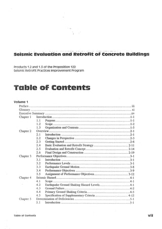
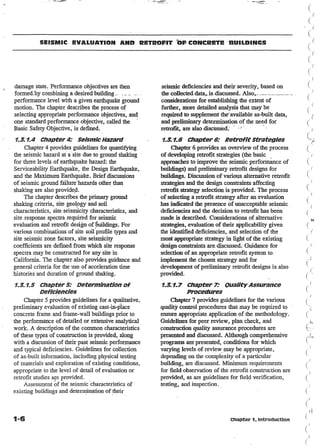
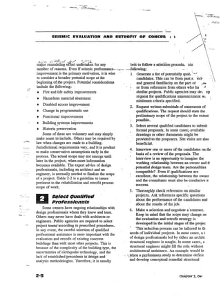
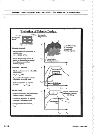
- Ground -Motion· & Response-Spectra
a
t
HIlHIHfl~IfIDt1M~,-.-
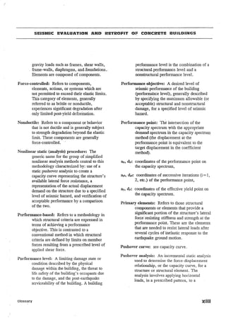
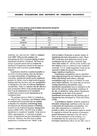
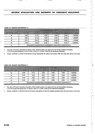
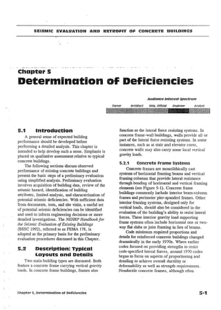
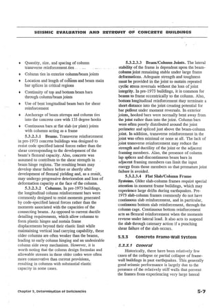
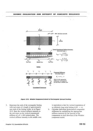
Ground motion recordings (accelerograms) indicate that ground
shaking is an extremely complex waveform, containing oscillatory
motion components over a broad range of frequencies.
-g~
]
.
By performing a time history analysis of a structure
~
it is possible to determine the peak acceleration, .-<:
velocity and displacement of the structure's response to
a ground motion. If such analyses are performed for
a series of single degree of freedom structures, each having a
different period, T, and the peak response accelerations. velocities ~
and displacements are plotted vs. the period of the structures, the _
resulting graphs are termed respectively acceleration, velocity and
displacement response spectra.
~
T
tee
T
~L
..!!
~
T
Period
Researchers commonly display response spectra on a 3axis plot known as a tri-partite plot in which peak response
acceleration, velocity and displacement are all plotted
.
simultaneously against structnral period. Researchers
(Newmark and Hall, 1982) have found that response spectra for'
typical records can be enveloped by a plot with three distinct
ranges: a constant peak spectral acceleration (PSA), constant
peak spectral velocity (PSV) and constant peak spectral
displacement (PSD).
PSA
Response spectra contained in the building code
indicate the constant acceleration and velocity ranges
... plotted in an acceleration vs period domain. This is
convenient to the code design procedure which is
based on forces (or strength) which are proportional
., to acceleration.
21'C(PSV)/I'
.§
E
~
]
Period - T
21'C(PSV)/I'
T2
Chapter 4, Seismic Hazard
For nonlinear analysis, both force and deformation
are important. Therefore, spectra are plotted in an
acceleration vs, displacement domain, which has been
termed ADRS (acceleration-displacement response spectra)
(Mahaneyet al.,1993). Period in these ADRS are
represented by a series of radial lines extending
from the origin of the plot. See also Converting
to ADRS Spectra in Chapter 8.

76. (-~
~(
(
(
SEISMIC EVALUATION AND RETROFIT OF CONCRETE BUILDINGS
(
"
(
(
4.4.5.2 Site-speciFic Hazard Analysis'·
..- Studies. . ... .. .. --'---'-
(
....-..- .. -.-.r-:-=-,.,..".--=,........,....."",...."..,.---.,..,....."....,.,..,.....",,----~
..
Site-specific hazard analysis studies should be
performed for buildings situated on site soil profile .
type SF, and are recommended for buildings on site .
soil profile type.SE. Site-specific studies should also
be performed for certain buildings situated near .
active sources and for buildings with special design
requirements (e.g., hospitals, base-isolated
buildings). In all cases, the assumptions and
methods used in the site-specific studies should be
consistent with:·the definition of the earthquake
hazard level(s) of interest given in Section 4.2.
The site specific studies should develop
estimates of short- and long-period response for
each hazard level of interest. The value of CA
should be taken to be equal to 0.4 times the spectral
response acceleration (units of g) at a period of 0.3
seconds. The value of Cv should be taken to be
equal to the greater of either 1.0 times the spectral
response acceleration (in units of g) at a period of
1.0 seconds or 1/Tefftimes the spectral response
acceleration (in units of g) at the effective period
Teff of the building. The effective period Teris based
on the secant stiffness at the point of maximum
response, as described in Chapter 7.
For each hazard level of interest, the values of
CA and Cv should not be taken as less than 80 .
percent, and need not be taken to be greater than
100 percent, of the values specified in Table 4-7
and Table 4-8, respectively.
.
4.4.~.~
Construction of an Elastic
Response spectrum
An elastic response spectrum, for each
earthquake hazard level of interest at a site, is based
on the site seismic coefficients CA 'and Cv, defined
in the previous sections. The seismic coefficient CA
represents the effective peak acceleration (EPA) of
the ground. A factor of about 2.5 times CA
represents the average value of peak response of a 5
percent-damped short-period system in the
acceleration domain. The seismic coefficient Cv
represents 5 percent-damped response of a l-second
system and when divided by period defines
Control Periods
1 2 •SCA I
·..
·
i
Ts = Cyl2.5C A
TA
=D.2Ts
(
(
(
(
t I~PA=CAI
~.
,
..
(
,
,.
·
·
i
(
Period (Seconds)
(
Figure 4-'1. construction of a 5 percent-Damped
Elastic Response spectrum
acceleration response in the velocity domain.
Figure 4-1 illustrates the construction of an elastic
response spectrum.
(
(
I"!!
('"
(
4.5~
Specification of
supplementarv" Criteria
4.5.1
Acceleration Time Histories
(
(
t,
When required for analysis, not less than three
pairs of horizontal time history components should
be selected from earthquake groundmotion records.
A set of sev~n or more pairs of time history
components is recommended and would be
necessary for the design to be based on the average
(rather than the maximum) value ofrhe response
quantity of interest.
Recorded earthquakes should be selected to
have a magnitude, source characteristics, and
distance from source to site that is the same as (or
consistent with) the magnitude, source
characteristics and source-to-site distance of the
event that dominates the ground shaking hazard at
the building site. Recorded earthquakes should also
be selected to have site conditions that are the same
as (or consistent with) the site conditions of the
building. When three appropri~te recorded ground
(
(
(
(
(
(
(
,
4-12
Chapter 4, Seismic
Hazard
~
(
(

77. Table 4·9. Earthquake Records at Soil Sites crester Than 10 Km From Sources
1
7.1
1949
western washington
station 325
USGS1
2
6.5
1954
Eureka, California
station 022
USGS
3
6.6
1971
san Fernando, California
station 241
USGS
4
6.6
san Fernando, California
station 458
USGS
5
Lorna Prieta, California
Hollister, south & Pine
CDMG2
6
7.1
7.1
1971
,1989
1989
Lorna Prieta, California
Gilroy #2
CDMG
7
7.5
1992
Landers, california
Yermo
CDMG
8
l.
1992
Landers, california
Joshua Tree
CDMG
6.7
1994
Northridge, California
Moorpark
CDMG
10
2,
7.5
9
6.7
1994
Northridge, California
century City LACC NQJ1h
CDMG
USGS: United State Geological Survey
CDMG: California Division of Mines and Geology
motion time history pairs are not available,
appropriate simulated ground motion time history
pairs may be used to make up the total number
required.
The intent of these requirements is that each
pair of time history components have an appropriate duration, contain near-source pulses (for
sites within 10 Ian of active faults) and include
other time domain characteristics that represent the
ground shaking expected at the building site.
Each pair of horizontal ground motion
components should be scaled in 'the time domain
such that the average value of the spectra of all
scaled time history components matches the site
response spectrum over the period range of
interest. The period range 'of interest includes, but
is not limited to, periods at or near the effective
period of the building associated with the
performance point determined by the nonlinear
static analysis procedure (Chapter 8). If highermode effects are being considered, then the period
range of interest should also include periods at or
near each higher-mode period of interest.
Commentary: A ground motion expert should
assist the structural engineer in the selection and
scaling of appropriate time histories.
Chapter 4, seismic Hazard
4.5.1.2 Earthquake Ground Motion
Records
Two sets of ,10 earthquake records each have
been identifiedas suitable candidates for time
history analysis. One .set contains records at sites
at least 10.kin from fault rupture and the other set
contains records at sites near fault rupture (e.g.,
sites within about 5 kID of fault rupture). Tables
4-9 and 4-10 list these earthquake records,
respectively. and summarize key attributes.
All ground motion records listed in Tables 4-9
and 4-10 meet the following criteria:
+ Free-field station (or ground floor of a small
building)
,
+ Stiff or medium soil site conditions
•
Large-magnitude earthquake (M;::: 6.5)
+ Peak ground acceleration of at least O.2g
(before scaling)
These records, after appropriate scaling, are
suitable for time history analysis of buildings at all
sites (except soft or very soft soil sites) for ground
shaking of 0.2 or greater EPA.

78. (=
(
(
(
((
:
c
(
Table 4·10. Earthquake Records at soil sites Near Sources
--1
6.5
1979
Imperial valley, california
EI centro Array station 6
USGS'!
2
6.5
1979
Imperial valley, California
EI centro Array station 7
USGS
3
7.1
1989
Lorna prieta, california
corralitos
COMG2
4
7.1
1989
Lorna prieta, California
capitola
COMG
5
1992
Cape Mendocino, canrornla
Petrolia
COMG
6
6.9
6.7
1994
Northridge, california
NeWhall Fire Station
COMG
7
6.7
1994
Northridge, California
svlmar Hospital
COMG
8
6.7
1994
Northridge, california
9
6.7
Northridge, California
SVlmar converter sta. East
6.7
Northridge, californi~
Rinaldi Treatment Plant
LAOWP
,-(
(
LAOWP
10
1994
"1994"
.-,
. sylmar Converter station
LAOWp3
(
(
(
(
(
(
(
l.
2.
3.
USGS: United States Geological Survey
CDMG: California Division of Mines and Geology
LADWP: Los Angeles Department of Water and Power
(
(1:
Figure 4-2 is a plot of 40 percent-damped
response spectra of the two horizontal components
of each of the 10 earthquake time histories listed in
Table 4-9 and the mean and mean + 1 standard
deviation of these 20 spectra. A dampinglevel of
40 percent is used to represent the equivalent
viscous damping of a building that has yielded
significantly, as described in Chapter 8. Each of
the 10 pairs of horizontal components have been
scaled such that their 5 percent-damped response
spectra approximately match the response spectrum shown in Figure 4-1 for CA = 0.4 and,Cv =
0.6.
Figure 4-2 compares the response spectrum of
each' earthquake component and the mean (or
mean + 1 sigma) response spectrum of the
ensemble of all earthquake components.
Significant differences typically exist between
mean (or mean + 1 sigma) response and that of
individual components, even though each
component represents the same site and source
conditions and has been scaled to match a common
target spectrum. Figure 4-2 illustrates that
predictions of response (and performance) using
smooth design spectra can significantly
underpredict or overpredict response (and
perforinance) that the building actually experiences
during the design earthquake.
4.5.2
(
(
(
criteria for Duration of Ground
Shaking
.
... dO'.-... i
The duration .of ground shaking should be
considered when selecting time histories and when
determining an appropriate level of effective
damping for the structural system. Effective
damping is usedto determine the response level of
demand spectra, as described in Chapter 8.
Structural systems that degrade with repeated
cycles of high seismic demand will have reduced
energy absorption (damping) capacity. The amount
of degradation and the associated reduction in
effective damping increases 'with the number of
cycles at or near the peak demand level.
Two distinctly different earthquake scenarios
should be considered when evaluating duration
effects on potential structural degradation and
reduction in damping capacity. The first
(
(
(I.
(
(
(
(
"
(-
4·14
Chapter 4, seisinic Hazard
(
-.

79. :
~ 0.6
c
o
~
0.4
Cii
o
o
<:(
ro 0.2
...
ti
Q)
o,
en
0.0 +-----+-----+------1-----1
o
246
6
Spectral Displacement (Inches)
Figure 4-2. Response spectra (40% Damping) of the
Earthquake Records Listed in Table 4-9
earthquake scenario is important for sites near a
seismic source (fault). In this case, a relatively
short duration of very strong shaking would be
expected because of the proximity of the site to
fault rupture. The ground may shake for a
considerable period of time (depending on the
earthquake magnitude), but there would likely be
only a few cycles of very strong pulses at the level.
of response described by the site spectrum (i.e.,
large spectral demand over a relatively short
duration). For the purpose of determining an
appropriate level of effective damping
(Section 8.2.2), sites with a near-source factor, N
~ 1.2, may be assumed to have short-duration
ground shaking.
The second earthquake scenario is important
for sites far from fault rupture (far from the
causative source). In this case, a much longer
duration of ground shaking would be expected at
the level of response described by the site
Chapter 4, seismic Hazard
spectrum (i.e., small/moderate spectral demand
.over.a.relatively long duration) ... Although, ground ....
shaking is not as strong in the second scenario, a
longer duration of shaking increases the potential
for degradation of the structural system. For the
purpose of determining an appropriate level of
effective damping (Section 8.2.2), sites located In
seismic zone 3 should be assumed to have longduration ground shaking unless a properly
substantiated geotechnical study recommends
otherwise.
For sites located in seismic zone 4 (with a
near-source factor of N < 1.2), ground shaking
duration ( in terms of the number of cycles of
demand at or near the peak demand level described
by the site spectrum), will depend on the
magnitude of the earthquake and the site soil
profile (and possibly other factors). For the
purpose of determining an appropriate level of
effective damping (Section 8.2.2), sites located in
seismic zone 4 (with a near-source factor of N <
1.2) should be assumed to have long-period
ground shaking unless either the seismic source
that governs ground shaking hazard at the site has
a maximum moment magnitude of M::; 6.5 and the
site soil profile is rock or stiff soil (i.e., soil
profile type SB, Sc or SD), or a properly
substantiated geotechnical study recommends
otherwise.
Commentary: An important potential
contributor to duration could be long-period
resonance at soil sites due to basin effects. Long
duration ground shaking should be assumed for
soft soil sites unless a geotechnical study
recorrunends otherwise.

80. .(
(
{
(
-(
:
(
(
(
(
.(
(
(
i
(
(
(
(
(
(
t-
(
i
(
(
I
(
i
(
I
(

81. SEISMIC EVALUATION AND RETROFIT OF CONCRETE BUUDINGS
:
Chapter
s
Determination of Deficiencies
AUdience Interest spectrum
owner
5a'l
Introduction
A general sense of expected building
performance should be developed before
performing a detailed analysis. This chapter is
intended to help develop such a sense. Emphasis is
placed on qualitative assessment relative to typical
concrete buildings.
The following sections discuss observed
performance of existing concrete buildings and
present the basic steps of a preliminary evaluation
using simplified analysis. Preliminary evaluation
involves acquisition of building data, review of the
seismic hazard, identification of building
attributes, limited analysis, and characterization of
potential seismic deficiencies. With sufficient data
from documents, tests, and site visits, a useful set
of potential seismic deficiencies can be identified
and used to inform engineering decisions or more
detailed investigations. The NEHRP Handbookfor
the Seismic Evaluation of Existing Buildings
(ESSC 1992),referred to as FEMA 178 is
adopted as the primary basis for the preliminary
evaluation procedures discussed in this Chapter.
Sa2
Description: Typical
Layouts and Details
Two main building types are discussed. Both
feature a concrete frame carrying vertical gravity
loads. In concrete frame buildings, frames also
Chapter 5, Determination of Deficiencies·
Architect
Bldg. Official
function as the lateral force resisting systems. In
concrete frame-wall buildings, walls provide all or
part of the lateral force resisting systems. In some
instances, such as at stair and elevator cores ,
concrete walls may also carry some local vertical
gravity loads.
5.2.1
Concrete Frame Systems
Concrete frames are monolithically cast
systems of horizontal framing beams and vertical
framing columns that provide lateral resistance
through bending of horizontal and vertical framing
elements (see Figure 5-1). Concrete frame
buildings commonly include interior beam-column
frames and perimeter pier-spandrel frames. Other
interior framing systems, designed only for
vertical loads, should also be considered in the
evaluation of the building's ability to resist lateral
forces. These interior gravity load supporting
frame systems often include horizontal one or twoway flat slabs or joist framing in lieu of beams.
Code minimum required proportions and
details for reinforced concrete buildings changed
dramatically in the early 1970s. Where earlier
codes focused on providing strengths to resist
code-specified lateral forces, around 1970 codes
began to focus on aspects of proportioning and
detailing to achieve overall ductility or
deformability as well as strength requirements.
Nonductile concrete frames, although often

82. t(
(
(
-(
SEISMIC EVALUATION AND RETROFIT OF CONCREtE Bun.DiNGS
(
.i.
'1
C
;:
(
-(
It
rr-~~~~LJ-~~~~LJ-~~~~Ll-~~~~Ll-~~~~LJ-~~~-£l~~~~-£l~~~~-n
II
I I
II
/I
I !
/I
II
I I
II
"
.1 I...
/I
/I
I ..L
/I
II
II
II
"
II
II
II
II
II
II
II
II
"
"
/I
/I
I I
"
"
"
II
II
I I
"
"
"
"
II
I I
"
II
II
II
/I
I I
II
II
II
II
II
I I
II
II
II
II
"
II
II
II
/I
II
II
I I
II
II
II
II
II
I I
II
/I
II
"
II
"
II
II
II
II
II
II
II
II
II
II
II
II
/I
II
II
II
II
II
"
II
II
II
II
II
II
II
II
II
"
II
"
"
"
"
"
II
"
"
"
/I
"
"
"
"
"
II
"
II
II
II
II
II
II
II
II
II
II
II
II
II
II
II
"
II
II
II
II
II
II.
II
II
II
"
II
II
II
II
II
II
II
II
II
II
!.I
II
. ! J.__..
I'
(
II
...__... .
/I
_J.. l .... _.. __ L ~. __... __
H- - - - - H- - - - - H- - - - - H- - - - - H- - - - - H- - - - -H- - - - - -H- - - - - +4
,.,.- - - - - H- - - - - H- - - -- - H- - - - - H- - - .- - H- - - - -H- - - - - -H- - - - - +.J
(
.
(
(
(
(
[
(
f
(
D: : : : : 0: : : : : 8: : : : : [J: : : ==0: : : : : [J: : : : tt : : == : tt : : : : :tl
Figure 5-1. Typical Concrete Frame Layout
designed to resist lateral forces, did not
incorporate the special detailing provisions now
required for ductile concrete.
In pre-1970s concrete frame construction, it is
common to find inadequate lap splices for mai:D.
reinforcing bars and a lack of adequate transverse
reinforcing ties (see Figure 5-2). Lap splices in
columns generally occurred just above the floor
level where stress levels are highest. In addition,
the column lap splices were generally very short,
often only 30 bar diameters or less in length, and
were typically not confined with closely spaced
column ties. Main beam reinforcing was generally
designed for code force levels, not considering
effects of post-yield behavior. Beam topbars were
often terminated 6 to 8 feet from the coluiDn face.
Beam bottom bars were typically discontinued at
the face of the supporting column or provided. with
only a short lap centered on the column. The .
spacing of beam and column ties was typically
wide by today's standards. Column ties often
consisted of a single hoop with 90 degree hooks
spaced at 12" to 18" on center. Beam ties, often
sized only for gravity shear loads, were spaced
closely near the column face but widely spaced or
discontinued throughout the mid-span region of the
beam.
The affect of these typical conditions and
deficiencies on seismic performance is discussed
below.
i..
(
(
(
(
(
(
(
.1
(
(
(
Discontinuous
Reinforcement
1._--- Widely spaced
ties
!~---
(
Short lap
splice in high
stress region
(
(
(
(
Figure 5-2_ Typical pre-1970s Frame Elevation
(
(
Chapters, oetermination of Deficiencies
~'
(
(
(
(

83. ------y-----tr"------i--j j---- j----- -ii-j ---1 l ii - - - ~----:::tI
:..1- - - - -
I
I
I
I
I
I I
I I
I I
II
II
~::
I
I
I
I
I
I I
II
I I
I I
I I
I
I
I
I
II
II
I
I
-.-e-_-
IL-I.'·
...
------~-------
I
I
I
I
I
I I
I I
I
I
I
:: :::= := r - - - - - .. ::::= ~ :: ----mHo.~~+-: : :
I
I
I
I
I
I
I
I
I
~---------
II
II
I I
I I
II
I I
II
I I
II
II
I I
II
II
I I
I I
I I
I
II
II
llII-a - - - ~f-
---
-
I
I
I
I
I
I
I
I
I
I
:p:: : :: : :
II
II
I I
-~
'Hi,
II
II
I I
I I
II
II
I I
II
II
II
II
II
II
II
I I
I I
I I
II
I I
I I
I I
II
I I
I I
I I
II
I I
I I
I I
II
II
II
II
II
II
I I
I I
II
I I
I I
I I
JJ
l-l- - - - - u- - - - - w- - - - :;J;;l; - - - I I - - - - -U- - - - ----llIiii!lIIi.B---~----~---~---
r .
I' ,
l
)0----
Figure 5-5. Typical Concrete Frame-Wall Layout
5.2.2
Concrete Frame-Wall Systems
Concrete frame-wall buildings typically
possess a complete gravity frame system,
essentially independent of the concrete walls, to
support vertical loads (see Figure 5-3). However,
in some instances concrete walls may carry some
local vertical gravity loads.
Concrete frame-wall buildings can include, for
example, exterior perforated walls with short piers
and deep spandrels, interior concrete walls near
stair and elevator cores, or perimeter frames with
concrete infill walls. The buildings in this category
generally have monolithically cast-in-place
reinforced concrete horizontal floor and roof
systems. Various concrete floor and roof framing
systems used with this building type include flat
plate, pan joist or beam, one-way slab, and twoway slab or waffle slab systems. Concrete framewall buildings were popular for institutional uses,
such as government offices, hospital wards,
schools, university buildings, court buildings, and
prisons.
The layout of wall locations was, to a large
part, dictated by functional considerations. In
many older buildings it was the only consideration.
Chapter 5, Determination of Deficiencies
Floor plans that induce torsion, lack significant
torsional rigidity or have eccentric or skewed walls
often resulted. Perimeter walls typically contain
numerous window and door openings. In
multistory buildings, the openings were frequently
arranged in a regular grid. This pattern of
openings gives rise to the pier and spandrel system
composed of relatively deep spandrel beams and
relatively short and wide wall piers. Floor framing
systems were often not designed to function as
diaphragms, with collectors, drags and struts,
capable of distributing floor inertial loads to The
isolated interior andlor perimeter walls. Also,
adequate provisions to transfer the lateral load out
of the walls into the foundation system are often:
lacking.
In existing, pre-1970s construction, it is
common to find walls without confined boundary
elements (see Figure 5-4). Vertical reinforcement
lap splices were usually designed for compression
loads only, in which case they may' be inadequate
for the flexural tension that may develop under
realistic earthquake loads. Horizontal
reinforcement also may be inadequately anchored.

84. ---~.
(
(
SEISMIC EVALUATION AND RETROFIT OF CONCRETE BUILDINGS
(
('
(
-
-----~
Open
Boundaty
v: element
. --Without - - .__.--
.
confinement
V
Short lap
lengths
I
I
--1---------1"
'~'
~"
I
,'"
I
Minimal
reinfolCing
at openings
1
I
I
1
-T-----·---T-
,
----5
4
i-
~
,
1
<,
"
~
r
J
.. 100.
....._
No hooks fa. ~a.
cu
.choiaga
Figure 5·4. Typical ere-tsros Wall configuration
Wall thickness and transverse reinforcement
were often sized to resist code-specified lateral
forces rather than the shear corresponding to
development of the wall's flexural capacity, so
almost all walls in these older buildings are shear
critical. Often, adequate attention was not paid to
construction joints, resulting in there being
weakened planes in the vertical wall system.
Walls with openings have been designed and
detailed in a variety of ways, the choice depending
on the expected behavior of the wall. Analysis
methods used in design were commonly based on
the assumption that the openings did not interrupt
the monolithic form of the wall; interrupted
reinforcement is placed at the boundary of the
opening and diagonal steel may be placed across
the comers to control cracking.
Where openings are more substantial, current
V .S. practice is to calculate stresses at the
boundaries of the wall segments. lithe stress
exceeds O.2fe, confined boundary steel is placed.
_. _This. boundary..reinforcing_steelis_often.not presenL ..__
in older construction.
Where substantial wall openings are aligned
vertically, the connecting segments may be
designed as coupling beams. Ductile coupling
beams in buildings designed to meet current U. S.
codes are detailed with continuous top and bottom
(and possibly diagonal) reinforcement that is well
anchored into the wall. As required by some
current codes, deeper coupling beams may be
designed to have diagonal reinforcement. Coupling
beams in older construction often lack many of
these detailing characteristics,
Beam transverse reinforcement with closed
hoops having 135 degree hooks, provides shear
strength, confines the concrete, and restrains
longitudinal bar buckling. Shear reinforcement is
now proportioned to resist the shear corresponding
to development of beam flexural strengths.
In pre-1930s construction, it is common to
find concrete infill walls. The concrete infill was
typically on the order of 6 to 8 inches thick and
generally contained light reinforcement, such as
3/8-inch diameter bars at 24 inches on center, in a
single curtain near the center of the wall. In many
cases, the reinforcing of the infill did not continue
into the surrounding gravity frame, creating a
weakened plane around the infill boundaries.
Furthermore, the concrete used in the infill was
generally of lower quality than that used in the
surrounding gravity frames. The concrete frames
for these· buildings were designed exclusively as
gravity-load-supporting frames. As a result, these
frames do not have the lateral stiffness and
strength to resist code-level design lateral forces.
Furthermore, they generally lack the reinforcingcontinuous beam bottom bars through joints,
continuous top beam bars at midspans, and shear
reinforcement or ties throughout the full beam
span-necessary to resist even moderate lateral
forces.
The affects of these typical conditions on
seismic performance is discussed below.
(
,(
(
(
(
(
('
(
(
(
(~
(
(
(
(
(
(
'(
(
(
('
chapter 5, Determination of Deficiencies
t
(
(
I
I"

85. SEISMIC EVAl.UATION AND RETROFIT OF CONCRETE BUILDINGS
:
5.3
Seismic Performance
5.3.1
csneral
The seismic performance of a structure is
dependent upon the performance characteristics of
its critical components. The critical.components
are those that are necessary for vertical stability
and those that comprise the seismic load path. In
all buildings.' seismic inertial forces originate in
the components of the structure and are transferred
through connections to horizontal diaphragm
systems. The horizontal diaphragm systems
distribute these inertial forces to vertical lateral
force resisting elements which in tum transfer
these forces to the foundations. When connections
or elements along this seismic load path are'
subjected to forces and/or deformations that
produce unacceptable damage states, deficiencies
exist. When the elements of the structure that
provide vertical stability can no longer maintain
that capability, deficiencies exist.
Through observation of building performance
in past earthquakes, a number of general building
characteristics have been identified that have been
responsible for localized component deficiencies.
These characteristics include a discontinuous
seismic load path, lack of redundancy in the
vertical shear'resisting system, vertical
irregularities (abrupt changes in stiffness, strength,
or mass), plan configuration irregularities, and the
presence of adjacent structures which may
potentially interact under seismic excitation. Any
of these characteristics could occur in concrete
frame or concrete frame-wall buildings. Detailed
analytical procedures can be used to establish to
what extent these building characteristics cause
unacceptable building performance, However, .
recognizing that these factors exist in a building is
a key consideration in developing an understandingof the building's expected seismic performance.
Component and connection seismic
performance can be thought of in terms of
response characteristics that are either force
controlled or deformation controlled. Force
controlled behavior is characterized by essentially
Chapter 5, Determination of Deficiencies
elastic behavior that abruptly terminates in
material.rupture and subsequent.rapid.deterioration
or disintegration. Once a critical force is reached
in the element/connection, it experiences a rapid
drop in· stiffness and strength. This is frequently
described as brittle behavior. Deformation
controlled behavior is characterized by essentially
elastic performance until a critical force threshold
is attained beyond which deformation continues
with little or no increase, or decrease, in capacity.
At this plateau, the component can continue to
deform until material strain limits are exceeded at
which point rupture, crushing, fracture or slippage
occurs. At this limiting deformation, a sudden loss
of stiffness and/or strength may also occur. This is
frequently described as a ductile behavior pattern.
Unacceptable seismic performance in concrete
frame and frame-wall buildings, especially those
designed and constructed before the early 1970s, is
most often attributable to force controlled or brittle
failure mechanisms. General discussions of the
seismic performance of concrete systems and
individual members found in frame and frame-wall
buildings are available in several recent
publications such as Paulay and Priestly (1992)
and Ferguson et al. (1988).
5.3.2
Concrete Frame systems
5.5..2. 1 General
Concrete frame construction has several
potential failure modes that directly threaten the
structure's ability to' sustain vertical loads and
maintain stable lateral behavior. The largest
concern.is a brittle c~lumn failure mode caused by
shear failure or compression crushing (due to
combined axial, flexural, and P-L1 effects) of the
concrete. Systems that exhibit some (limited)
yielding modes can also eventually form dangerous
collapse mechanisms as a result of stiffness or
strength degradation at sections without ductile
detailing. Punching shear failure in two-way slab
systems, for example, can instigate local collapse
of the floor. Also, localized concentrations of drift
due to-soft or weak story configurations are of
serious concern. The challenge for the engineer is

86. (
(
SEISMIC EVALUATION AND RETROFIT OF CONCRETE BUILD_NGSt
(
(
(
to identify all possible ways a frame building can
fail, .determine.the..sequence, of failure..and.then. .
find ways to preclude catastrophic modes of
response to seismic ground motion.
5..3.2.2 Typical conFiguration
DeFiciencies
Configurational deficiencies commonly found
in concrete frame structural systems, such as an .
incomplete load path, vertical and/or horizontal
irregularities, and inappropriate columnlbeam
relative strengths can Iead to failure of individual
members and connections.
5.3.2.2.1 Incomplete Load Path. A
complete and continuous seismic load path is
essential for the proper seismic behavior of a
structure. Missing links in the load' path must be
identified. Load path evaluation should begin by
establishing the source of all lateral loads
generated throughout the building, and then
tracking how those forces travel through the
structurai systems; from the diaphragms to the
vertical lateral force resisting elements, through
various joints and connections, to the foundations.
5.3.2.2.2 Vertical Irregularities. Vertical
irregularities typically occur in a story which is
significantly weaker, more flexible or heavier (due
to a greater mass) than stories above or below.
These irregularities are normally due to significant
changes in building configuration such as setbacks,
discontinuous vertical elements, or changes in
story heights. However, they sometimes arise due
to more subtle and less easily observed changes to
column dimensions, size and number of main
reinforcing steel, or column tie spacing. Vertical
irregularities are difficult to appreciate by a visual
inspection or simplified estimation. FEMA 178
(ESSC 1992) provides quick checking procedures
for concrete frame story capacities and drifts that
can provide preliminary assessment for vertical
irregularities.
'
5.3.2.2.3 Horizontal Irregularities.
Horizontal irregularities of the concrete frame
buildings are typically due to odd plan shapes, re-
(
entrant comers, or diaphragm openings and
..
discontinuities..These.deficienciea.often cause-. ---- _ _.-_.
significant differences between the building's
centers of mass. and rigidity (in one or more
(
stories), resulting in the torsional response of the
building to seismic ground motions. Such torsional
irregularities lead to concentrated demands on
(
diaphragms and excessive deflections at building
ends. In many cases, conditions at adjacent stories
(
can affect the stiffness properties of the irregular
story.
(
5.3~2.2.4 Weak Column/Strong Beam.
Optimum seismic performance is gained when
(
frame members have shear strengths greater than
bending strengths and when bending strengths of
(
the columns are greater than the beams. These
features provide a controlled failure mode and, in
.multistory frames, increase the total energy
(
absorption capacity of the system. In older
concrete frame buildings, where the beams are
often stronger than the columns, column hinging
can lead to a story mechanism, creating latge. p(
delta effects and inelastic rotations in the columns.
Column hinging is undesirable since this may lead
to loss of the column's gravity load carrying
ability after only a very few cycles. Furthermore,
(
although isolated column hinging may be tolerable
(
in some circumstances, hinging of most or all of
the columns on a single level will result in the loss
(
of lateral stability. FEMA 178.provides local joint
analyses for frames to evaluate the potential for
these effects.
5.5.2.8 Detailing concerns
In general, most concrete frame buildings built
before 1973 will contain an array of nonductile
detailing of the reinforcing steel. As a result, these
nonductile frame buildings exhibit a wide range of
generally poor seismic performance, .especially
once the elastic deformation limits of the concrete
members are exceeded. Reinforcement detailing
conditions which should be investigated for
deficiencies in the preliminary evaluation include
the following:
o
I
(
(
(
(
(
"I;
(
Chapter 5, Determination of Deficie-ncies
(
(
~>'

87. SEISMU:: EVAL,UATION AND RETROFIT OF CONCRETE BUU.DINGS
:
•
Quantity, size, and spacing of column
__.
transverse reinforcement-ties
..
Column ties in exterior columnlbeam joints
+ Location and length of coliimn and beam main
bar splices in critical regions
•
Continuity of top and bottom beam bars
through colurnnlbeam joints
•
Use of bent longitudinal beam bars for shear
reinforcem~nt
•
Anchorage of-beam stirrups and column ties
into the concrete core with 135 degree hooks
•
Continuous bars at flat slab (or plate) joints
with columns acting as a frame
5.3.2.3.1 Beams. Transverse reinforcement
in pre-1973 concrete buildings was designed to
resist code specified lateral forces rather than the
shear corresponding to the development of the
beam's flexural capacity. Also, concrete was
assumed to contribute to the shear strength in
beam hinge regions. The resulting beam may
develop shear failure before or shortly after
development of flexural yielding and, as a result,
may undergo progressive deterioration and loss of
deformation capacity at the face of the column.
5.3.2.3.2 Columns. In pre-1973 buildings,
the longitudinal column reinforcement bars were
commonly designed to resist moments generated
by code-specified lateral forces rather than the
moments associated with the capacities of the
connecting beams. As opposed to current ductile
detailing requirements, which allow columns to
form plastic hinges and sustain frame
displacements beyond their elastic limit while
maintaining vertical load carrying capability, these
older columns are often weaker than the beams,
leading to early column hinging and an undesirable
column side sway mechanism. However, it is
worth noting that the column design formulas and
allowable stresses in these older codes were often
more conservative than current provisions,
resulting in columns with substantial elastic
capacity in some cases.
e,
Chapter 5, netermlnatton of Deficiencies
5.3.2.3.3 Beam/Column Joints. The lateral
. stability ofthe frame. is dependent.upon the.. beamcolumn joint remaining stable under large frame
deformations. Adequate strength and toughness
must be provided in the joint to sustain repeated
cyclic stress reversals without the loss of joint
integrity. In pre-1973 buildings, it is common for
beams to frame eccentrically to the column. Also,
bottom longitudinal reinforcement may terminate a
short distance into the joint creating potential for
bar pullout under moment reversals. In exterior
joints, hooked bars were normally bent away from
the joint rather than into the joint. Column bars
were often poorly distributed around the joint
perimeter and spliced just above the beam-column
joint. In addition, transverse reinforcement in the
joint was often minimal or none at all. The lack of
joint transverse reinforcement may reduce the
strength and ductility of the joint or the adjacent
framing members. Also, the presence of column
lap splices and discontinuous beam bars in
adjacent framing members can limit the input
energy from those members so that premature joint
failure is avoided.
5.3.2.3.4 Flat Slab/ColUmn Frame
Systems. Older slab-column frames require special
attention in moment frame buildings, which may
experience large drifts during earthquakes. Pre1973 slab-column frames commonly do not have
continuous slab reinforcement, and in particular,
continuous bottom slab reinforcement, through the
column cage. Continuous bottom reinforcement
acts as flexural reinforcement when the moments
reverse under lateral load. It also acts to suspend
the slab through catenary action if a punching
shear failure of the slab occurs.
5.3.3
Concrete Frame-Wall system
5.5..5.. 1 General
Historically, there have been relatively few
cases of the collapse or partial collapse of framewall buildings in past earthquakes. This generally
good seismic performance is largely due to the
presence of the relatively stiff walls that prevent
the frames from experiencing very large lateral

88. -~.
~~-
(
(
Vertical discontinuity
i
-- --(
Wall
infill
(
(
l;/
(.l
Foundation
1.-
Figure 5-5. Typical vertical DiscontinuitY
displacements and deformations. Also, the presence
of an essentially complete vertical load carrying
space frame eliminates the need for the walls to
retain their vertical load carrying resistance
throughout the seismic response. Where collapses
have occurred, they have been traced to irregular
wall layouts, insufficient connections along the
seismic load path, poor concrete quality, inadequatereinforcement anchorage, or a grossly inadequate
quantity or distribution of the walls.
The presence of these building attributes can
give rise to a range of specific building
component/connection failure mechanisms. These
mechanisms include vertical discontinuities, weak
stories, perforated walls, coupling beams, shear
cracking, diagonal tension/compression, sliding
shear, reinforcement anchorage and confinement
and foundation anchorage and uplift. The challenge
to the engineer is to identify the possible ways
frame-wall buildings can degrade, to determine the
sequence of failure, and to find ways to control the
degradation to preclude catastrophic modes of
response.
5.:5.:5.2 Typical DeFiciencies
5.3.3.2.1 Vertical Discontinuity. The
primary negative structural impact of a vertically
irregular placement of wall panels, in which an
upper level wall (particularly one at an interior
column line) is not continued directly down to its
foundation, is that the columns below the ends of
the discontinued wall are subjected to large,
concentrated overturning reactions (see Figure 5-5).
Frequently, these columns have been designed to
resist only gravity loads. Under extreme seismic
loading, the columns can experience forces well in
excess of their compressive capacity and suddenly
lose their ability to sustain gravity loads. These
columns may also experience net uplift tension
forces for which insufficient reinforcement has been
provided. These types of force controlled failures
can be sudden and catastrophic. They are
considered serious deficiencies when the seismic
force levels exceed the available column axial load
capacities. A secondary structural impact of this
type of deficiency is that the diaphragm at the level
of the discontinuity is required to transfer large
shear forces from the discontinued wall and
redistribute it to other available walls below. -Often,
the floor diaphragms are not designed for this
redistribution of wall shears and can become very
highly overloaded
5.3.3.2.2 Weak Stories. Irregular placement
of interior wall panels can result in significant
changes in strength and stiffness from floor t~
floor. Of particular concern is a reduction in the
number of shear wall panels at the ground floor
level. This abrupt strength and stiffness reduction
results in a floor level whose vertical shear resisting
elements are likely to reach their limit response
states before the walls in the floors above have
(
(
(
"
(
(
(
(
(
(
((
(
(
(
(
(
(
Chapter 5, Determination of Deficiencies
(
,
(

89. :
Coupling
.. beams
Shear
wall ..
Coupling Beam Actions
Foundation
Figure 5-6. Typical coupling Beam
reached the elastic limit of their response. As a
result, the weak or soft story will undergo large
lateral displacements in comparison to the floors
above. This concentration of lateral displacement
can lead to severe demands on the columns that
provide the structure's vertical stability. A weak
story is considered a deficiency if it can lead to a
loss of vertical stability at the seismic hazard level
associated with the target performance objectives.
5.3.3.2.3 Perforated Walls and
Pier/Spandrel Conditions. Perimeter walls
frequently feature a large number of openings for
windows and doors. These openings typically
occur on a repeated module that provide an
appealing symmetry. The perforated wall that
results, acts to resist seismic forces as a
wall/frame wherein the piers act as column
elements and the spandrels act as beams. In older
frame-wall buildings, the piers are often only
lightly reinforced, for both shear and flexure.
While concentrated amounts of vertical reinforcing
may be found at locations where a concrete
column occurs, most often the column occurs at
the middle of the wall piers and does not
appreciably contribute to the lateral capacities of
the wall pier. As a result, the piers are underreinforced for both the shear forces and the
concentrated flexural tensile and compressive
forces that result in the pier due to seismic actions.
The limited amount of tensile reinforcement can
result in relatively low flexural capacity of these
Chapter 5, Determination of Deficiencies
elements. The spandrel elements will perform in a
manner similar to frame beams. As noted for
coupling beams, these elements can be a
deficiency if they are not reinforced adequately for
theforces they develop in the piers. The behavior
of these elements will typically be deformation
controlled but can be a serious deficiency if.
yielding occurs at very low lateral force levels.
This is true for all performance levels.
5.3.3.2.4 Coupling Beams. Beam elements
that are attached to adjacent shear walls tend to
couple the seismic resistance of the walls as if they
were columns joined in a moment frame. If the
depth of the beam is sufficient, its stiffness may be
great enough to restrain the rotation of the walls
significantly. However, the spandrel beam must be·
strong enough to sustain the corresponding shear
forces and end moments associated with this
frame-like behavior and, in many older buildings,
there often is not sufficient reinforcement provided
to accomplish this. Differences in taller wall pier
stiffnesses due to axial tension and compression
forces can cause tension to occur in coupling
beams as the pier, in compression, resists more
load than the pier in tension. As a consequence,
shear wall coupling beams can exhibit rapid
diagonal tension failures (see Figure 5-6) similar
to that described in Section 5.3.3.2.5 below.
The failure of these elements can result in
spalling of the concrete at or near the joint to the

90. -
)
(
(
(
::
(
(
(
V· Seismic shear
~
Reinforcement
Rapidly opening
cracks can lead to
spalling of concrete and
reinforcement buckling
when seismic fOrc~
reverse direction
•
~....,..,.........",=,...,,~_.
Shear
-- ~--'----- wall
---,---Diagonal crackpattern
(
,
r,
Foundation
Figure 5·7. Typical Shear cracking pattern
wall sections. Since coupling beams are frequently
located either on the perimeter of the building or
over areas of the structure that serve as exit
corridors, the degradation of these elements can
create a falling hazard, which poses a minor to
moderate Hie safety ~rsk to passersby or persons
exiting .from the building.
Additionally, failure of these elements decouple the adjacent shear walls, thereby changing
their effective stiffness. Often, this can represent a
beneficial effect. Thus, coupling beam deficiencies
may be considered acceptable seismic performance
for both the Life Safety and "Structural Stability
performance objectives provided that any resulting
.
permanent offset of the structure is within
permissible bounds, stability Under gravity loads is
maintained, and falling debris does not jeopardize
life safety.
5.3.3.2.5 Shear Cracking .and Diagonal
Tension/Compression. Walls that resist
earthquake forces can exhibit diagonal patterns of
cracking that are attributable to the development of
stresses in the concrete that exceed the concrete's
principal tensile stress. The onset of shear cracking
is generally not considered a serious deficiency
unless there is an insufficient amount of
reinforcing steel in the wall to maintain
deformation controlled behavior.
Minor shear cracking is considered an
acceptable damage state for even the Immediate
Occupancy performance objective if ductile,
deformation controlled, behavior is maintained;
More extensive shear cracking is considered
acceptable for both the Life Safety and Structural
Stability performance objectives. in all instances,
shear cracking is an acceptable damage state for .
concrete shear walls provided that adequate
reinforcement is' provided to control the width of
the cracks. When the reinforcement is insufficient,
the widths of cracks open rapidly, which can lead
to buckling of the reinforcement and degradation
of the wall's ability to sustain vertical loads (see
Figure 5-7). A shear wall that is substantially
under-reinforced can thus exhibit brittle, force
controlled behavior and represent a serious
deficiency, once the force level associated with
initial cracking is reached, for higher levels of
desired performance.
Walls that are more heavily reinforced and are
subjected to extreme seismic demands may also
exhibit force controlled behavior related to shear
cracking. This can occur when compressive
stresses are developed that exceed the concrete's
compressive strength. When diagonal tension
cracks form, it is generally held that a series of
inclined tension and compression struts. act to resist
the shearing forces in the wall panel. When the
compression strut force exceeds the compressive
capacity of the concrete, crushing will occur (see
Figure 5-8). Such a failure mode, when subjected
to repeated reversing cycles of earthquake loading,
can lead to the generally gradual loss of the
(
(
(
(
I
(
(
(
(
I
(
Ii
5-10
Chapter 5, Determination o~ beficientles
C
(

91. :
__ .
..__ ..
._.'
.
...
..
.
V-Seismic shear
--..-
.. _ r - - - - - - , . , ;
Shear wall
. ". __.
...
...
.._.. _ . __
.. -.
Diagonal crack
pattern
Reinforcement
Compressive
strut
Foundation
Figure
Compressive
forces exceed
concrete capacity
and a crushing
. - ' - - - ' - 1 - - - - - - - ' - - - , failure occurs
s-e. Typical Combined Shear cracking /
wall's ability to sustain large gravity loads. A
deficiency of this type can occur When there is a
grossly inadequate amount of wall provided, weak
or disintegrated concrete is present, and the wall is
subjected to large gravity loads. Similar to
.
coupling beam failures, shear cracking/diagonal
tension failures can be considered acceptable if
permanent offsets are within permissible bounds
and stability under gravity loads is maintained.
5.3.3.2.6 Sliding Shear. Sliding shear
failure can occurat a weak plane, such asa
construction joint, or along flexural cracks that
have opened up or propagated, after several
cycles of loading, to form a shear failure plane. In
addition, formation of a shear failure plane can .
occur after concrete crushing has occurred at both
ends of a wall.
Once a crack has been established across the
section, shear forces are resisted only by the
doweling action of the reinforcing steel crossing
the crack or joint. Continued cycles of seismic
load reversal can cause kinking or fracturing of
this reinforcement. Once a significant number of
reinforcing bars have been bent or broken,
resistance to seismic shearing forces can only be
mobilized through frictional resistance along the
shear plane. This form of resistance is force
controlled and can lead to significant permanent
offsets which, if great enough, can result in
vertical instability. Sliding Shear failures can be
Chapter 5, Determination of Deficiencies
compression Failure
considered acceptable s~ismic performance for
both the Life Safety and Structural Stability
performance objectives provided that any resulting
permanent offset of the structure is within
permissible bounds and stability under gravity
loads is maintained.
.
5.3.3.2.7 Reinforcement Anchorage and
Confinement. The lengths of reinforcing bar lap
splicing used in older concrete buildings is often
not sufficient to develop the yield capacity of bars.
In shear walls, where flexural behavior is
important, insufficient lap lengths of the boundary
reinforcing can lead to bar slip before the
development of yield stresses in the reinforcing.
Inadequate confinement of the concrete at wall
boundaries can also limit the effectiveness of the
lap splices used for vertical boundary reinforcing
3.J."1.d of the anchorage of horizontal wall
reinforcing. Premature slippage of reinforcing is a
significant modeling concern that should be
accounted for by the use of a reduced reinforcing
capacity. Once reinforcing slippage begins to
occur, a brittle, force controlled mechanism can
result. In the case of vertical boundary
reinforcement, slippage can be accompanied by a
loss of flexural resistance which leads to a
progressive deterioration of the wall boundaries.
The slippage of horizontal wall reinforcement can
aggravate development of shear cracking in the
wall. The damages resulting from this type of
5-11

92. (
(
(
(
SEISMIC EVALUATION AND RETROFIT OF CONCRETE BUn.DINGS
(
(
(
:
(
deficiency may be considered to be acceptable
seismic...performance for.either the. Life Safety-or-_ ...
Structural Stability performance objectives
provided that any resulting permanent offset of the
structure is within permissible limits and stability
under gravity loads is maintained.
5.3.3.2.8 Foundation Anchorage and
Uplift. Analogous to the lap splice condition
described in Section 5.3.3.2.7 above, the length of
embedment used in older buildings for anchorage
of the vertical wall reinforcing into the foundations
is often not sufficient to develop the yield capacity
of the bars. The resulting slippage of the
reinforcement can lead to the same kind of
performance as described for inadequate lap
splices.
In older concrete buildings, the footings that
support concrete walls were sized for gravity
loads. The large
concentration of
force at the ends of
shear walls
resisting seismic
loads can exceed
both the tributary
dead load at the
foundation or the
compressive
bearing strength of
the soils. Such
conditions can give
rise to foundation rocking. The phenomena of
foundation rocking tends to reduce the effective .
stiffness of the wall. This can have a variety of
effects, either beneficial or detrimental, on the
building's seismic performance. Rocking could
lengthen the building period sufficiently to actually
reduce the force demand, thus actually protecting
force critical elements in some cases. Rocking
could, however, also lead to significantly larger
displacements than would be predicted by fixed
base modeling and thus contribute to potential
vertical load carrying instabilities due to the P - L1
effect. A detailed discussion of foundation effects
on seismic performance is provided in Chapter 10.
5-112
The potential for foundation flexibility or rocking
.should be.assessed.during..the..preliminary----. -_... - . . ..
evaluation of deficiencies.
5.4
Data Collection
5.4.1
Introduction
The seismic evaluation of existing concrete
buildings depends on data collection as a factual
basis. The data collection process includes
acquisition of available documents, field
observations, field investigations, materials
testing, and documentation. While the extent of the
data acquisition process will vary from building to
building and will depend on the availability of
drawings and the level of evaluation being
performed, i.e. preliminary evaluation, detailed
evaluation and analysis, or preparation of final
retrofit construction documents, accurate
building information is
necessary, in any event,
<.in the following areas:
. • Building geometry,
configuration, and
mass (including
structural,
architectural and
mechanical systems)
• Elements of the
seismic load path,
including frames, walls, diaphragms,
foundations, and connections
+ Configuration and layout of structural
members, including size of members, size of
reinforcing, tie spacing, splice locations, and
concrete cover
• Properties of the materials used in the
structural system, such as concrete and steel
reinforcing
• Anchorage of nonstructural elements
Tables 5-1 through 5-4 summarize the data
collection process as it relates to availability of
drawings and level of evaluation. The tables
Chapter 5, Determination of Deficiencies
(
l~
(
(
(
(
(
(
(
(
(
(
(
(
I
(

93. provide guidance for the applicability of the
specific data.collection,items.for.which the__ ...
following sections provide more detailed
descriptions.
Commentary: The amount of information
gathered should be sufficient to perform the
various levels of evaluation and analysis discussed .
in this document, yet it may be imprudent to collect more information than necessary for a specific
stage in the evaluation process. For example, if it
is not clear whether retrofitwill be required; the
data collection process should be geared towards
gathering just enough information to make that
determination, whereas once the determination to
retrofit has been made, the data collection process
will usually be much more extensive.
It may not be necessary to identify the
configuration and layout of all structural members
in the building. However, as required by the level
of evaluation, information should be acquired for
all structural members that either are part of the
seismic load path (e.g. walls and diaphragms) or
are necessary for vertical stability of the structure
and may be susceptible to failure because of
building accelerations or displacements during
earthquakes.
Acquisition of Available
Documents
The single most important step in the data
collection process is the acquisition of documents
describing the existing construction. The review of
construction drawings will simplify field work and
lead to a more complete understanding of the
building, especially considering that no amount of
field investigation and testing can substitute for the
information available in the original drawings.
Acquisition of the original architectural and
structural construction drawings is often critical to
an accurate and cost effective evaluation. Potential
resources include the current building owner,
building departments, and the original architects
/engineers. In some cases, drawings may also be
available from architects or engineers who have
performed prior evaluations for the specific
building. If drawings cannot be located, substantial
.....effort,will be.required.to, document.the..existing - .
construction, even for preliminary evaluation of
deficiencies, and a detailed evaluation of the
structure will require extensive field testing.
In addition to construction drawings, it may be
helpful to acquire, to the extent possible, the
following documents:
.. Structural calculations
..
Site seismicity I geotechnical reports
..
Foundation reports
..
Prior building assessments
5.4.3
Field Observations
It is of paramount importance that the
evaluating engineer conduct field observations of
the building. Though the extent will vary
depending on the evaluation requirements, primary
purposes and types of the field observations typical
for most projects are as follows:
• Verification of the accuracy of the original
drawings or determination of basic building
information if no drawings are available
..
Identification of major alterations not shown
on the original construction documents. Major
additions and alterations are not uncommon
and may have significant impacts on the
'*
seismic performance of the building
..
Identification of visible structural damage,
such as concrete cracking or spalling.
Structural damage or cyclic degradation caused
by prior earthquakes, deterioration, or poor
quality original construction may reduce the
available structural capacity of the building
..
Identification of potential nonstructural falling
hazards, including ceilings, partitions, curtain
walls, veneer, mechanical systems, fixtures,
and other nonstructural building elements
..
Documentation of existing conditions with
photographs at key locations. These
photographs often serve as a useful verification
tool during the evaluation process
5.4.2
Chapter 5, Determination of. Deficiencies .

94. :
(
Table 5-1. inFormation Ilequir"ed For preliminary seismic Evaluation When original .
._co..nstructi~/!-,~~a.rJ!!!1!fls..~/:.eA.v.aj!F!P.!..f!!.
.__ _.
_.
.
(
.
._.
.
(
(
structural calculations
x
Helpful but not essential
Site selsmtcltv, geotechnical
report
x
Helpful but updated report should be none
Foundation report
x
Helpful but not essential
prior seismic assessment reports
x
(
Helpful but not essential
Condition survey of building
Alteration and as built assessment
x
x
Nonstructural wall< through .
(
(
(
.X
walk through dimensioning
(
x
unless required by undocumented alterations
(
Identify falling hazards, weight.
Core testing
x
Unless concrete appears substandard
Rebound hammer testing
.x
Unless concrete appears substandard
Aggregate testing
x
Reinforcement testing
x
Reinf. location verification
x
Nonstructural exploration
x
unless insufficient info. on drawings
Table 5-2. Information Ilequired For prMiminary seismic Evaluation When original
Construction Drawings are Not Available
(
(
(

95. :
Table 5-5. Information eequired For a Detailed seismic Evaluation When Original
.
.._ . __.__ ....
.
constructfqn.p..r?.wiJ1g?-~rfE...-9.Yf!fJ?!lj!l..
__
prior seismic assessmentreports
x
..
._ ---
Helpful.but not essential
x
.
could be very helpful
Foundation report
x
x
x
----.-.--
spot checking is appropriate
structural calculations
site seismicity, geotech rpt,
Condition survey of building
.'
Arteratton and as built assessment
Helpful but not essential
Helpful but not essential
x
x
l!I!alkthrough dtmenstonlns
Nonstructural wi:3lk through _
Identify falling hazards, weight
core testing
x
Minimum 2 per floor, 8 per building
Rebound hammer testing
x
x
Minimum 8 per floor, 16 per building
Aggregate testing
Each core
x
Reinforcement testing
optional
Reinforcement location verification
x
pachometer @ 10% of critical locations, visual
locations
Nonstructural exploration
x
verify anchorage and bracing conditions for
components sensitive to Building performa'nce
@
2
Table 5-4. Information eequired For a Detailed Seismic Evaluation When original
construction Drawings are-Not Available
.
.x
x
x
x
structural calculations
site seismicity, geotech rpt,
Foundation report
prior seismic assessmentreports
could be very helPful
Helpful but not essential
Helpful but not essential
Helpful but not essential
Condition survey of building
x
Alteration and as built assessment
Walk through dimensioning
x
x
Nonstructural walK through
x
Identify falling hazards, weight
x
x
x
x
x
Minimum 8 per floor, 16 per building
Each core
2 per type-
core testing
Rebound hammer testing
Aggregate testing
Reinforcement testing
Reinforcement location verification
Nonstructural exploration
Chapter 5, Determination of Def!ciendes
Must be done very thoroughly, particularly if structure
will be retrofitted
Minimum 2 per floor, 8 per building
Pachometer for all critical elements, visual on 25%
Verify anchorage and bracing conditions for
components sensitive to Building performan'ce

96. (
(
(
SEISMIC EVALUATION' 4MD RETROFIT 'OF CONCRETE aUILDINGS
(
(
(
5.4.4
Materials Testing .
pachometer or exploration) in order to avoid
.Q<;Jrnaging..the_existing-stlUCtural-s-ystem..- ---'-----.. -. ---If-ori.ginal-constructiQn-doGuments-·are-a-vailable---: Commentary: The in situ concrete compressive
and no deterioration has been observed during the
strength is typically higher than specified on the
field observations, a preliminary evaluation may be .
construction documents. The testing, therefore, will
completed by using 'materials strength 'data from the
typically benefit the evaluation process by
documents.' However, the techniques for detailed
demonstrating the actual capacity of the existing
evaluations and analyses require accurate material
building materials. In some situations, however,
properties for evaluating the strength and stiffness
testing may identify low concrete strengths
of the building systems; elements, and connections.
attributable to poor quality of the original
If original construction data regarding the strengths.
construction or to deterioration due to adverse
of the materials are not available, a materials testing
environmental conditions.
program should be established to determine the in .
situ strength of the concrete and reiiiforcing steel
5.4.4.2 Rebound Hammer Testing
that serve as the primary structuralmaterials. Even
S41ce the number of core samples that can be
when the specified material strength data are
taken is limited because of the destructive nature of
available, a testing program should be undertaken to
sampling, rebound hammer testing should be
establish and/or verify the actual materials strength
performed to supplement the concrete strength data.
data for detailed analytical studies; .
A minimum of eight rebound hammer tests should
A typical detailed testing program should
be taken at each floor level, with a minimum of 16
include pachometer (resistance meter) testing to
test locations per building. Calibration of the
verify the existence and spacing of reinforcing bars,
rebound hammer testing should occur adjacent to
concrete core testing; "rebound hammer testing of
core test locations.
concrete, unit weight testing, of concrete aggregate,
and testing of steel reinforcement. Also, the
5.4.4..3 Aggregate Testing
concrete cover should be removed in a limited
.. The unit weight of the concrete should be tested
number of locations to verify the accuracy of the
to:determine whether lightweight aggregates were
pachometer readings and the bar sizes. The
used in the concrete construction. This information
evaluating engineer should determine the types and
can generally be obtained from the core samples
extent of testing based on the requirements of each
used for compression testing.
specific project.
.
5.4.4..4 ReinFOrcement Testing
5.4.4.1 Core Testing
Reinforcing samples should be taken from the
.Core testing provides a reliable method for the
building to determine the strength and deformability
determination of concrete compressive strength to
of the steel. Minimum test data should include
be used in the evaluation and analysis process. Core
stress' and straininformation at Yield and at rupture.
samples should be taken from critical structural
When required by the analysis procedures, a
elements such as shear walls, frames, and
minimum of two samples should be tested from
diaphragms. Because of the destructive nature of
each type of reinforcement (e.g., beam longitudinal
the coring process, however, testing can generally
steel, beam "ties, column longitudinal steel, column
be limited to two concrete"core samples for each
ties, slab reinforcing, wall reinforcing). In addition,
floor level, with a minimuin of eight samples per
if potential retrofit schemes include the welding of
building. However, if testing results vary widely,
existingreinforcing, chemical analysis of the steel
additional core samples may be required. Prior to
samples should be performed. to determine
coring, the existing ste~l should be located (e.g. by
equivalent carbon content.
!
(
(
(
(
(
.
(
(
5-16
Chapter 5, Determination of Deficiencies

97. :
5.4.5
Detailed Field Investigation
. . ... If adequate coastruotion decume1.lts--are----.--- - .. .....
available, detailed field investigation is not
necessary for a preliminary evaluation, Welldeveloped construction drawings, as confirmed by
field observations, are generally adequate to
identify the seismic load path, identify reinforcing
configurations, calculate the weight/mass of
building systems, and
identify the anchorage of
nonstructural elements.
If construction
documents for the building
are not available, detailed
field investigations will be
necessary to collect the .
building data described
above. Field investigations
for the collection of
building data can be a
daunting task, especially in reinforced concrete
structures. The field investigation program must be
tailored to each specific project, striking a balance
between obtaining the necessary data and keeping
the cost of the investigation program reasonable. In
many cases the structural elements are covered with
architectural finishes, and some removal and/or soft
demolition may be required in order to obtain the
necessary information. Furthermore; it will not be
possible to perform a detailed investigation on each
element of the structural system. Sound engineering
judgment will be required to conservatively
extrapolate results from a representative sample of
detailed inspections to the global building system.
Detailed building survey data should be .recorded in
a set of drawings that depict the buildings primary,
vertical and lateral force resisting system.
To perform detailed analyticalevaluations, it is
necessary that a materials testing program, similar .
to the one described above, be used, whether
drawings are available or not. To predict seismic
performance using the analytical procedures in this
document, it is necessary that concrete and
reinforcing strengths be well defined.
Determination of the onset of force controlled and
Chapter 5, oeterminatiqn .o.f Deficiencies.
deformation controlled component behavior cannot
be.made. in a.reliable.manner.without.this.L, .-- ..... ....
information.
Several techniques are useful in determining the
as-built reinforcement configuration in existing
buildings. In general, nondestructive testing such as
pachometer or X-ray testing Can be used to
determine the location and quantity of the
reinforcement. Exploratory probes
should be made in localized areas to
remove concrete cover and expose the
reinforcement and confirm the results
of the nondestructive testing.
As information is collected, record
drawings should be developed for the
building to document the gathered
information and identify areas where
additional information/investigation is
required. As a minimum, record
drawings should include structural
plan layouts of each floor level, details of
reinforcing conditions, identification of materials
strengths, and typical details used to brace
nonstructural elements. The documentation should
contain sufficient information to make it possible to
evaluate the strength and deforrnability of the
.
building systems.
5 ..5
Review
Hazard
of Seismic
Site characterization and seismic hazard
derivation are discussed in Chapter 4. There, 5
percent damped elastic response spectra for various
hazard levels are defined in terms of coefficients CA
and Cv. These coefficients may also be used with
FEMA 178 base shear equations for preliminary
analyses described in Sections 5.6 and 5.7.
The potential for ground failure should be
reviewed as described in Section 4.3. When ground
failure is deemed likely, the preliminary evaluation
described in Sections 5.6 and 5.7 is not sufficient.
Commentary: The simplified analysis methods
used for preliminary evaluation are not considered
adequate to account for ground failure or complex
soil-structure effects. "When ground failure is

98. (
(
(
SEISMIC EVALUATION AND RtsTRDFIT OF CONCRETl'!f BUII.DINGS
((
(
indicated, a geotechnical engineer should
recommend-mitigation. measures-or- pro.vide---.-" "parameters for a detailed analysis.
5 ..6
Identification of
Potential Deficiencies
5.6.1
Introduction
Potential deficiencies are conditions that might
lead to unacceptable performance at a local or . global level. Identification of potential deficiencies
requires only quick and limited analyses based on
available building information. These conservative
simplified analyses' are intended to find potential' ,
deficiencies that require detailed evaluation.
Commentary: A list ofpotential deficiencies
will generally serve as the basis for more detailed
analyses (Chapters 8-11) used to check acceptability
of the existing or retrofitted building, In some
..
instances it may be possible to identify deficiencies
of such a serious nature that the decision to retrofit
or abandon the structure can be made without
further study. This may be particularly true for
Performance Objectives r:equiring Immediate
Occupancy.
.
The engineer should understand the limited
precision of simplified analyses and should.define
potential deficiencies accordingly, Deficiencies
identified in this manner may not represent
conditions hazardous enough to jeopardize
structural stability or life safety. In most cases,
more detailed investigations are required to check
acceptability at the desired performance levels, .
hence the label "potential."
.
5.6.2
Definition of Seismic load Path
To identify potential seismic deficiencies, the
first step is to define the components (including
connections) that constitute the seismic load path. A
complete and adequate seismic load path is
fundamental to acceptable" seismic performance. All
existing buildings have a lateral load path of some
kind. Non-engineered structures and older buildings
not designed for lateral load resistance may have a
lateral load path that relies partly on friction or on
(
extremely weak or brittle components. When
.components-on-the...seismie-Ioad.path-are.. subjected~- - .
to forces or deformations that produce unacceptable
damage, deficiencies exist.
To define the seismic load path, first locate the
principal mass elements. In concrete buildings,
floor and roof diaphragms usually account for most
of the mass, and the lateral load resisting system
.it;seIf accounts for much of the rest. Next, identify
shear-resisting elements in each story that "link the
"masses to each other, typically walls and frame
c~l~. Determine,~:the method(s) of connecting
vertical shear resisting elements to horizontal
diaphragms.
5.6.3"
seteetlon of Evaluation
Statements
The recommended procedure for' identifying :
potential seismic deficiencies is based on "the
TruelFalse "evaluation statement" methodology ~f
FEMA 178-(BSSC 1992). After aseismic load path
for the structure has been defined, the most
appropriate set of FEMA 17.8 evaluation: statements
is selected.
Commentary: For most concrete buildings, only
three sets of evaluation statements will be needed:
General Evaluation Statements for foundations 'and
nonstruetural elements, Building Type 8 statements
for Concrete Moment Frames, and Building Type 9
statementsfor Concrete Shear Walls.
For purposes ofpreliminary. evaluation, FEMA
178 evaluation statements q.re most useful as
indicators of qualitative deficiencies. Their
systematic use by experienced engineers can be
expected to find deficiencies associated with
irregular building configurations, incomplete or
poorly-conceived structural systems, and some
inadequate- details. They should not be expected to
identify specific "local deficiencies without further
analysis. Refer t? Section5.6.4.3 commentary.
(
(
(
(
(
(
(
(
(
(
E
(
(
(
(
.
(
.;.
(
5-18
Chapter 5, DeterminatiOn of Deficiencies

99. 5.6.4
_
Simplified Analysis
_. ._.
_._.._.._ _.
._.-. _.-- ----------.-.. -----~- ---. --.
5.6.4.1 General
A simplified analysis provides relative
quantitative data for the preliminary evaluation
discussed further in.Section 5.7. Simplified analysis
results can also yield
insights useful for
modeling elements and
components for
detailed analysis
(Chapter 9).
Commentary:
Because simplified
analyses with linear
elastic properties do
not account for
inelastic deformations,
degrading strength, or force redistributions,
.
component forces are best understood ·in relative .
terms. For example, where inelasticity is.
anticipated, simplified analysis results can indicate
which components have the highest demands or are
likely to hinge first, but can not reliably predict
absolute stresses or plastic rotations. In general,
the analysis procedures ofFEMA 178 are
acceptable-. Refer to Section 5.6.4.3 commentary.
5.6.4.2 Mass
Seismic forces are proportional to the inertial
mass of the structure. The simplified analysis
requires mass estimates at each level of the
structure, considering both structural and
architectural elements. The estimate should include
ceilings, roof coverings, floor toppings, wall
covering, and other items considered permanent
parts of the building.
Commentary: In general, simplified analysis for
identifying potential deficiencies requires relative
forces only" However, if a detailed analysis per
Chapters 8 through 11 is anticipated, the use of
dead load plus likely live load (see Section 9.2) for
this simplified analysis can avoid some duplication
of effort. Also, useful demand/capacity ratios for
columns and other components subject to axial-
Chapter 5, Determination of Deficiencies
flexural load may require reasonably accurate
-.estimates.of- gm.vity..load.---,-_-- -- ---- -.- -- .
5.6.4.3 Global Demand
Because the preliminary evaluation is intended
to identify broad patterns of expected behavior,
useful results can be
obtained with any set of
lateral forces that
approximates. the
building's modal
response. A building
code or FEMA 178
force level and
distribution is simple,
convenient, and
sufficiently accurate. (If
FEMA 178 demands are
used, CA and. Cv values
from Chapter 4 may be used.) It is important to
keep in mind, however, that codes and handbook
documents like FEMA 178 often reflect particular
performance objectives that may be different from
those chosen for the subject building (see Chapter
3). Thus, while simplified analysis with these
demands may yield useful results, actual expected
demands (Chapters 3 and 4) may be quite different.
Commentary: FEMA 178 demands and
response coefficients (R values) imply a
Performance Objective ofLife Safety in a modified
Design Earthquake. If the subject building's
performance objective involves a different
earthquake or a different desired performance level,
FEMA 178 acceptance criteria might not be
appropriate. For preliminary evaluation, however,
the goal is a general understanding of expected
response, so absolute demand levels and
quantitative acceptance criteria are unimportant.
5.6.4.4 Component Demand
The seismic demand forces derived in
accordance with Section 5.6.4.3 must be distributed
to the various components (including connections)
that constitute the seismic load path. The
distribution may be made on the basis of relative

100. SEISMIC EVALUATION· AND RETROFIT OF CONCRETE BUILDINGS
;
(
,
".
(
~
rigidities of horizontal diaphragms and vertical
in contrast to the "detailed" approaches described in
(
shear. resisting elements.. Particular.artention.should.; _. ..Chapters B_thrOllg1Lll_The.prelimina ry_ ev:a1uation-- _.._..(
is intended to help develop a general sense of the
I"
be paid to portions of the load path where vertical
elements are discontinuous.
structure's expected performance in the absence of
(
Commentary: Approximate force distributions
a detailed analysis. The preliminary evaluation is
and hand calculations are appropriate for and
based on potential deficiencies determined in
(
consistent with the precision of this simplified "
acpordan.c~ with Section 5.6.
( -.
analysis. Labor intensive'
Commentary:~,
refinements will not
.Potential deficiencies
(
appreciably improve the
include high
demand/capacity ratios
('
precision ofthe'FEMA 178 ':
methodology.
.
and False evaluation
statements. As noted in(
5.6.4.5 Deficiency
Section 5.6.43, the global
Definition
demand usedfor simplified
(
To identify potential
analysis may or ma:y not
deficiencies, the force
(
'..approximate the seismic
actions are compared to
'. forces derived in
corresponding capacities 3$ .
accordance with Chapter 4
demand/capacity ratios
for the building's .
(DCRs). Demands for DCR'calculations must
performance objective. If they do, then rough'
include gravity effects. Evaluation statement
thresholds for acceptable DCRs ma:y be set based on
responses should be reviewed and completed in
engineering judgment and project-specific
light of calculated DCRs: High'Df'Rs and
requirements. If they do not, then absolute DCR .
conditions that yield 'False statements indicate
values must be read with. careful consideration of'
I
potential deficiencies.
(
differences between applied and expected demands.
Commentary: Capacities for DCR calculations
In general, the location and distribution of the
J
may be established with the FEMA 178 guidelines
critical. highest DCRs is most instructive.
and other reference sources that provide an estimate
The most critical potential deficiencies are those
( ,
of usable strength. "High DCRs" must be judged
which, if realized in an earthquake, can alter the
'.
considering the demands and capacities used arid
building's overall inelastic response. The
(
the building's actual performance objective.
consequences of potential inelastic response should
.
Assuming FEMA 178 demands and capacities, and
be considered at both local and global levels, as
,
a performance objective consistent w~th that
discussed in the following sections.
I
assumed 1:Jy FEMA 178; DCRs approaching 1.0 (or
(r
5.7.1
Member Inelasticity
higher) indicate potential deficiencies, whose
I
significance must be evaluated 1:Jy the engineer
(
For the highest demand/capacity ratio at each
(refer to Section 5.6.4.3 commentary).
floor and at each part of the load path (the locally
highest DCR), determine whether the associated
preliminary EVfJlluation
behavior is force-controlled or deformation5.7
(
controlled (refer to Figure 5-9 in Section 5.7.2, and
of Anticipated. Seismic
Section 9.5.4.1). Force-controlled actions more
Performance
(
frequently produce unacceptable seismic
The analyses and assessment methods described
( ,
perforinance. The highest force-controlled DCR
in this chapter constitute a "preliminary evaluation"
should be determined. Review the list of typical
I.
r
C
C'
(
-':'
5-20
(
Chapter 5, Determination of Deficiencies'
,
(
(

101. :
_________.
Deformationcontrolled
, ..
behavior
--,.
DCR demands must include gravity ejJeets.
._...,.
~Force­
controlled
behavior
Deformation
Figure 5-9: comparison of rorce-ws. Deformation.controlled Behavior
deficiencies (Sections' 5.3.2.2 and 5.3.3.2) for
Concrete Frame and Concrete Frame-Wall .
buildings and identify corresponding DCRs.
Locally highest DCRs in force-controlled
actions such as shear are critical deficiencies, and
locally highest DCRs in deformation-controlled
components may be critical deficiencies. Very high
DCRs in deformation-controlled components are
likely to reflect deficiencies since early yielding of.
these elements will concentrate inelastic
deformations among just a few members as opposed
to a more desirable distribution among many
members.
5.7.2
Respons~
Scenario
Global inelastic response can be understood as
the sequential yielding and degrading of individual
load path components. The sequence of yielding can
be approximated by listing demand/capacity ratios
from highest to lowest: Combined with
considerations of horizontal and vertical DCR
distributions, such a list suggests a "response
scenario," i.e. a conceptual representation of the
structure's anticipated seismic performance.
Commentary: Because forces in a real structure
are redistributed after some components hinge or
degrade, this approximation of hinging sequence is
only reasonable for the first few hinges, and only if
their DCRs are relatively close in value.
Chapter 5, Determination of De.ficiencies
If
... _...t_ e.propottum.ot.capacuy.usedfcar.gtasity, 1oad.--._._
he.uroootti
if.
.
.
•
id.eIy among cruica1 components, the .
..
vanes wz
sequence of hinging may be better approximated by
DEICE ratios as recommended by FEMA 178. 112 this
ratio, the demand is due to seismic loads only, and
the capacity is reduced to that available for seismic
loads after gravity loads have been applied.
The horizontal distribution of the highest
demand/capacity ratios should be noted. High
DCRs concentrated 'at'one end or in one portion of
the structure, indicate a potential for local failure or
loss of torsional stability. High ratios that are
scattered suggest that the onset of post elastic
structural behavior will be well distributed, a
beneficial attribute.
The vertical distribution and magnitude of the
highest demand/capacity ratios should be noted.
High ratios in vertical shear-resisting elements
concentrated at a particular level indicate a potential
weak story. As previouslynoted, such a deficiency
is common to Concrete Frame-Wall buildings.
5.8
preliminary Evaluation
Conclusions and
Recommendations
5.8.1
General
Preliminary evaluation findings should be
reported in a context that facilitates appropriate
decision making. In general, the preliminary
evaluation will support one of three basic options
(although others are certainly conceivable):
Retrofitting Recommended, Detailed Evaluation
Recommended, Performance Acceptable.
5.8.2
Retrofitting Recommended
When the preliminary evaluation reveals a
significant number of critical force-controlled
deficiencies, then a more detailed analysis may not
be needed to conclude that retrofit is required.
Conditions that may lead to this conclusion include
critical DCRs in force-controlled load path elements
without backup systems, locally highest DCRs
clustered at one floor (suggesting a weak story), and

102. (
(
SEISMIC EVALuaTION AND RETROFIT OF' CONCRETE BUILDINGS
(
(
:
<
(
(
. (
critical deficiencies at the perimeter of the building
(suggestingtorsional.instability). .Even.when..__._.__._. __ .. __
preliminary evaluation suggests strongly that retrofit
is required, detailed evaluation (Chapters 8-11) is
still expected to provide a more thorough ,.
understanding of expected performance.
5.8.3
Detailed Evaluation
Recommended -
For structures whose critical elements and
components are deformation-controlled, detailed
evaluation (Chapters 8 through 11) is usually
appropriate. Unless the critical demand/capacity
ratios are clustered or are extremely high, .
deformation-controlled deficiencies may not be so
severe so as to prevent acceptable performance. A
detailed evaluation may demonstrate acceptable
performance in structures that appear from
simplified analysis to be deficient.
5.8.4
Acceptable Performance
Only in very rare circumstances can acceptable
performance be reliably assured without detailed
analysis. As such, no general criteria for reaching'
this conclusion are available, although it is clear
that acceptable performance.based on preliminary
evaluation would certainly require very low
demand/capacity ratios (considering the actual
Performance Objective), "True" responses to all or
most evaluation statements, and reliable building
response scenarios.
5.8.5
affect the expected performance, then retrofit
. modifications.to.mitigate.its.effects-should be--.--....
recommended even if the' building is otherwise
acceptable. This is .true for potential ground failures
as well.
(
(
(
5.8.5.2 Potential Nonstructural
DeFiciencies
Identification of nonstructural deficiencies is
presented in Chapter 12. Preliminary evaluation
conclusions should consider thenature and extent of
nonstructural deficiencies.
Normally, life safety concerns associated with.
nonstructural components are of greatest concern
(see Table 5-5). Besides the potential risk of
components falling directly on building occupants,
some components (e.g. hazardous materials,
pressurized piping) pose secondary hazards. Life
safety also depends on the ease of egress from an
affected building under emergency conditions. Both
high accelerations and' large relative displacements
can damage nonstructural·components. Chapter 12
provides further guidance on- the acceptability of
nonstructural damage depending on-the overall
performance goals for the building.
'
Commentary: If the scope of nonstructural
deficiencies is extensive, retrofitting may be the
most cost effective approach. If architectural
finishes must be removed in large areas in order to
mitigate nonstructural deficiencies, a significant
portion of the cost of modifying' an underlying
structural component will already be incurred.
(
(
(
(
(
(J
f
(
(
(
other considerations
.-
.
5.8.5.1 Related structural Hazards
Adjacent structures that may interact seismically
with the subject building should be considered in
the preliminary evaluation conclusions and
recommendations: If pounding appears likely to'
5.8.5.. :5 Additional Testing
When preliminary evaluation conclusions rely
on assumptions or incomplete information,
additional testing may be warranted before a course,
of action is determined. Additional testing. can also
be used to rule out potential deficiencies.
(
(
(
(
5-22
Chapter 5, Determi~~tion of Deficie~cies
(
(
(

103. Table 5-5. cenerst Characteristics of Nonstructural component (adapted From ATc;. 1996al
./
./
./
./
./
./
prefabricated panels
./
./
./
Glazing systems
Partitions
Adhered veneer
Glass blocks
Exterior skin
./
./
./
Heavy
./
./
./
./
./
Light
Ceilings
stone, including marble
./
./
./
Ceramic tile
Interior veneers
./
./
./
./
Directly applied to
structure
Dropped, furred gyp.bd
./
suspended lath &
plaster
./
./
-:
./
suspended jntegrated
Parapets and appendages
./
./
canopies and marquees
./
./
Chimneys and stacks
./
./
stairs
./
./
./
./
Equipment
Boilers and furnaces
Mfg. and process mach.
HVAC eouio.usoiatern
HVAcequip.
tnonlsolatern
storage vessels
./
./
./
structural supported
./
./
Flat bottomed
High pressure piping
./
./
./
Fire suppression piping
./
./
./
./
./
./
./
./
./
./
Fluid piping
Hazardous materials
Non-hazardous
DuctworK
Chapter 5, Determination o~ Defi~ienCi.es

104. (
('
(
(
(
SEISMIC EVALUATION AND' RETROi='IT OF CONCRETEr SUU.DINGS
:
(
(
-1'
-T-able-s-S.-fContinuedJ-oeneraJ.characreristiG5-of-NonstrUGrupal-Gomponent-fsdapted-Fpom-A-TG;-- -_. ----.- .--(
199Ga)
(
(
(
(
(
Light fixtures
C
t
Recessed
Surface mounted
Integrated ceiling
(.
pendant
(
(
(
storage racks
.1
Bookcases
(
computer floors
(
Hazardous materials storage
(
cornputer/comrn. racks
(
Elevators
("
conveyors
('
(
('
(
('
(
('
(
('
(
(
Chapter 5 Determination of Deficiencies
ti
(
I
(
(
(

105. :
.........
_-_._ ..-
-.~'-_
Chapter
..
--_.._._.__
6
_._-_._---_._ ..__.- - _..-. _. -- _
_.
etrofit strategies
AUdience Interest spectrum
Owner
6 .. 'I
Intrcduct·ion
6.1.1
General
This chapter presents an overview of the
process used to develop a retrofit strategy and
preliminary retrofit design for a building once an
evaluation has been conducted in accordance with
Chapter 5 and the presence of unacceptable seismic
deficiencies has been detected. It includes
discussion of alternative retrofit strategies,
evaluation of their applicability given the identified
seismic deficiencies and the various design
constraints, selection of the most appropriate
strategy in light of these constraints, and within the
context of the selected strategy, selection of an
appropriate retrofit system and development of a
preliminary retrofit design.
For most buildings and performance
objectives, a number of alternative strategies and
systems may result in acceptable design solutions.
Prior to adopting a particular strategy, the engineer
should evaluate a number of alternatives for
feasibility and applicability and, together with the
owner, should select the strategy or combination of
strategies that appears to provide the most
favorable overall solution. It is not possible to do
this until the owner's performance objectives for
the building have been identified and an evaluation
of the building has been performed. This
evaluation will determine whether the building is
Chapter 6, Retrofit strategies
Architect·
Bldg. Official
capable, in its existing configuration, of providing
this performance and, if not, the extent of the any
existing deficiencies.
Commentary: Traditionally, engineers
performing seismic evaluations and retrofit designs
have used a code-based approach. The process
was initiated by evaluating the adequacy of the
building to resist lateral forces with a specified
"base shear, " typically taken to be in the range of
75 percent to 100 percent of the base shear
.
specified by the building code for design of new
structures. Typical deficiencies identified in such
an evaluation would be that certain elements of the
building's lateral force resisting system were
'significantly "overstressed" or that lateral drifts
were excessive. Based on these findings, engineers
would then design new supplemental lateral force
resisting elements, such as shear walls or braced
frames, in order to eliminate the calculated
overstress conditions and reduce lateral drifts to
acceptable levels. In some extreme cases,
engineers would design the new elements to
provide the entire lateral force resistance for the
structure, negating their need, if not the building's, to rely on the existing element's behavior.
This traditional approach is both
straight-forward and simple to apply. However, it
frequently leads to design solutions that are less
than optimal given considerations of cost, effect on
building appearance, and other pertinent factors.
Further, in many cases this traditional approach

106. -
.... ~.
(
(
will not lead to a technically acceptable design
strength and stiffness to the lateral force resisting
solutioiu.lhe. building code provisions.for. new. . --_._. __ ._-system.- detailed.evaluation: of-man:y- alter.p.ativ.e..~-_ ...- construction have closely related requirements for
strategies is neither warranted nor necessary.
I
both lateral strength and detailing. It is typically
Nevertheless, forlarge structures or for;,builtf,ings
(
., 1'ff.th 'complex structural systems, the additional
impossible to upgrade an existing building to
I
(
conform with the detailing requirements of the
effort involved in the evaluation of alternative
retrofit strategies, as suggested in this chapter, can
current building codes. Upgrades that address only
the code strength requirements without also
result in significant reductions in retrofit cost and
addressing the detailing requirements can not be
lead to design solutions that are more appropriate
expected to provide the same performance as that
than those that would otherwise be obtained.
intended for new buildings.
, Prior to embarldng on a program that includes
Finally, there is the issue ofperformance itself.
consideration of many design alternatives, the
The performance objectives inherent in the building
engineer should exercise his or her individual
code provisions for new construction are based on
judgment to determine whether such effort is
(
consensus judgment as to an appropriate balance
warranted, given the configuration; deficiencies,
(
between initial construction costs, occupant safety
and performance objectives intended for the
(
and life time costs. This same balance may not be
building.
(
appropriate for many existing buildings, suggesting
Following selection of the retrofit strategy, it
(
that other performance objectives should be
is necessary to select a specific retrofit system and
selected as a basis for design. Unfortunately, the
perform a preliminary design. The retrofit system
and preliminary designare selected within the .
building code provisions do not currently provide a
means to design for alternative performance
context of the selected strategy. Generally, the
objectives.
same factors considered in the strategy selection .
The purpose of this chapter is to provide the
must also be kept in mind during system selection
engineer with a systematic approach for evaluating
and preliminary design.
(
the various strategies and systems that may be
Once a preliminary design is obtained,
verification of the adequacy of this design 'must be
applicable to a seismic upgrade project andfor
selecting the strategy and system that provide an
performed in accordance with the procedures of.·
(
optimal design solution, given the desired
Chapter 8 and using the acceptance criteria of
(
performance objectives, building characteristics
Chapter 11. If the preliminary design is- found to
and technical features of the existing structure. In
be inadequate, then it must be modified and the
(
addition to the traditional retrofit approaches
process repeated. When the verification analysis
described above, this chapter also includes
indicates that acceptable performance tan be
consideration of a number of strategies that are
obtained, final detailing of the design may be
more technically complex.
performed.
(
The methodology indicated for the evaluation
6.1.2
Definitions
(
of these various strategies to determine their
applicability is also somewhat complex compared
6.1.2.1 RetroFit strategies
with traditional code-based approaches of
.
A retrofit strategy is a basic approach adopted
structural evaluation. Often, the effort involved in
(
to improve the probable seismic performance of
evaluating multiple upgrade strategies and
the building or otherwise reduce the existing risk
selecting an optimal one can by itself be quite time
to an acceptable "level. Both technical strategies
consuming and costly. For simple structures, with
and management strategies can be employed to
deficiencies that can be simply and economically
obtain seismic risk reduction. Technical strategies
mitigated with the introduction of additional
l-
(
Chapter 6, Retrofit strategies
/
(
(
(

107. --
a. Unstrengthened building
b. Building with retofit braced frame
c. Building with retofit infill windows
Figure 5-1. Building with Perimeter concrete Walls
include such approaches as increasing building
strength, correcting critical deficiencies, alteringstiffness, and reducing demand. Management
strategies include such approaches as change of
occupancy, incremental improvement, and phased
construction.
Commentary: Engineers sometimes confuse
systems and strategies. Strategies relate to
modification or control of the basic parameters
that affect a building's earthquake performance.
These include the building's stiffness, strength,
deformation capacity, and ability to dissipate
energy, as well as the strength and character of
ground motion transmitted to the building and the
occupant and contents exposure within the
building. Seismic risk reduction strategies include
such approaches as increasing strength, increasing.
stif.fness, increasing deformability, increasing
damping, reducing occupancy exposure, and
modifying the character of the ground motion
transmitted to the building. Strategies can also
include combinations of these approaches. Retrofit
systems are specific methods used to implement the
strategy such as, for example, the addition of
shear walls or bracedframes to increase stiffness
and strength, the use of confinement jackets to
enhance deformability.
6.1.2.2 Retrofit system
A retrofit system is the specific method used to
achieve the selected strategy. For example, if the
basic strategy is to increase building strength, then
alternative systems that may be used to accomplish
Chapter 6, Retrofit strategies
this strategy could include addition of new shear
walls, thickening of existing shear walls, and
addition of braced frames. While the retrofit
systems are closely tied to the strategies, it is not
necessary to select a specific system in order to
evaluate the applicability of a given strategy.
However, it is necessary to select a specific system
in order to complete a design.
Commentary: One of the most important
considerations in the selection and design of a
retrofit system is its deflection compatibility with
the existing structure. Some existing buildings are
both weak and brittle, while also being quite stiff.
A common strategy for upgrading such a building
is to provide supplemental lateral strength. If such
strengthening is to be effective, the supplemental
elements provided to add this strength must be
sufficiently stiff that the added strength can be
mobilized prior to the onset of unacceptable
. damage to the existing elements.
As an illustrative example, consider the
concrete shear wall building illustrated in
Figure 6-1a. This building's seismic behavior is
controlled by the wall piers, present between the
windows. These wall piers have low shear strength
and could experience brittle shear failure if the
building experiences strong ground motion.
Although relatively weak, these piers are also quite
stiff. For the purpose of this example, it is
presumed that it has been decided to adopt a
strategy of structural strengthening.

108. (
(
((
(
(
Structural strengthening can be achieved by a
_.number...oJ-alterniztiY~stems,..two...otwhich..aT.cc...e
shown in the figure. Figure 6-1b illustrates a
system consisting of the addition of supplemental
braced steel frames. Figure 6-1c shows a system
consisting ofreinforced concrete infills within
existing window spaces. The braced frame system.
may be incompatible with the existing building.
That is, although the bracedframe could add
substantial strength to the building, it may not.be
practical to make this frame as rigid as the .
existing wall piers, which would therefore still
experience shear failure before the bracedframe
became effective. The window infills, shown in"
Figure 6-1c, however, having stiffness in excess of
that of the original building piers, would be able
to adequately protect the building against such
damage.
The methodology presented in this document
has been specifically developed to ensure appropriate consideration of the deflection compatibility
of retrofit systems with the existing structure.
6.1.2.:5 Design constraints
Design constraints are factors other than the
building's structural characteristics that affect the
ability of a retrofit strategy or system to be
effectively implemented. Design constraints that
may affect the applicability of a given retrofit
strategy include the intended performance
objectives, design and construction cost limits, the
project schedule, historic preservation .
requirements, the effects on building appearance
and floor space layout, the effects on building
occupancy both during and after project
construction, and issues of project risk.
Commentary: Design constraints are
typically set by persons other than the design team.
These can include political figures, who determine
the prioritization and scope of programs affecting
state-owned buildings': the client agency, which
determines project cost and schedule constraints;
the building occupants, who determine the functions that must occur in the building, the extent to
which the building will be occupied during
construction, the systems thatmust remain
oper.able..du:ting...aruLafter:...construction,..the_exteut.--- ..
to which floor layouts and visual effects may
change. and. the types of earthquake damage that
may be acceptable; the building official, .andfire
.marshal, who determine the extent to which.
collateral (i.e., disabled access andfire/life safety)
upgrades must be performed; historic preservation
boards, which determine the permissible extent of
alteration to historic fabrics and spaces; and
various special interest groups within the
community, which may have a significant ability to
affect the way in which a project is executed or
even prevent its execution.
6 ..2
(
-c('(
(
.
I
C
(
(
Alternative Retrofit
strategies
A wide range of technical and management
strategies are available for reducing the seismic
risk inherent in an existing building. Technical
strategies are approaches to modifying the basic
demand and response parameters of the building
for the Design'Earthquake. These strategies
include system completion, system strengthening,
system stiffening, enhancing deformation capacity,
enhancing energy dissipation capacity, and
reducing building demand.
Commentary: In the past, many engineers
have adopted a strategy of retrofitting the building
to "meet current code" or to provide a specified
fraction 'of the base shear capacity contained in the
current code. This is not really a strategy at all,
but rather a design criterion, often inappropriate,'
fOT use with one of the aforementioned strategies.
Basic approaches such as strengthening a
building, or stiffening it, or adding energy
dissipation capacity, aTe all strategies. Design
criteria pertain to the amount of strength," stiffness,
energy dissipation capacity, or other attributes
that are required in order to meet given
performance objectives. In this methodology, the
basic design criterion is to maintain damage to
critical elements of the building within levels
appropriate to the designperformance objective by
(
C
(
(
(
('
(
(
I
(
(
(
(
(
(:j
(
Chapter 6, Retrofit strategies
(
(
(

109. :
controlling lateral drift. Chapters 9 and 10 provide
... .design criteria that may be-used.respeciiveiy: in ..
judging the acceptability of likely damage to
structural and nonstructural components and
elements of the building under the Design
Earthquake. In general, these are not directly tied
to the building code.
In addition to technical strategies, a number of
alternative management strategies should also be
considered. Management strategies could include
decisions to implement the retrofit while the
building remained occupied; to vacate the building
until the retrofit could be performed; to accept the
existing risk and not retrofit; to change building
occupancy so that the risk is acceptable; to
demolish the building and replace it with an
alternative facility; to implement the technical
strategy on a phased basis over a number of years;
or to retrofit on a temporary basis until
replacement facilities can be obtained. Additional
management strategies could include performing
all work on the building exterior. possibly to
minimize the impact on building occupants, and
performing all work on the building interior, in
order to preserve the building's exterior
appearance.
Commentary: Management strategies have
often been regarded as beyond the design
engineer's scope of concern. Nevertheless, it is
ve7Y important that the engineer consider these
alternative management strategies and assist the
client in selecting an appropriate strategy. The
management strategy selected can have a great
effect on the feasibility and cost of implementing
the various technical strategies. Further, the best
solution for a building is often one that involves
management rather than technical action, such as
changing the building occupancy or constructing a
replacement facility.
Technical strategies
As a building responds to earthquake ground
motion, it experiences lateral displacements and,
in turn, deformations of its individual elements. At
low levels of response, the element deformations
6.2.1
Chapter 6, Retrofit strategies
will be within their elastic (linear) range and no
. damage.will.occur..At higher levels. of response,
element deformations will exceed their linear
elastic capacities and the building will experience
damage. In order to provide reliable seismic
performance, a building must have a complete
lateral force resisting system, capable of limiting
earthquake-induced lateral displacements to levels
at which the damage sustained by the building's
elements will be within acceptable levels for the
intended performance objective. The basic factors
that affect the lateral force resisting system's
ability to do this include the building's mass,
stiffness, damping, and configuration; the
deformation capacity of its elements; and the
strength and character of the ground motion it
must resist.
Commentary: The technical strategies
described in this methodology provide for
improved seismic performance by directly
operating on these basic response factors, either
individually or in concert. The traditional
approaches to seismic retrofit - the addition of
bracedframes and shear walls - operate on
building stiffness and strength. Energy dissipation
systems operate on the structure's damping
capability. Base isolation operates on the
character and strength of ground motion
transmitted to the structure.
There are a number of analysis procedures
(see Chapter 8) that compare measures of seismic
capacity and seismic demand to evaluate existing
structures. These methods are also useful to
investigate or verify the effectiveness of technical
retrofit strategies. The following discussion uses
the Capacity Spectrum Method to illustrate the
basic process.
The capacity spectrum is derived from an
approximate nonlinear, incremental static analysis
for the structure. In the process of performing this
incremental nonlinear static analysis, a capacity
curve is developed for the building. This capacity
curve is simply a plot of the total lateral seismic
shear demand, "V," on the structure, at various

110. (
(
SEISMIC EVA'LUAiION AND RETROFIT OF CONCRETE" 'BUIl.DINGS
(
;
v
,.,.,.
,.,.
,.,.
ai
e
0
,.' Effective stiffness
at displacement. Q
,.,.
, ,.
u..
t-
al
m
.r:
1. .- - Immediate Occupancy
.>:
level
, ,.'
en
e
S!
ttl
,,
...J
"iii
(
.;
ute
Safety level
,
,.,.
CollapseBll!>'
;§
,
Unear
elastic
range
Damage
Control
"'...;L.-J~
~:Pyr("-
(
/
I,'
d!,
D
(
" Lateral Displacement at'Roof
(
Increasing earthquake demand - -.......
(
Figu~e
6-2. TypIcal capacity curve
increments of loading, against the lateral deflection
of the building at the roof level, under that applied
lateral force. If a building had infinite linear elastic
capacity, this capacity curve would be' a straight
line with a slope equal to the global stiffness of the
structure. Since 'real buildings do riot have infinite
linear elastic capacities, the capacity curve
typically consists of a series of straight-line
segments with decreasing slope, representing the
progressive degradation in structural "stiffness that
occurs as the building is subjected to increased
lateral displacement, yielding, and damage. The
slope of a straight line drawn from the origin of the
plot for this curve to a point on the curve at any
lateral displacement, "d," represents the secant or
"effective" stiffness of the structure when pushed
laterally to that displacement A typical capacity
curve is shown in Figure 6-2.
In Figure 6-2, the discrete points indicated by
the symbol ... represent the occurrence of
important events in the lateral response history of
the structure. Such an event may be the initiation of
yield in a particular structural element or a
'it.
particular type of damage, such as spalling of cover
concrete on a column or shear failure of a spandrel
element. Each point is determined by a different
analysis sequence described in Section 8.2.1. Then,
by evaluating the cumulative effects"of &image
sustained at each of the individual events, arid the
overall behavior of the structure at increasing
lateral displacements, it is possible to determine
and indicate on the capacity curve"those total
structural lateral displacements that represent limits
on the various structural performance levels, as has
been done in Figure 6-2. Chapter 11 provides
specific guidance on"acceptance criteria that may be
used to determine the "lateral deformations for a
specific structure that correspond to these
performance limits based on story drift as well as
element and component strength and deformation
capacities.
Commentary: The process of defining lateral
deformation points on the capacity curve at which
specific structural performance levels may be said
to have "occurred requires the exercise of considerable judgment on the part of the engineer. For
.
.
Chapter 6. Retrofit strategies
;
I
C
1
(
(
(
(
(
(
(
(
/3:

111. SEISMIC EVALUATION AND RETROFIT OF CONCRETE
~UIILDING$
.:
each of the several structural performance levels
defined in Chapter 3,._ Chapterl lof this methodology defines global system response limits as well
as acceptance criteria for the individual structural
elements that make up typical buildings. These
acceptance criteria generally consist of limiting
values of element deformation parameters, such as
the plastic chord rotation of a beam or shear angle
of a wall. These limiting values have been selected
as reasonable approximate estimates of the average
deformations at which certain types of element
behavior such as cracking, yielding, spalling, or
crushing, may be expected to occur. As the
incremental static nonlinear analyses are
performed, the engineer must monitor the
cumulative deformations of all important structural
elements and evaluate them against the acceptance
criteria contained in Chapter 11.
The point on the capacity curve at which the
first element exceeds the permissible deformation
parameter for a structural performance level does
not necessarily represent the point at which the
structure as a whole reaches that structural performance level. Most structures contain many
elements and have considerable redundancy. Consequently, the onset of unacceptable damage to a
small percentage of these elements may not represent an unacceptable condition with regard to the
overall performance of the building. When determining the points along the capacity curve for a
structure at which the various structural performance levels may be said to be reached, the engineer must view the performance of the building as a
whole and consider the importance of damage
predicted for the various elements on the overall
behavior of the building.
This methodology incorporates the concept of
"primary" and "secondary" elements to assist the
engineer in making these judgments. Primary elements are those that are required as part of the
lateral force resisting system for the structure. All
other elements are designated as secondary elements. For a given performance level, secondary
elements are generally permitted to sustain more
damage than primary elemen.ts since degradation of
Chapter 6, Retrofit strategies
.
secondary elements does not have a significant
effect.on.the lateral load.resisting.capability of the.
building. If in the development of the capacity
curve it is determined that a few elements fail to
meet the acceptance criteria for a given
performance level at an increment of lateral
loading and displacement, the engineer has the
ability to designate these "nonconforming"
elements as secondary, enabling the use ofmore
liberal acceptance criteria for these few elements.
Care must be exercised not to designate an
excessive number of elements that are effective in
resisting lateral forces as secondary. Chapter 9
provides further guidance on this issue.
The capacity spectrum curve for the structure is
obtained by transforming the capacity curve from
lateral force (V) vs. lateral displacement (d)
coordinates to spectral acceleration (Sa) vs. spectral displacement (Sd) coordinates using the modal
shape vectors, participation factors and modal
masses obtained from a modal analysis of the
structure (see "Conversion to ADRS Spectra"
sidebar).
When the capacity curve is plotted in Sa VS. S«
coordinates, radial lines drawn from the origin of
the plot through the curve at various spectral
displacements have a slope (ofi, where 00' is the
radial frequency of the effective (or secant)
first-mode response of the structure if pushed by an
earthquake to that spectral displacement.
Using the relationship T' = 21Clm', it is possible to calculate, for each of these radial lines, the
effective period of the structure if it is pushed to
given spectral displacements. Figure 6-3 is a
capacity spectrum plot obtained from the capacity
curve shown in Figure 6-2 and plotted with the
effective modal periods shown. The particular
structure represented by this plot would have an
elastic period of approximately 1/2 second. At is
pushed progressively farther by stronger ground
motion, this period lengthens. The building represented in Figures 6-2 and 6-3 would experience
collapse before having its stiffness degraded
enough enough to produce an effective period of 2
seconds.

112. (
(
(
SEISMIC EVAI.UATION AND RETROFIT OF CONCRE!TE BUILDINGS
(
(
::
(
(
Conversion to ADRS Spectra
(
Application of the Capacity-Spectrum technique requires that both the demand response
spectra and structural capacity (or pushover) curves be plotted in the spectral acceleration
vs. spectral displacement domain. Spectra plotted in this format are known as
Acceleration-Displacement Response Spectra (ADRS) after Mahaney et al., 1993.
Every point on a response spectrum curve has
associated with it a unique spectral acceleration.,- Sa'
E
Sa
:::::l
spectral velocity, S", spectral displacement, Sdand
lI
period, T. To convert a spectrum. from the standard
t) c
I
I
G) 0
Sa vs T format found in the building code to ADRS
I
0.-I
I
f})~
format, it is necessary to determine the value of
------,-----I
G) G)
I
'--_---'_ _-'--_T
Sdi for each point on the curve, Soi> T i • This can be
fI) >
J:: C
To'
T;
done with the equation:
o 0
Standard Format (Sa vs 1:')
,£2
0.0
a:
Sar
L
/
/
F_ _ "_-
(
-
;:
2tr
1;
Sa,g=-s.
In order to develop the capacity spectrum from
the capacity (or pushover) curve, it is necessary
'Ci)
Ito do a point by point conversion to first mode .
~ spectral coor-dinates.Any point Vi' 400f on the
C capacity curve is converted to the corresponding
o
c point Sail Sdi on the capacity spectrum using
E the equations:
:::s
l-
1;
Sdi
(
=;;;:s.
C
oU'
C
(
o
0.
~
'u
m
(
Standard demand response spectra contain a
range of constant spectral acceleration and a
second range of constant spectral velocity.
Spectral acceleration and displacement at period
Ti are given by:
/
f})
(
(
/
/
/
G)
(
Sa. = 4~2 Sa;g
fI)
G)
t)
(
S '= VJW/
/~I
ai
S di -
!:lroof
/
(
('
(
RoofDisplacement -.1,Capacity Curve
I
(PF X
I
tPI,roof )
where. a1 and PF1 are respectively the modal mass
0. coefficient and participation factors for the first
es
(.). natural mode of the structure and $ l,roofis the roof
level amplitude of the first mode. See also Section
8.5, Basics of Structural Dynamics.
{
(
Spectral Displacement - ~
Capacity Spectrum
(
(
(:b_
Chapter 6, Retrofit strategies
(
(

113. o ;.
~,
~'
...... '
,/1 "
(1)1'
C
f.., "
I
.Q
i
co
I
lii 0.6g
I.---
(jj
~
0.5g
"
Im,nediate Occupancy
I~vel
~ 0.4g
"0
Ql
Collapse
6r 0.3g
0.2g
0.1g
0.5" 1.0" 1.5" 2.0" 2.5"
3"
3.5"
4"
4.5'"
5"
5.5"
6"
6.5"
7"
Spectral Displacement, ~
Figure 6-$. Typical capacityspectrum
The capacity of a particular building and the
demand imposed upon it by a given earthquake
motion are not independent. One source of this
mutual dependence is evident from the capacity
curve itself. As the demand increases, the
structure eventually yields and, as its stiffness
decreases, its period lengthens. Conversion of the
capacity curve to spectral ordinates (ADRS) makes
this concept easier to visualize. Since the seismic
accelerations depend on period, demand also .
changes as the structure yields. Another source- of
mutual dependence between capacity and demand
is effective damping. As a building yields in
response to seismic demand it dissipates energy
with hysteretic damping. Buildings that havelarge,
stable hysteresis loops during cyclic yielding
dissipate more energy than those with pinched
loops caused by degradation of strength and
stiffness. Since the energy that is dissipated need
not be stored in the structure, the effective
damping diminishes displacement demand.
The capacity spectrum method initially
characterizes seismic demand using an elastic
Chapter 6, Retrofit strategies
response spectrum described in Chapter 4. This
spectrum. is plotted in spectral ordiIiates (ADRS)
format showing the spectral acceleration as a
function of spectral displacement. This format
allows the demand spectrum to be overlaid" on
the capacity spectrum for the building. The
intersection of the demand and capacity spectra, if
located in the linear range of the capacity, would
define the actual displacement for the structure;
however this is not normally the case as most
analyses include some inelastic: nonlinear behavior.
To find the point where demand and capacity are
equal, the engineer selects a point on the capacity
spectrum. as an initial estimate. Using the spectral
acceleration and displacement defined by this
point, the engineer then can calculate reduction
factors to apply to the 5 % elastic spectrum to account for the hysteretic energy dissipation, or effective damping, associated with the specific point.
If the reduced demand spectrum intersects the
capacity spectrum at or near the initial assumed
point, then it is the solution for the unique point
where capacity equals demand. If the intersection
fl

114. (
(
(
(
(
SEISMIC EVALUATION AND RETROFIT OF CONCRETE BUILDINGS
(
(
(
(
:
(
(
(
(
j
(
(
~---
.......
II'
(
l..,,'
Demand spectra for different
damping values calculated
based on estimated dp
rn'"
r:=
o
'Ii 0.69
:n
Performance point
where capacity equals demand
J
0.59
s
(ij
.
O.4g t - - - - +
..~/
(
.
(
(
(.
a p=O.32g , dp=2.5"
Q)
c%
0.3g
---
0.29
(
0.19
-- ---
(
0.5" 1.0' 1.5" 2.0" 2..5" 3"
3..5" 4"
4.5"
S'
5..5" 6"
6.5"
7"
(
Spectral Displacement, Sd
Figure 6-4. Determination of PerFormance Point
is not reasonably close to the initial point, then the
engineer can assume a new point somewhere
between and repeat the process until a solution is
reached. This is the performance point where the
capacity of the structure matches the demand for
the specific earthquake.
Once the performance point has been
determined, the acceptability of a rehabilitation
design to meet the project performance objectives
can be judged by evaluating where the
performance point falls on the capacity curve. For
the structure and earthquake represented by the
overlay indicated in Figure 6-4, the performance
point occurs within the central portion of thedamage control performance range as shown in
Figure 6-3, indicating that for this earthquake this structure would have less damage than permitted
for the Life Safety level and more than would be
permitted for the hnmediate Occupancy level.
With this information, the effectiveness of the
particular rehabilitation strategy to achieve the
project performance objectives can be judged. This
same technique is used throughout the balance of
this chapter to illustrate the way in which the
various alternative retrofit strategies may be used
to design for project performance objectives.
Commentary: The methodology described
here for the determination of the performance
point is an approximate approach to determining
the nonlinear response of a building to a given
ground motion. It should not be considered to be
an exact solution with regard to the estimates of
displacement response it predicts. For a given
ground motion time history, a dynamic nonlinear
analysis of the structure may result in somewhat
different predictions ofmaximum structural
displacement than does this method. However,
such dynamic nonlinear analyses will result in
different predictions of displacement even for
multiple time histories enveloped by the same
response spectrum but having different records.
Recent studies have indicated that for structures
dominated by first mode response, the capacity
spectrum methodology described here provides a
(.
(
(
(
(
(
(
(
i
(
(
(
I
(
(~
6-10
Chapter 6, Retrofit strategies
(
(
j
(
-

115. :
good average estimate of the displacements
predicted by multiple time. history analyses using
different records with the same enveloping
spectrum. The method may not be quite as effective
for structures with significant higher mode
participation in their earthquake response.
6.2.1.1 system completion
System completion strategies are applicable to
structures that have the basic components of an
adequate lateral force resisting system, including
diaphragms and walls or frames, but that lack
some details required to make the system complete
or to ensure that the system behaves as intended.
The capacity spectrum for such a structure would
typically intersect the demand spectra at an
acceptable performance point; before reaching that
point, however, some local failure events would
occur. Common deficiencies that may lead to such
local failures include a lack of adequate chord and
collector elements at diaphragms, inadequate
bearing length at precast element supports, and
inadequate anchorage or bracing of structural or
nonstructural components. Correction of these
deficiencies through provision of the missing
elements would enable the structure to behave in
the desired manner, Often this strategy must be
implemented together with other strategies to
obtain a building with the desired seismic
performance capabilities.
Commentary: Precast concrete tilt-up
buildings are an example of a class of building for
which system completion strategies are often
appropriate. These buildings commonly have
adequate shear walls and diaphragms. If a
capacity spectrum curvefor such a building were
to be constructed, it would be found capable of
meeting acceptable structural performance levels.
However,. a common deficiency of these buildings
is a lack of adequate anchorage between the
precast wall panels and the diaphragms. An
appropriate strategy for such a building is to
complete the existing structural system through
provision of adequate out-of-plane anchorage
between the walls and diaphragms.
Chapter 6, Retrofit strategies
6.2.1.1.1 Chords, Collectors, and Drags.
Diaphragm.chords.icollectors; and drags may..be...
constructed of new reinforced concrete
beams/struts or of flush-mounted steel plates or
members with drilled-in anchors. Where there are
existing beams, these may be converted to
collector elements by enhancing their capacity or
providing strengthening at end connections. This
approach is very common for timber diaphragms,
a common element of some older concrete
construction.
Commentary: The provision of adequate
attachments between new elements and the existing
ones is an important consideration for this
strategy. Drilled-in anchors, commonly used to
attach new elements to existing concrete, often
have limited ductility. If inelastic behavior is
expected of the new element, the new anchors must
have adequate strength to transfer the teal
demands on the element without brittle failure.
Attachments between retrofit steel elements and
existing concrete often consist of bolted
connections. These bolted connections inherently
include some «slop, " resulting from the oversize
holes in the steel members. Before these elements
can become -effective, sufficient displacement of the
structure must occur to take up this slop. The
result could be the onset ofsignificant damage to
the structure before the retrofit elements become
effective.
6.2.1.1.2 Element Connectivity. Most
concrete structures are monolithically constructed
and have adequate nominal interconnection
between elements. Buildings that incorporate
precast elements may require some supplemental
interconnection of elements. This is typically
achieved by adding steel hardware between
elements at their end connections.
6.2.1.1.3 Anchorage and Bracing of
Components. To achieve some performance
objectives, the architectural, mechanical, and
electrical components of the building must be
adequately braced and anchored to resist inertial
forces and the drifts the building is expected to
6 ..11

116. SEISMIC EVALUATION AND RETROFIT- OF CONCRETE BUILDINGS
Ii
....""
,
_ _. __ .~L .
..
.
g.,1
Elastic
- -- " -(
(
I
Demand
I
rJJ'"
Reduced demand spectra
for original structure
"
I
g
(
(
I
~
Gl
J
.----=-:-:-:----:-:-~--:-.._..
Reduceifdemand spectra
for strengthened structure
III
Performance
point - strengthened
structure
I
I
I
I
~ 0. 359
s
I
Periormance
point - original structure
rJJ
(-
7.sd:-
't' ::_-
C.
(
C
T'
----=_~~~.;.-
4"
6"
8"
Spectral Displacement,
10"
5.t
Figure 6-5. EFFect of sYstem strengthening on perFormance
experience in response to earthquake ground
motion.
Commentary: The adequacy of attachment of
nonstruetural.components to a building can not
generally be determined by using the capacity
spectrum technique. The more traditional
equivalent lateral force technique is typically used
to evaluate the effectiveness of existing anchorage
and bracing systems and to design retrofit
anchorage and bracing. Chapter 10 outlines the
recommended methodology for this aspect of
seismic retrofitting. However, the capacity
spectrum method does provide an excellent tool for
estimating the drift the building may experience in
the Design Earthquake and therefore, does provide
some valuable information for the seismic upgrade
of nonstructural components that are drift
sensitive.
6.2.1.2 System strengthening and
StiFfening
System strengthening and stiffening are the
most common seismic performance improvement
strategies adopted for buildings with inadequate
lateral force resisting systems. The two are closely
related but different. The effect of strengthening a
structure is to increase the amount of total lateral
force required to initiate damage events within the
structure. If this strengthening is done without
stiffening, then the effect is to permit the structure
to achieve larger lateral displacements without
damage. Figure 6-5 uses a demand/capacity
spectrum plot to illustrate the effect of system
strengthening on earthquake performance.
In Figure 6-5, the capacity spectrum defined
by the curve A-B-C-D represents the performance
of an unstrengthened structure. It has an initial
elastic period of one second, a spectral
acceleration capacity at first significant yield of
O.05g, ultimate spectral acceleration capacity of
O.lOg and ultimate spectral deformation capacity
of approximately six inches. The performance
point for this unstrengthened structure occurs at
point "D" indicating that the structure just meets
the Structural Stability performance level for this
earthquake. The curve A-B-E-F-G-H is one
possible capacity curve for the structure after it
has been strengthened. Note that the initial elastic
(
(
(
(
(
p
&-12
Chapter 6, Retrofit strategies
(
_.,

117. (
:
0
ilJl'
·s;·- -.. - . -- . '~f _.
Elastic
,II,'
Demand
~
"
1
1
W
§
...
Reducedl
Demand'
.~
"*
g
Performance
point - stiffened
structure
I
1
~
1
"
~
i
,,
.- .-- ....,.
...
.,,<3;'"
". ...
~~ ....
,,
,., seC _.
0.35g -----:-------------, 'X~:s_.-6~--;;;;---·":::ll~~~
W I
... ....--.Y"',,-..-,,-.
0.22g.
)
'"
C ..
"
"
'1:-.:'---
_
81
_---- I :
--- point- original
-.:_::-----------:----6
structure
A-fF-......::.:=.----+-------''-------'--'---+
1 __
0"
2"
4"
6"
8"
10"
12"
Spectral Displacement. Sd
Figure 5-5. Effect of system stiffening on Performance
period for the structure remains at one second,
indicating that the structure has not been stiffened.
Also, the ultimate spectral displacement capacity
for the structure remains at approximately six
inches, indicating it has not been provided with
additional deformation capacity. However, the
structure has been strengthened resulting in an
increase in its spectral acceleration capacity at first
significant yieldto O.22g and an ultimate spectral
acceleration capacity of O.35g. This
"strengthened" curve has a new performance
point, at about 4 inches displacement, well within
the requirements for the Structural Stability
structural performance level.
Commentary: Figure 6-5 illustrates the effect
of a retrofit system that includes pure strengthening without affecting either the original stiffness
of the structure, as illustrated by the slope of the
initial segment of the capacity spectra, ·or the
deformation capacity of the structure, as
illustrated by the fact that the capacity spectra
shown for both the original and the strengthened
structure reach their ultimate strength at the same
deformation level. In reality, most retrofit systems
that increase structural strength, such as the
Chapter 6, Retrofit strategies
addition of walls or frames, will also increase
structural stiffness. Exceptions to this are
relatively local-retrofit measures that strengthen
existing elements without greatly altering their
stiffness. For example, a common deficiency of
older concrete frames-is that the longitudinal
reinforcing in these frames has inadequate lap
splice lengths, resulting in a low flexural strength.
. Provision of confinement around the splices can
improve their performance and allow the frame to
develop greater strength without substantially
affecting its stiffness. Such measures are also
likely to enhance the frame's deformation capacity,
however. The example indicated in Figure 6-5
should therefore be regarded as an abstract,
intended to illustrate the way structural
strengthening affects the behavior of a structure.
. The effect of stiffening a structure is illustrated
in Figure 6-6. Curve A-B-C-D-E in the figure is
the perforinance curve for an unstiffened structure.
It has an initial elastic period of approximately 1.5
seconds, a spectral acceleration capacity at first
significant yield of O.22g and an ultimate spectral
acceleration capacity of O.35g. Curve A-F-G-H-I
is the performance curve for the same structure

118. __ -.:.-__...
_
.
u~.
.-::;:;;>""'-=a.':'=-.
SEISMIC EVALUATION AND RETROFIT OF CONCRETE BUII.DINGS
(
.
after it has been stiffened. The initial elastic period
..of the.stiffened. structure is.L second, while. the.
spectral acceleration capacities at first yield and
ultimate remain unchanged. The effect of this
stiffening modification is to shift the performance
point from a deflection of approximately 4-1/2
inches to a deflection of approximately 4 inches.
This does not result in significant change in the
structural performance of the lateral force resisting
system. However, the performance of elements of
the structure that donot participate to significant
extent in resisting lateral forces but that are .
sensitive to induced lateral deformations'can be
significant. Such elements could include
non-ductile gravity load bearing columns; flat slab
systems and architectural partitions and cladding.
System strengthening and stiffening are nearly
always performed as concurrent strategies, since
most systems that will strengthen a structure also
simultaneously stiffen it; similarly, stiffening tech'niques also usually result in a strength increase.
Typical systems employed for stiffening and
strengthening include the addition of new vertical
elements, including shear walls, braced frames,
buttresses, or moment resisting frames.
Diaphragms may need to be added as well.
6.2.1.2.1 Shear Walls. The introduction of
shear walls into an existing 'concrete structure is
one of the most commonly employed approaches
to seismic upgrading. It is an extremely effective
method of increasing both building strength and
stiffness. A shear wall system is often economical
and tends to be readily compatible with most
existing concrete structures.
Commentary: The addition of shear walls to
an existing structure can have some adverse
impacts that the engineer should be aware of. If a
large number of shear walls are added to a
.
building, they can result in a significant increase
in building mass and therefore increase seismic
forces and strength requirements. Shear walls can
often result in significant architectural impact "
through the loss of windows and the introduction
of barriers within areas offloor space. They also
tend to produce large overturning forces at their
a
bases, that may require supplemental foundation
work; whichis. often. expensive: - _.- --- .-_._-_
.
6.2.1.2.2 Braced Frames. Braced "steel
frames are another common method of enhancing
an existing building's stiffness and strength.
Typically, braced frames provide lower levels of
stiffness and strength than do shear walls, but
they add far less mass to the structure than do
shear walls, can be constructed with less
dismption of the building, result in less loss of
light, and have a smaller effect on traffic patterns
within the building.
Commentary: It is often difficult to effectively
attach bracedframes to a concrete building
because relatively large forces must be transferred
between the structure and the bracedframes.
Typical attachment methods employ drilled-in
anchors, which have relatively low strength. The
solution is often to use long drag or collector elements that attach the new steel frame to the existing concrete structure by means. of a large number
offasteners, lfthese drag elements are not adequately rigid and strong local deformation of the
drag can result in excessive demand on the connectors. This can cause an "Unzipping" effect, in
which connectors along the length of the drag are
sequentially overstressed and fait shedding the
excessive loads to the next group of connectors.
Some failures have occurred in seismically retrofitted structures in the past as a result of this
effect.
6.2.1.2.3 Buttresses. Buttresses are braced
frames or shear walls installed perpendicular" to an
exterior wall of the structure to provide
supplemental stiffness and strength. This system is
often a convenient one to use when a building must
remain occupied during construction, as most of
the construction work can be performed on the
building exterior, rn.inimizing the inconvenience to
building occupants. Sometimes a building addition
intended to provide additional floor space can be
used to buttress the original structure for added
seismic resistance.
Commentary: Braced frames and shear walls
placed within a building can often be designed to
(
(
('
(
(
(
6·14
v
Chapter G, Retrofit strategies
(

119. (
-
-
seiSMIC EVALUATION AND ·RETIIUJFIT @F CONCR~T~ !i;;UJn.DnNG~
:
mobilize the weight of the structure to resist
overturning. demands. Buttresses, situated outside
the structure cannot do this and typically require
the construction offoundations to provide the
necessary overturning resistance. Because the
work is performed outside the building line,
however, the cost of buttresses may be
substantially lower than that for interior shear
walls or braced frames, even given the added
foundation requirement. Because they are located
at the building exterior, buttresses can have
significant aesthetic impact; they are seldom
appropriate for buildings that are considered
historically important.
6.2.1.2.4 Moment Resisting Frames.
Moment-resisting frames can be an effective
system to add strength to a building without
substantially increasing the building's stiffness.
Moment frames have the advantage of being
relatively open and therefore can be installed with
relatively minimal impact on floor space.
Commentary: Deflection compatibility is often
a problemfor this system, since moment-resisting
frames must experience relatively large lateral
deflections before their strength can be mobilized.
Marry 'concrete buildingshave relatively limited
deformation capacity, and therefore the usefulness
of this system in the retrofit of concrete structures
is somewhat. limited.
6.2.1.2.5 Diaphragm Strengthening. Most
concrete buildings pave adequate diaphragms.
Exceptions occur where large openings are present
or where offsets in the vertical elements of the
system produce locally high demands. Methods of
enhancing diaphragms include the provision of
topping slabs, metal plates laminated onto the top
surface of the slab, or horizontal braced
diaphragms beneath the concrete slabs. For
. buildings with timber diaphragms, diaphragm
strengthening can be achieved by increasing the
existing nailing in the sheathing, replacing the
sheathing with stronger material, or overlaying the
existing sheathing with plywood.
Commentary: It is important to consider the
behavior of diaphragms when evaluating the
Chapter 6, Retrofit strategies
performance of a building. If significant
diaphragm.deformation.orinelastic. behavior is
expected in the building, then this behavior should
be modeled in the building analysis and the
resulting deformations included in the construction
of the capacity curve for the building.
6.2.1.3 Enhancing DeFormation capacity
Improvement in building seismic performance
through enhancement of the ability of individual
elements within the building to resist deformations
induced by the building response is a relatively
new method of seismic upgrading for concrete .
buildings. Figure 6-7 illustrates the effect of
enhancing deformation capacity on building
performance.
As illustrated in the figure the capacity curve
for the original building (A-B-C-D-E) is unable to
intersect the demand curve at a performance point
because critical failure of an element occurs prior
to this intersection. If this critical element is
modified, such that its deformation capacity is
increased, then the capacity curve for the building
can extend (A-B-C-D-F-G) to larger spectral
displacements, allowing the performance point
intersection to occur an acceptable structural
performance level.
.
Systematic methods of enhancing deformation
capacity include adding confinement to existing
elements, making local reductions in stiffness,
modifying columns to alter mechanisms, and
providing supplemental support at areas subject to
deformation-induced failure. These methods often
have significantly less architectural impact than do
approaches that involve structural strengthening
and/or stiffening.
Commentary: This strategy is typically most
effective when the necessary enhanced deformation
capacity can be obtained by modifying only a few
existing elements. If the required modifications
must be placed throughout the structure, this
strategy can become quite costly and disruptive of
occupancy during construction.
6.2.1.3.1
Adding Confinement. The
deformation capacity of nonductile concrete
at

120. SEISMIC EVALUATION AND RETROFIT OF CONCRETE BUILDIINGS
:
(
(
IJ,
.--- - - !1/- ..--- .-:
""'
. ------.--.. - ... - -. ··-S- -_.
q /
a
Elastic
Demand
t.. /
(
,
(
,
/
(
Reduced'
Demandt
(
I
/
(
I
(
/
,
/
(
I
,
l' ",'1_~_--
/
-- --
I
"
""
"
,
,,,,," " " -----E
A -:.- -::::.::-----------
on
T
4
U
-~--.._-----
----6n
8
U
Spectral Displacement,
10"
5.t
(
(
(
Figure 6-7. Effect of Deformation Enhancement on structural performance
(
~
columns can be enhanced through provision of
exterior confinement jacketing. Jacketing may
consist of continuous steel plates encasing the
existing element, reinforced concrete annuluses,
and fiber-reinforced plastic fabrics.
Commentary: Confinement jacketing can
improve the deformation capacity of concreteelements in much the same way that closely spaced
hoops in ductile concrete elements do. To be
effective, the jacketing material must resist the
bursting pressure exerted 1Yy the existing concrete
element (under the influence of compressive
stresses.) in a rigid manner. Circular or oval
jackets can provide the necessary confinement in
an efficient manner through the development of
hoop stresses. Rectangular jackets tend to be less
effective and require cross ties in order to develop
the required stiffness.
6.2.1.3.2 Column Strengthening. Many
older concrete frames incorporate a strong
beam-weak column configuration. Buildings with
this configuration tend to develop single-story
mechanisms in which all of the inelastic
deformation demand produced by the earthquake
develops within the story in which the mechanism
OCCll...TS. The concentration of these displacement
demands within the single story results in very
large local inelastic deformation demands on the
columns at relatively low levels of total structure
lateral displacement. If the- columns can be
strengthened such that the beams become the
weaker elements, this will inhibit the formation of
story mechanisms and will permit much larger
overall structural drifts to be attained.
Commentary: .Strengthening columns to
prevent the formation ofstory mechanisms may be
difficult to accomplish effectively. In addition to
strengthening the columns, it is necessary to
strengthen the connection between the beams and
columns to allow development of the larger
moments. In addition, many concrete frames are
not reinforced to permit reversing flexural yielding
of the beams. Thus the ductility of a frame in
which the columns have been strengthened may'
still be quite limited.
6.2.1.3.3 Local Stiffness Reductions. Local
reductions in stiffness can be an effective way to
prevent undesirable damage modes as well as to
(::-
(
(
(
(
(
(
I
(
(
(
(
(
.~
Chapter 6, Retrofit strategies
( ~~
(
(
(
(

121. minimize damage to a few scattered elements that
are not essential to the building's overall
.performance. Many older concrete structures are
subject to short-column failures at perimeter walls,
resulting from the presence of deep spandrels.
These effects can often be reduced by introducing
joints between the face of the column and adjacent
architectural elements, such as spandrel panels or
infiIls, that create the condition. Some buildings
may have one or more walls that are present for
architectural rather than structural reasons. These
walls may be quite stiff and either attract more
lateral force than they can resist or introduce
torsional response or discontinuous load paths into
the structure. Local demolition of these elements,
or modification of them to reduce their stiffness,
can result in a cost-effective performance
improvement for the structure.
6.2.1.3.4 Supplemental Support. This
approach can be effective for the mitigation of
deficient gravity load bearing elements that are not
significant to the lateral force resistance of the
structure but whose support can be jeopardized by
large lateral building deflections. For example, flat
slabs that may be subject to punching shear
failures due to induced lateral building
deformations could be provided with supplemental
bearing supports at columns. Similarly, precast
beams with inadequate bearing length could be
provided with supplemental bearing supports.
6.2.1.4 Reducing Earthquake Demands
Rather than modifying the capacity of the
building to withstand earthquake-induced forces
and deformations, this strategy involves
modification of the response of the structure such
that the demand forces and deformations are
reduced. In effect, the demand spectrum for the
structure, rather than the capacity spectrum, is
modified. Methods for achieving this strategy
include reductions in the building's mass and the
installation of systems for base isolation and/or
energy dissipation. The installation of these special
protective systems within a building typically
entails a significantly larger investment than do
Chapter 6, Retrofit strategies
more-conventional approaches. However, these
special systems do have the. added.benefit of ....
providing for reduced demands on building
contents. Consequently, these approaches are often
appropriate for buildings housing critical
occupancies with sensitive equipment or a need to
attain rapid postearthquake functionality. They
may also be attractive for the retrofitting of
historic structures because they may make it
possible to retrofit the structure to be retrofitted
without extensive invasive construction within the
historic spaces. This benefit can sometimes be
over estimated, however, and many structures
employing a strategy of reducing earthquake
demands also require supplemental strengthening
and stiffening.
Commentary: Seismic retrofits that
incorporate base isolation and energy dissipation
systems have drawn the structural engineering
industry's attention in recent years, and many
engineers are eager to apply these technologies in
retrofit projects. The practical applicability of both
ofthese technologies is somewhat limited,
however. Further, since these technologies are
complex, a significant amount of engineering effort
is often required in order to develop a preliminary
design incorporating them. Engineers should be
cautious in committing to detailed evaluations of
the applicability of either ofthese systems unless
the added cost appears to be warranted. Further
information on the conditions most likely to result
in favorable application of these technologies is
provided below.
6.2.1.4.1 Base Isolation. This approach
requires the insertion of compliant bearings within
a single level of the building's vertical load
carrying system, typically near its base. The
bearings are designed to have relatively low
stiffness, extensive lateral deformation capacity
and may also have superior energy dissipation
characteristics. Installation of an isolation system
results in a substantial increase in the building's
fundamental response period and, potentially, its
effective damping. Since the isolation bearings
have much greater lateral compliance than does the

122. SEISMIC EVALUATION AND RETROFIT OF CONCRETE BUILDINGS
:
(
"
(
(
NOTE: The family of
reduced.demand .._
spectra reflect the
effect of damping on
response. See
ChapterS
_ . __ T'=; 112 sec ..
iT=fseC .
I
I
I
I
I
I
I
:
0.60g
,
I
d ;=4"
d'p;=8"
I
/"
/"
I
uf
6 0.50g
!
-'-
"'"
"'" "'"
"'" "'"
I
f-~~~L.,
~ 0.40g
~
~
(
T'=2sec
I
0.30g
Family of reduced
demand spectra
depending on
maximum
displacement dfor
system without
isolators and d' for
system with
isolators.
o·
w
S-
(
(
(
(
(
t:
(
0.20g
("
0.10g
4"
S"
12"
16"
Spectral Displacement,
20"
(
24"
r
ScI
FIgure 6-8. Typical EFfect of Base Isolation on Demands and capacities
structure itself; lateral deformation demands
produced by the earthquake tend to concentrate in
the bearings themselves. Together these effects
result in greatly. reduced lateral demands on the
portion of the building located above the isolation
bearings. Figure 6-8 illustrates the combiried effect
on the demand and capacity spectra of introducing
base isolation into a building.
In the figure, Curve A-B-C-D-E represents
the capacity spectrum for the original, unretrofitted
structure. This structure has an initial elastic period
of approximately 1/2 second, and an ultimate
deformation capacity of about 6 inches. First
significant yielding occurs at point "B" and the
ultimate strength is developed at point D. Since the
capacity spectrum does not intersect a demand curve
from the dp family at a corresponding max-imum
displacement, the structure would not survive the
design earthquake. Curve A-A'-B'-C'-D'-E'
is the capacity curve for the structure with base
isolation installed. The yield and ultimate strengths
of the structure remain unchanged; however, the
displacements at which yielding and ultimate
behavior occur are greatly increased by the
displacement contribution of the isolation bearings.
6 ..18
The effective elastic period of the base isolated
structure is lengthened to approx-imately 2.5
seconds. Initial yielding of the fIxed-base structure
(point B) occurs at a spectral displacement of
approximately 1/2 inch. For the isolated structure,
this same yield behavior (point B') occurs at a
spectral displacement of approximately 4 inches.
Similarly, ultimate spectral displacement capacity
of the isolated structure increases from six
inches (point D) to approximately 24 inches
(point D').
When a structure is base isolated, the energy
dissipation that occurs at a given displacement is
significantly different from that which occurs for
the same structure in a fixed-base condition.
Consequently, in order to overlay the demand and
capacity spectra for a base isolated structure, it
becomes necessary to recompute the effective
damping of the family of demand curves at various
maximum structural displacements. This is
denoted in the figure by the d'» values indicated
for each of the demand spectra. As can be seen,
because the base isolation bearings introduce significant reductions in overall structural stiffness, it
takes greater displacements to achieve the same
Chapter 6, Retrofit strategies
(
,r
(
(

123. effective damping. However, because the isolated
systemis capable of safety accommodating far
greater displacements than the fixed base
structure, it is also capable of mobilizing much
larger effective damping once it is isolated.
The performance point for the base isolated
structure, as shown in Figure 6-8, occurs at a
spectral displacement of approximately 14 inches.
Of this 14-inch displacement, approximately
12 inches, the distance along the displacement axis
of the plot between the performance point and the
corresponding point on the fixed-base curve, is
accommodated by the isolator. The structure itself
displaces only the residual amount, approximately
two inches. It should be noted that all of these
displacements are in spectral coordinates. In order
to determine the actual displacements, it would be
necessary to transform the isolated capacity
spectrum back into a capacity curve (base shear
vs. roof displacement coordinates). Chapter 8
provides guidance on the procedure for doing this.
Commentary: For base isolation to be
effective, most of the displacement induced into the
isolated structural system must occur within the
isolators. In order for this to occur, the structure
above the isolation system must have an effective
stiffness that is significantly in excess of that of the
isolation bearings. The effective stiffness of the
superstructure is a junction of both its elastic
stiffness and the amount oj inelastic behavior it
exhibits under the residual demands transmitted by
the isolators. Base isolation works best for
structures that have an initial, unmodified elastic
stiffness of 1 second or less. Further, isolation is
most effective if the superstructure can. remain
nearly elastic under the residual demands
delivered by the isolators. In order to achieve
these two conditions, the installation of a base
isolation retrofit frequently also requires stiffening
and strengthening of the structure as well.
Base isolation has most commonly been used
in the past as a method of retrofitting historic
structures. Initially the decision to use base
isolation for this purpose is often based on a belief
that the upgrade can be accomplished without
Chapter 6, Retrofit strategies
performing substantial modifications to the
superstructure, thus sparing the important historic
fabric oj the building from damage during the
construction period. Often, however, substantial
modification to the superstructure has been
necessary in order to obtain the required stiffness
and strength above the isolators. When this
occurs. it has resulted in some very large project
costs as well as a loss of the presumed benefits for
historic preservation.
Base isolation ma:y be most effective as a
retrofit system when applied in buildings for which
there are enhanced performance objectives. The
significant reduction in displacement response and
accelerations that occur within the superstructure
of an isolated building results in much better
performance of equipment, systems, and other
nonstructural elements than is attainable with most
other retrofit systems.
6.2.1.4.2 Energy Dissipation Systems.
Energy dissipation systems directly increase the
ability of the structure to dampen earthquake
response in a benign manner, through either
viscous or hysteretic damping. This approach
requires the installation of energy dissipation units
(EDUs) within the lateral force resisting system.
The EDDs dissipate energy and in the process
reduce the displacement demands on the structure.
The installation of EDUs often requires the
installation of vertical braced frames to serve as a
mounting platform for the units and therefore,
typically results in a simultaneous increase in
system stiffness. Energy dissipation systems
typically have a greater cost than conventional
systems for stiffening and strengthening a building
but have the potential to provide enhanced
performance.
Figure 6-9 illustrates the effect of energy
dissipation on the capacity and demand curves for
a retrofitted structure. Curve A-B-C-D is the
capacity spectrum for the structure without energy
dissipation units. A performance point occurs for
this unretrofitted structure at a spectral
displacement of approximately 5 inches resulting

124. SEISMIC EVALUATION AND RETROFIT OF CONCRETE BUILDINGS
:
(
NOTE: The family of
reduced demand
-spectra'reflect the
effect of damping on
response. See
Chapter 8 '
Family of reduced
.. - --demand-spectradepending on
maximum
displacement d for
system without
energy dissipators
and d' for system with
energy dissipators
0.50g
cIJ
c:
0
:;::
s
0.4Og
T'=2sec
-'
(J)
iii
0
~
(J)
Initial performance
point
0.30g
0.20g
e
ts
0-
(
(
(
(
(
(
f
(,
(
T'=3se~.
---
C/)
(
(
(
(
0.10g
{
(
4"
6"
SD
Spectral Displacement,
(
10"
(
&!
(
Figure 6-9. EfFect ofEnhanced Damping on Building perFormance
in a Structural Stability structural performance
level. Curve A-B' -C' -D'-E' is the capacity
spectrum for the structure after installation of the
EDUs. This curve indicates a structure that has
both added stiffness, the initial elastic period has
shifted from approximately 1.5 seconds to
approximately 0.75 second, and also somewhat
greater strength. The most important effect
however is on the demand spectra. The efficiency
of the EDUs in dissipating energy results in much greater effective damping at any displacement.
This is evidenced by the lower d p values compared to dp values for the demand spectra. The
result is that the performance point for the retrofitted structure shifts to a.spectral displacement
that is slightly less than three inches, resulting in
attainment of the Life Safety structural
performance -level.
Commentary: Energy dissipation systems are
most effective when installed in structures that
have a significant lateral deformation capacity.
The amount of energy dissipated by these systems
is directly proportional to the force developed by
r
the individual EDUs and the displacement across
the EDUs. If a bitilding is relatively rigid, the
energy dissipation system will not be able to
effectively dampen its response before damage has
occurred. Therefore, these systems are most
applicable to frame structures.
An important aspect of buildings retrofitted
with energy dissipation systems is that the damping
of building response provided by these systems
greatly reduces the amount of motion delivered to
building contents. As a result, the use of energy
dissipation systems should be considered for
buildings for which the protection of critical
systems or contents is important.
6.2.1.4.3 Mass Reduction. The performance
of some buildings can be greatly improved by
reducing the building mass. Building mass
reductions reduce the building's natural period, the
amount of inertial force that develops during its
response, and the total displacement demand on
the structure. Mass can be reduced by removing
heavy nonstructural elements, such as cladding,
water tanks, and storage. In the extreme, mass
,
(::
(
(
(
(,
r
r
(
r
(
- (
(
(
(
tf
(
Ii
(
&-20
Chapter 6, Retrofit strategies
if
(~-
il

125. :
reduction can be attained by removing one or more
.
building. stories.
Commentary: Although mass reduction can be
a very effective method of improving a building's
seismic performance, it is also a relatively radical
technique and consequently is seldom actually
implemented. In most cases, the reductions in
building mass that can be achieved by removing
contents are quite limited in comparison to the
overall weight of the structure. The removal of
building stories can result in more significant
reductions in weight but has obvious detrimental
impacts with regard to the amount offloor space
available.
6.2.2
Management strategies
Management strategies are programmatic in
nature and are typically controlled by the building
owner rather than the design team. Management
strategies tend to be of two types: strategies that
affect the acceptability of the building's probable
performance and strategies that regulate the way in
which a technical strategy is implemented. They
include such approaches as occupancy change,
demolition, temporary retrofit, phased retrofit,
retrofit while occupied, retrofit while vacant,
exterior retrofit, and interior retrofit.
Commentary: While the engineer typically
does not have the latitude to select from among
management strategies, these are an important
consideration in the way a seismic risk reduction
project is executed and should be considered by
the engineer and discussed with the client. Often,
the client for a retrofit project, being unfamiliar
with these issues, may not be aware of some of the
alternative strategies that are available.
6.2.2.1 Occupancy Change
Some buildings with inadequate performance
capability for the current occupancy may be an
acceptable seismic risk if assigned other
occupancies. The best risk reduction approach for
such buildings may simply be to alter the use of
the building. For example, a building capable of
meeting the Substantial Life Safety performance
Chapter 6, Retrofit strategies
level, but not the Immediate Occupancy level
would not be an acceptable risk.for an acute care
facility at a hospital. It might be very adequate,
however, for use as a day care center or for
medical offices. An appropriate strategy for such a
situation may be to use the existing building for
one of these latter occupancies and construct a new
acute care facility. The desirability of this
approach would obviously depend on a number of
factors, including a need for the building in the
alternative use, the availability of funding to
construct a replacement facility, and the
availability of land.
6.2.2.2 nemoutton
In some cases, the cost of improving a
building's seismic performance to the desired level
may exceed its economic value. In others, the
required structural modifications may render the
building undesirable for its intended occupancy.
The best approach to improving the seismic risk of
such buildings may be demolition. As an example,
consider the case of a large warehouse with many
large truck loading doors. The doors may render
the shear walls incapable of meeting the Life
Safety structural performance level. Retrofitting
would require a strengthening strategy, consisting
either of infilling selected truck doors or placing
new braced frames or shear walls within the
warehouse space. The building owner might
determine that the reduced truck access space or
loss of interior space would make the building
unrentable as a warehouse. This may trigger a
decision to demolish the structure and replace it
with a new building.
Commentary: The decision to demolish rather
than seismically retrofit a building is often the
result of a cost-benefit study. While nearly all
buildings can be successfully retrofitted to provide
acceptable performance, the cost ofperforming
such work may be prohibitively high and could
approach or even exceed the cost of constructing a
replacement facility. Unless a building is an
important landmark or contains functions that
cannot be taken out of service or relocated, it

126. (~
(.
(
(
(
SEISMIC EVAI.UATION AND RETROFIT OF CONCRETE BUILDINGS
(
.
"(
'
(
I
seldom makes sense to invest greater resources in
the seismicretrofiuing.of a.building than would.be
required to replace it.
6.2.2.5 Temporary RetroFit
In some rare cases it may be desirable to
retrofit a building in a highly economical manner
for continued short-term service. The technical
approach used to retrofit the building under this
strategy may be quite unacceptable for normal
applications and may include extensive use of
exposed structural elements, shoring, bracing, and
the like. This approach would make it possible to
provide economical protection of the building
occupants and contents while plans are developed
and financing is obtained for complete building
replacement or, possibly, facility phase-out.
6.2.2.4 Phased RetroFit
Building owners may elect to implement a
retrofit in phases for a number of reasons, such as
an inability to obtain funding for a complete
retrofit, a wish not to disturb certain tenants or
functions within the building, or a desire to
perform the retrofit work concurrently with tenant
improvements in various areas of the building.
When a phased retrofit is selected because of
economic constraints, it is usually desirable to
obtain a complete incremental improvement in the
building's probable performance with each phase
of the work. As an example, consider a frame
building with a weak first story as well as
inadequate capacity in the stories above. The weak
first story could result in collapse in relatively
moderate earthquakes, while the deficient upper
stories would be judged capable of resisting
collapse except in very large earthquakes. A
phased approach that might be desirable for this
structure would be to strengthen the weak first
story in one phase and address the balance of the
building deficiencies in later stages.
When performing a phased retrofit, it is
important to ensure that the work installed in any
particular phase does not unintentionally create a
serious seismic deficiency or make an existing one
more severe. As an extreme example, consider
that an.owner wishes to strengthen.aframe .
building in phases, to coincide with the turnover of
tenants in leased spaces. It would not be
appropriate to add shear walls or braced frames in
an upper story before performing the work in a
lower story, as this would create a soft/weak story
condition. Similarly, it would not be desirable to
install the retrofit measures on only one side of the
building, as this could create a torsional
irregularity. Care should be taken to ensure that at
the completion of each stage, the building's
probable performance is at least as good as it was
prior to the performance of the work.
When performing phased retrofit, it is
desirable to perform the design work for all phases
concurrently. This ensures that when taken
together, the various phases will result in a
complete and integrated structure with the desired
seismic performance characteristics.
Com.mentary: There is not unanimous
agreement that when phased retrofit workis
performed on a building, no phase should make
the building more vulnerable than it was prior to
the initiation ofthe work. Some believe that as
long as the increase in risk caused by phased
construction is temporary, the short-term
additional risk is acceptable. The problem with
such an approach is that with phased construction
projects. there is always a risk that the project will
be terminated before all phases are completed.
This could occur as a result of a number of events:
change of building ownership, .change of
occupancy. economic limitations, and similar
issues. Thus, a phase of construction that was
intended to result in a short-term condition of
reduced building capacity and increased risk could
result in a permanent high-risk condition.
6.2.2.5 RetroFit During Occupancy
One of the largest costs of a retrofit project
may be the loss of use of building floor space
during the construction phase of the project. When
a building is vacated to allow retrofit work to be
performed, the tenants must find alternative space
(
(
I,
(
(,
e
(
,
r
(
(
~
(~
(.
r
(
(
(
(
(
(
6-22
(
Chapter 6, Retrofit strategies
(

127. and bear the moving costs. Upon completion of the
work, the owner must.find.new tenants to occupy
the space, which may take many months.
Consequently, many owners will desire to perform
retrofit work while the building remains occupied.
Although it is often possible to do this, a number
of challenges are posed to the design team,
contractor, and tenants. Often in these situations
work must be performed in phases to allow
temporary relocation of tenants. Work involving
excessive noise or disruption of building utilities
usually must be performed during evening or
weekend shifts. Precautions must be taken to
ensure the security of the construction site as well
as the safety of the building tenants. The cost of
construction in an occupied building may be as
much as 50 percent more than the same work in a
vacant building. In addition, construction
schedules can be substantially lengthened when the
work is performed in occupied spaces.
Commentary: Prior to making a decision to
perform a seismic retrofit project while a building
remains occupied, a cost-benefit analysis should
be performed to determine the advisability of
adopting this approach. Often it may be found that
the apparent savings to the tenants and building
owner are outweighed by the added cost and
schedule of construction and the inconvenience to
building operations during the work. Even when'a
building remains occupied during construction, it
is usually necessary to temporarily relocate
occupants away from areas of direct construction.
This results in cost as well as inefficiency for the
occupants.
6.2.2.7 Exterior RetroFit
-When an owner-elects to retrofit a-buildingwhile it remains occupied, it is often beneficial to
perform as much work as possible at the exterior
of the building so as to minimize interruption of
internal functions and inconvenience to tenants.
Technical strategies that can be implemented in
this manner include building stiffening and
strengthening and demand reduction. Stiffening
and strengthening can be accomplished through the
addition of exterior buttresses and/or shear walls
and braced frames aligned with the existing
perimeter wall lines. Demand reduction strategies
can be implemented from outside the building by
placing damping devices within exterior braced
frames or between exterior buttresses and the
building. In at least one case, a mid-rise building
was base isolated while it remained occupied, by
using an "exterior" strategy. In this case, the base
isolation system was installed within the building's
first story, which was essentially a lobby and was
not part of the normally occupied building space.
Work on the upper stories was done on the
exterior surface of the perimeter walls,
It should be noted that most exterior retrofit
projects involve, some interior work. Required
interior work may include the addition of
diaphragm drags and collectors to deliver seismic
forces to the new exterior elements and the bracing
and anchoring of internal nonstructural
components.
Commentary: Obviously, exterior retrofit
approaches are not generally applicable to
historically significant buildings.
6.2.2.6 RetroFit of Vacant Building
This is the typical approach to seismic
retrofitting and results in the lowest direct costs of
construction as well as the most rapid project
execution schedules. As noted inSection 6.2.2.4,
however, many building owners will desire not to
take this approach. In some cases, particularly
when extensive work must be done on the
building, this is the only practical approach.
6.2.2.8 Interior RetroFit
An important consideration in the retrofit of
many buildings is the preservation of exterior
appearance. Except in a few cases, the braced
frames, shear walls, and buttresses commonly
employed in retrofitting are viewed as an
unacceptable modification of a building's
character. Even the simple wall anchors used to tie
exterior walls to diaphragms can be viewed by
some as an unacceptable alteration of building
Chapter 6, Retrofit strategies

128. (
SEISMIC EVALUATION AND RETROFIT OF CONCRETE BUILDINGS
"(
(
(
appearance. These concerns are particularly
important.for historic structures and..arcbitectural
landmarks.
In such cases, the owner may direct that all (or
nearly all) retrofit work be performed from inside
the building. In historic buildings, interior spaces
and fabric niay be as significant as exterior
features. Cases of this type usuallyrequire that
work be performed in spaces normally hidden
from public view or that new vertical elements of
the lateral force resisting system "are placed in the
same location as historic elements and are finished
to have the same appearance as the original
historic materials. As an example, an existing
hollow clay tile wall could be replaced with a new
reinforced concrete shear wall with plaster finishes
matching those of the original construction.
6.3
Design constraints and
Considerations
The selection of an appropriate retrofit
strategy requires evaluation of the important
design constraints. These typically include code
requirements, performance objectives, available
budget and schedule, aesthetics, construction
period occupancy disruptions, and permanent
impacts on occupancy and function. In addition,
project risk can be an important design constraint
in the selection of an appropriate design
alternative.
6..3.1
Code Requirements
The legal constraints on a retrofit project
should be established prior to embarking on the
development of particular retrofit strategies. Code
requirements' include both structural and
nonstructural considerations, The primary
structural code considerations include limitations
on the design criteria employed and potential
restrictions with regard to partial or phased
retrofits. Some municipalities require that when
substantive work is done on a building, the entire
building be upgraded to provide lateral force
resistance equivalent to that specified by current
code for new buildings or to some fraction of that
resistance; In such. cases the. viability of phased or
partial retrofit strategies may be affected.
Nonstructural code considerations can have a
significant impact on project cost. Seismic retrofit
work commonly triggers collateral upgrades for
disabled access and fire life safety systems. Often
these collateral upgrades are limited to those
spaces in which actual structural retrofit work is
performed and along the "path of travel" to the
work area. As an example, if retrofit work is
performed in the second story of a two-story
building, collateral upgrades may have to be
performed in the actual work areas as well as at
the building entrance, along corridors, in
elevators, and in stairways leading to the
second-floor work areas, since these are within the
path of travel. Retrofit projects in which work is
performed on relatively limited locations in a
building will generally trigger fewer collateral
upgrades than projects that entail work throughout
the structure.
Commentary: Qualified historic structures
may not be 'subject to the same code restrictions as
other buildings. In California, the modification,
alteration, and repair ofhistoric structures is
governed by the state's Historic Building Code
(SHBCB 1993). This code encourages. alternative
solutions that would not normally be permitted in
most other buildings.
Another important consideration is the
presence of hazardous materials. Worker safety
laws and environmental protection regulations
result in increasing restrictions on the way retrofit
projects are performed.-Work -involving removal
or disturbance of asbestos-containing materials and
lead-based paint can result in significant project
cost impacts, as can excavation for foundations on
a site with subsoils- contaminated by materials
deemed to be hazardous. The selection of
. strategies that minimize the potential for such
impacts can be beneficial. An appropriate level of
hazardous materials investigation during the
project development phase can help to identify
these potential impacts. For many buildings there
(
(
(
(
(
(
f
(
(
(
(
(
(
(
(
Chapter 6, Retrofit strategies
(
",
(
(
(
(
(
(
(
(
(
(
(
6-24
,
(c;::-,

129. :
are likely to be existing survey reports on
asbestos-containing materials. Reports.on ..
lead-based paint are less likely to exist. If a
building has a substantial quantity of structural
steel, the presence of lead-based paint should be
suspected and an evaluation obtained. Typically, if
soil borings are obtained in order to develop
foundation design recommendations, the
geotechnical engineer will also evaluate soil
samples for the presence of hazardous materials.
6.3.2
Performance Objectives
The project performance objectives are
perhaps the most important design constraint.
Performance objectives can range from avoidance
of collapse under a specified design earthquake, to
protection of building contents, to rapid
postearthquake recovery of function.. A given
retrofit strategy may be appropriate to some
objectives but not to others. Strategies that involve
strengthening and stiffening of a structure are
highly effective at achieving Structural Stability
and Substantial Life Safety performance
objectives. However, such strategies may not be
appropriate to the protection of building contents:
In fact, stiffening and strengthening a building will
often deliver more-severe forces to the building's
contents, potentially resulting in damage. A
demand reduction strategy, such as the
introduction of a base isolation or energy
dissipation system is often more appropriate for
obtaining performance objectives involving
protection of contents or immediate postearthquake
occupancy.
6.~.3
Project Budget
Cost is often the overriding factor in
determining the project performance objectives,
the retrofit strategy employed, and even whether a
retrofit will be performed. Different strategies can
have widely different costs. When evaluating the
costs related to a particular strategy, it is important
to include all cost components. These include
design fees, construction costs, operating and
maintenance costs, tenant relocation costs, costs
Chapter 6, Retrofit strategies
relating to the loss of use of floor space both
during and.after construction,. and the. owner's.
project management and supervision costs.
Generalizations with regard to the likely costs of
different strategies are difficult to make, as the
cost of a particular strategy is directly dependent
on the characteristics of the individual building .
and the project performance objectives.. Projects
that call for Immediate Occupancy or Damage
Control will, however, be significantly more
costly on the average than projects with lower
performance objectives. Although costs are
extremely important to the selection of a" strategy,
they are also very difficult to assess without a
well-defined design plan. It is usually necessary to
develop a schematic-level design for each strategy
considered in order to assess the probable cost
impacts with any reliability.
6.5.4
Aesthetics
Aesthetics are often an important factor in
selecting a retrofit strategy. Retrofit elements
placed at the exterior of a building, including infill
walls, new walls, buttresses, and braced frames,
are typically perceived as having a negative impact
on building appearance. To the extent that these
elements are viewed as degrading the building's
appearance, they detract from its value. In some
cases, architectural redesign of the building
exterior can mask the new structural elements or
incorporate them into the building's design. The
cost of such remodeling is typically high,
however.
Aesthetic impacts must also be considered
within the interior spaces of buildings. Retrofit
measures that result in decreased ceiling heights or
narrow corridors are often viewed as undesirable,
even if the spaces are within the legally specified
requirements. In many occupancies, exposed
structural elements are perceived as undesirable
aesthetically unless special precautions are made to
provide a "finished" look to the elements. As an
example, braced frames that incorporate bolted
connections will often be viewed negatively by
building occupants. Similar bracing with welded

130. (
SEISMIC EVALUATION' AND RETROFIT OF ·CONCRETE BUILDINGS
:
(
connections that have been ground smooth may
provide. an acceptable appearance,.. however.. . ..
The issue of aesthetics is most important in
historic landmark structures. The retrofit strategies
selected for these buildings should result in
minimal impact on the building configuration or
appearance and, to the extent possible, minimal
alteration of the actual materials and fabric that
make up the building. Base isolation may often be
an appropriate strategy for such structures.
Although base isolation is highly disruptive of a
building's base story, using this approach may
make it possible to minimize the work that must be
performed at levels above the base, where
important historic features may be situated.
Another technique that can be useful in historic
buildings is to place new shear walls behind
existing walls, using the existing wall as a veneer.
6.3.5
construction Period occupancy .
Disruption
The ability of tenants to continue to occupy a
building during retrofit construction can have a'
significant benefit with regard to overall project
cost. This can make strategies. that permit such
construction period occupancy more attractive. As
previously stated, strategies that make it possible
to perform retrofit work from the building exterior
are the most conducive to continued occupancy
during the construction period. But, even
strategies that entail substantial work within the
building interior can be implemented in partially
occupied buildings. If it is possible to temporarily'
relocate a portion of a building's occupancy during
the construction period, then if is possible to rotate
other occupants from their normal locations to the
empty space, giving access to discrete areas of the
building for construction operations.
Most retrofit work. entails a substantial amount
of noise and dust, which the occupants of a
building must be prepared to live with if they are
to remain in residence during the construction
period. The most noisy retrofit construction
activities include selective demolition by means of
chip hammers and rotc-hammer drilling for the
placement of dowels and anchors. It is advisable to
perform such.operations.in.off-houra. such as- --- .
evenings and weekends, to minimize the disruption
to building occupants. Although such off-hour
construction activities increase direct labor costs,
they may actually result in a decrease in total
project costs through avoided costs related to
tenant relocation.
Other considerations related to work on
occupied buildings include the need to keep
utilities in service and the need to ensure a secure
work area and maintain a safe working
environment for the occupants. Construction sites
are potentially dangerous, and precautions must be
taken to ensure that building occupants do not have
free access to' areas where work is actively being
performed. In addition, protection of occupant
safety requires that construction operations not
block exits or corridors. Additional care must also
be taken to contain potentially hazardous .materials
used or exposed in the construction process, since
building occupants will not in general be wearing
protective clothing.
(
(
(
(
r
(
(
(
(
(
(
(
(
(
(
6.3.6
Permanent o~cupancy Impacts
Many retrofit strategies will result in some
permanent impairment of the future occupancy and
use of the building. As.an example, the installation
of vertical braced frames or shear walls within the
interior of a building will limit future traffic
patterns within. the building as well as limit the
possibility for placing partitions in certain areas.
The placement of frames or walls at the perimeter
of a building may reduce the amount of natural
light available and make office space less
desirable.
Seismic retrofitting can also confer an
occupancy benefit. A building that has been
retrofitted to provide immediate postearthquake
occupancy should have significantly more value to
tenants than a building which must be closed for
repairs following an earthquake. The extent of this
value will be related to the cost of finding
replacement space and the cost of relocating
equipment and contents within the building.
(
(
(
(
(
(
(
(
{
(
(
(
6-26
fi
Chapter 6, Retrofit strategies
(
(

131. -----------------------------------,---,-~,~--,-------,----.-.=
project Risk
Typically the selection of a retrofit-strategy
and system occurs early in the design process and
must be based on only very limited study of the
various options. Consequently, at the time the
evaluation of the alternatives is made there are
likely to be a number of poorly. defined factors that
could affect the cost and even the feasibility of one
or more of the design alternatives evaluated. These
factors could include such things as unknown
materials strengths, undefined foundation
conditions, incomplete structural analyses, and
grossly estimated element sizes. The level of risk
associated with these undefined design conditions
should be evaluated independently for each
strategy and system. In general it will not be the
same for all of the alternatives.
Another source of project risk that should be
considered is construction risk. Although seismic
retrofit design projects typically include some
exploration of the existing condition and
configuration of a building, it is not usually
feasible to verify all conditions that will be
encountered during construction. One of the
largest sources of project delays and cost overruns
on retrofit construction projects is the discovery of
unexpected conditions when selective demolition is
performed during construction. Retrofit systems
that require frequent attachment to the existing
structure generally have a greater risk in this
regard.
Commentary: The risk associated with
discovering unanticipated conditions during the
construction phase can not be overemphasized.
The unanticipated conditions can include such
things as framing that does not conform to original
construction documents, materials that are
substantially different than expected, and similar
features that could affect the feasibility of
constructing the design as intended. In order to
minimize such risks, it is extremely important that
there be an appropriate program of investigation
of the building during the design phase.
There are several ways to include potential
project risk in an evaluation of alternative retrofit
6.3.7
Chapter 6, Retrofit strategies
approaches. One way is to include project risk as
an actual.design. constraint; evaluating it along
with the other design constraints when selecting a
strategy. A more common method of treating
project risk in the evaluation is to assign a unique
cost contingency allowance, based on the
perceived uncertainty, to the estimated project
cost. A system that seems to have a high risk could
be assigned a contingency allowance on the order
.of 30 percent or more, while approaches that
. appear to be relatively free of risk could be
assigned lower contingencies, perhaps on the
order qf10 percent.
SA
Strategy Selection
In order to select a retrofit strategy, it is
necessary to establish the basic performance
objectives desired for the building and the existing
deficiencies relative to those performance
objective. Once these have been determined, it is
possible to evaluate each of the various strategies
to determine whether they are technically and
practically capable of mitigating the identified
deficiencies. If the engineer has an adequate
understanding of the various design constraints
before starting this process, it may often be
possible to eliminate many of the available
strategies without detailed study. It is important,
therefore, to meet with the building owner prior to
starting this process to define these design
constraints and their relative importance.
Table 6-1 is a checklist that may be useful in
obtaining an understanding of these issues.
Table 6-11ists several of the more important
design constraints, discussed previously in
Section 6.3. Each of these constraints will. apply in
some degree to every project. Their relative
importance on a given project will not be the
same, however, and it will vary from one project
to another. It is important to understand the
relative importance of each for the specific project
being considered. Project cost limitations should
be established as early as possible. Unless a study
of retrofit alternatives has been performed, the
-'-'"

132. SEISMIC EVA.LUA.TION AND RETROFIT OF CONCRETE BUILDINGS
:
--Table 6-1. Checklist ofRetrofit Design CORsider-ations- _. --- - --- .. -.- --"
Performance
objective
project cost
(
structural level_
for_ % in 50 years
Nonstructurallevel_for
_ % In 50 years
constr: $,-other: $
(
(
(
(
f'
_
_
(
(
project schedule
Construction,
occupancy
(
_ _ _ months
=
Building vacant
Partial occupancy
Full occupancy
Hazardous materials
{
(
none known
known present
Intended remediation
l
(
6
Building appearance
Floor space impact
_
(,
May be altered
MUstbe preserved
r
(
t.
No obstruction
Obstruction allowed
(
{
(
I(
(
building owner will typically have noidea as to
how much the project could or should cost. ,
However, most owners will be able to determine a
maximum cost beyond which the project would not
proceed. An understanding of this limit will assist
in eliminating some strategies from consideration.
Construction schedule may be nearly as
important as cost. Often retrofit projects are
conducted simultaneously with other
improvements to a building, such as modifications
to accommodate a new tenant. Some strategies
may require a significantly longer design and
construction duration than others 'andmay
therefore be eliminated quickly through
consideration"of this constraint.
Building appearance is nearly always
important. However, alteration of a building's
appearance does not always result in a less
attractive building. If there are specific reasons for
preserving the appearance of a building (for
example, if the structure is a landmark), these
should be understood before a strategy is selected.
Many buildings are constructed for a given
occupancy and use and are expected to remain in
that use throughout their lives. As an example, a
classroom building on a college campus can be
expected to house individual classrooms
throughout its life. In such a building, the
replacement of non-structural partitions with
structural walls would probably be acceptable. In
an office building however, it is highly desirable
'
(
,r
(
c-(
(
(
(
(
,
(
(
(
(
(
(
(
&-28
Chapter 6, Retrofit strategies
~
~(
(

133. :
retne 5-2. sample strategy Evaluation Matrix
Importance
10
3
7
3
10
system completion
0
0
0
0
0
0
system strengthening
and stiffening
9
10
7
10
6
259
Exterior shear w.alls
9
10
7
10
6
228
10
9
3
10
5
228
Interior shear waus
7
8
10
0
6
224
Interior braced frames
8
7
10
0
5
221
Exterior buttresses
9
10
3
10
6
231
3
5
10
0
10
215
(1·10; 10 very importantl
Exterior braced frames
Not viable
Demand reduction
Base isolation
Enhanced damping
0
0
0
0
0
0
NotviabJe
Mass reduction
0
0
0
0
0
0
Not viable
to retain flexibility in the layout of offices to
accommodate the needs of different tenants over
the years. The installation of permanent walls
within such a structure would be less desirable.
Once the deficiencies and design constraints
are properly understood, the evaluation of
alternative strategies can begin. In general, it will
be necessary to generate a design for each viable
strategy to at least a schematic level so that the
alternative strategies can be compared. Capacity
and demand spectra should be drawn for the
structure in the unmodified state in order to
determine the types and extent of retrofitting
required, as described in Section 6.2 and below.
The viability of and approximate requirements
for various strategies can be judged directly from
the demand-capacity plots, as described in the
Section on Preliminary Design. Once a schematic
design has been developed, cost estimates can be
generated and the impacts on building appearance,
and function judged.
For each strategy investigated and found to be
viable, an evaluation should be made of the extent
to which the strategy can meet the design
Chapter 5, Retrofit strategies
constraints. This evaluation should include
development of preliminary cost estimates, project
schedules, schematic floor plans, and elevations
for the retrofitted building and any other .materials
that may be helpful to the building owner and
occupants in understanding the potential impacts of
the proposed work. A matrix format similar to that
presented in Table 6-2"may be useful in evaluating
the relative merits of each strategy and in selecting
a final strategy for development of the design.
In the matrix shown in Table 6-2, alternative
strategies for retrofit of a particular building have
been evaluated. A relative weight, presumably
based on discussions with the owner, has been
assigned to each of the design constraints, based
presumably on discussions with the Owner" Then
for each strategy that is viable, an evaluation
rating is assigned for each design constraints"
Ratings range from 1 to 10, with 10 representing
little impact or the most desirable effect and 1
representing the least desirable impacts. A
weighted score is then obtained for each strategy,
consisting of the sum of the individual evaluation
scores factored by the weight for each design

134. ( -=
SEISMIC EVALUATION AND RETROFIT OF CONCRETE BUILDINGS
::
(
the structure is incapable of meeting the desired
constraint. In this particular case, a system
streng~ening_strategy_consisting f the installation. _.... _ performance.objectives.at.the performance.point;
o
of extenor shear walls was rated the most
than the specific deficiencies should be identified.
Structural performance is most closely tied to the
favorably. For other projects, however, each
de~ign cons~~~would be ~signed a different
lateral deflection induced in the building by the
~elght and individual strategies would have
earthquake ground motions. If the performance
different scores.
predicted for the unretrofitted structure is
Commentary: The specific design constraints
unacceptable, the capacity curve for the structure
that are contained in the evaluation matrix will be
should be evaluated in order to determine a target
unique to each project, as will the relative weights
lateral displacement at which acceptable
that are assigned to them. The specific evaluation
performance can be attained. Data required for use
criteria used, and their relative assigned weights,
in performing a preliminary design of retrofit
should be based on discussions with the client
elemerits can then be obtained by adjusting the
agency, the building occupants, and other
capacity and demand spectra in an appropriate
stakeholders.
manner relative to the retrofit strategy, as
explained in previous Sections of this Chapter, and
by then obtaining data on the required
6 . .5
Preliminary Design
supplemental strength, stiffness, period or
Once a retrofit strategy has been selected, it is
effective damping from the adjusted curves. The
necessary to develop a preliminary retrofit design.
following sections describe the application of this
A preliminary design should include the
technique to specific retrofit strategies.
approximate sizes and preferred locations for all
major elements of the retrofit strategy including
braced frames, shear walls, buttresses, base
isolators, and energy dissipation units. The
preliminary design may be used for several
purposes including coordination. between the
various design disciplines, for example
architectural, mechanical, and electrical;
development of preliminary cost estimates; and,
development of the strategy evaluation matrices
(described in the.previous Section). The
preliminary design also provides a basis upon
which to perform a structural verification analysis
used to ensure that the design approach is capable
of meeting the project performance objective and
for determining forces used in the final detailing of
the retrofit structural elements. .
The first step in the preliminary design process
is to prepare and overlay demand and capacity
spectra for the unretrofitted structure, using the
procedures described In Chapters 4 and 8. The
performance point for the unretrofitted structure
should be determined and the behavior of the
structure at this performance point understood. If
6.5. '1
(
(
('
(
(
(~
(
['
(
stiffening and strengthening
Stiffening and strengthening of a structure will
typically be accomplished by the addition of
braced frames, shear walls, buttresses and similar
elements that add both strength and stiffness to the
structure. The effect of this will be to shift the
performance point for the structure to a lower
spectral displacement (or .lateral deflection). In
order to perform a preliminary design for this
strategy, it is necessary to decide what target
spectral displacement is desired for the retrofitted
structure, and then, to determine the approximate
additional strength and stiffness that will shift the
performance point to this spectral displacement.
Figure 6-10 illustrates the way this information
may be obtained for a representative structure. In
the figure, the capacity spectrum for the
unretrofitted structure, shown as a bold curve,
indicates an initial period for the structure of
approximately 1.5 seconds and an ultimate spectral
acceleration capacity of approximately O.lg. The
first step is to determine what spectral displacement would result in acceptable performance
(
(
(
(
(
(
(
(
6-30
I
(
Chapter 6, Retrofit Strategies

135. (
= 1/2 sec
T'
NOTE: The family of
reduced demand
spectra reflect the
effect of damping on
response. See
Chapter 8
I
Elastic displacement
line
I
,,
I
dol=2"
.
0.70g
.e
0.60g
"*
o
o
0.50g
<:(
OAOg
,,
,
I
U>
I
d ,=4",
"§
~
/l""'1f-'r.------j
d
o
&.
U>
Family of reduced
demand spectra
depending on
maximum
displacement d.
~~c----I
,
----'------
0.30g
,
0.20g
I
I /
I
Performance
point - original
structure
J
/
I
/
-.-
0.10g - T-I/-----------_~
I
/
/-
0"
T' = 2 sec
-'
Desired performance
point for retrofit
I
I~,
,
Target displacement
at desired performance
.
-
- - -
I
2"
4"
- - -
T'
= 3 sec
--- -- -
---;"',-'---J.-------.-j
6"
8"
10"
12"
Spectral Displacement, S d
Figure 6-10. preliminary calculation for Retrofit Using strengthening andstiffening
for the retrofitted structure. For this example,
assume that examination of the damage state that
exists at each of the various points on the capacity
curve indicates that acceptable performance can be
obtained at a spectral displacement of 4 inches.
This is illustrated in the figure by the vertical
dashed line drawn at a spectral displacement of 4
inches and labeled as the target displacement for
the desired performance. Note that this target
displacement will be different for every structure
and every structural performance level. The
displacement of 4 inches used in this example has
simply been selected for illustrative purposes only.
Similarly, the ultimate shear capacity for the
structure of O.lg has been arbitrarily selected for
the purposes of this example. The actual ultimate
shear capacity for a given structure should be .
determined directly from the capacity curve for
that structure.
Chapter 6, Retrofit strategies
For the purpose of developing a preliminary
design for a strengthening and stiffening strategy it
is appropriate to make several approximate
simplifying assumptions. The first of these
assumptions is that the demand spectra for the
structure will not be significantly affected by the
retrofit and that therefore, the same demand
spectra used in finding the initial performance
point can be used on a preliminary basis to solve
for the retrofitted performance point. In reality,
strengthening and stiffening the structure will
result in somewhat altered demand spectra.
However, this assumption will typically lead to a
conservative solution for the preliminary design.
Therefore, the approximate solution for the
retrofitted performance point is obtained by
extending the 'vertical line at the target spectral
displacement, 4 inches in the case of the example
illustrated by the figure, until it intersects the
demand curve calculated using a value of d p equal

136. SEISMIC EVALUATION AND RETROFIT OF CONCRETE BUILDINGS
to this target displacement. This point is annotated
on the figureas the "desiredperformance point•."
A horizontal line extending from the desired
performance point to the y axis indicates the
minimum spectral acceleration capacity desired for
the retrofitted structure. With this information
mown, the required ultimate base shear capacity
for the retrofitted structure can be obtained from
the following equation:
Vrequi red
S'
= S au Vu
(6-1) .
au
where V required is the desired ultimate shear capacity
for the retrofitted structure, S'ou is the spectral
acceleration at the desired performance point, Sau
is the ultimate spectral acceleration for the
original, unretrofitted structure and Vu is the
ultimate base shear capacity for the original
structure. In the case of the example illustrated in
figure, S'au is 0.3g and Sou is 0.1 g, indicating that
the retrofitted structure should have a lateral shear
strength that is three times (O.3g/0.1g) times th~t
of the original structure, or, that the retrofit
elements should have twice the lateral shear
strength of the existing structure.
The next step is to determine an appropriate
initial stiffness for the retrofitted structure. As an
approximation, an estimate of the initial period
required for the retrofitted structure can be'
obtained by extending the vertical line through the
desired performance point until it intersects with
the elastic response spectrum (demand spectnim
for 5 percent viscous damping). In the example
shown in the figure, this demand curve is the one
labeled as having a dp. value of two inches. A
radial line, drawn from the origin of the
demand/capacity spectrum plot through the
intersection of the vertical target displacement line
with the elastic response spectrum defines the
desired initial stiffness for the retrofitted structure
expressed as a period with units of seconds. This '
period can be calculated from the equation:
T=032 Sd5%
-- - - S'
.- - . - -- .- (6-2).
a5%
where T' is the target initial period for the
retrofitted structure, Sd5% is the target displacement
and, S~$ is the: spectral. acceleration corresponding
to the mtersection of the target displacement line
with the elastic response spectrum, expressed in
units of the acceleration due to gravity, g. For the
case illustrated in the figure, Sd5% is 4 inches, Sa5%
is O.6g and T' is calculated as 0.8 seconds.
The target stiffness for the retrofitted structure
can than be calculated from the equation:
Kr=K{~r
(6-3)
where Kr is the stiffness required of the retrofitted
structure, Xi is the initial stiffness of the
unretrofitted structure and Ti and T' are
respectively the initial periods for the unretrofitted
structure and the retrofitted structure.
Once the required stiffness and strength for the
retrofit elements has been determined, as indicated
above, it is possible to develop preliminary sizes
for shear walls, braced frames or other elements to
provide these properties. While this approach is
suitably accurate to lead to a preliminary design
solution, it is extremely important that the actual
demand and capacity spectra for the retrofitted
structure-be formally computed as part of the final
design process. A number of simplifying
assumptions bave been made in the formulation of
the .~ove equations and approach and designs
denved by the method described may either be
excessively conservative or inadequate for
individual structures. Design verification, through
development of the revised demand!capacity
spectra is an essential part of the final design
process.
(
(
.(
(
(
.~
C'
{'
(
(.
(
(
(
(
(
(
(.
(
(
(
(
6.5.2
Base Isolation
Most base isolated buildings have a period that
ranges between two to three seconds and effective
viscous damping ratios that range from fifteen to
twenty-five percent. Consequently, in order to
(
(
(
(
&·32
Chapter 6, Retrofit strategies

137. :
,
""J;'
5% damping
~4r;/
.<:,:,
,
I
I
en"
I
,,
I
c
o
,,
I
I
~
0>
Approximate structural
performance point
I
(j)
I
o
o
<l:
20% dampif'g
,
~
ti
0>
0-
,,
,
,,
Target performance
point
I
en
0.17g
,
,,
A'
I
I
,
,
-7- ,"'- :;-r- - ... =-_-- . f
,r.r
....'
.. -
/' , .... ' .. _
/~-:;/'::_-:.- »>
A
----0"
T':::: 3
----
I
1
-- t- -- --
s~
---
I
4"
8"
12"
16"
20"
24"
Spectral Displacement, Sd
Figure 6-11. Approximate Solution for Base Isolation preliminary Design
perform a preliminary design for base isolation it
is convenient to assume that the base isolated
structure will have an effective period of 2-1/2
seconds and an effective damping of twenty
percent. By overlaying the capacity spectrum
developed for the unretrofitted structure with an
appropriate demand curve for 20 percent effective
viscous damping, it is possible to evaluate the
feasibility and requirements for a base isolated
design. This is illustrated in Figure 6- n.
As shown in the figure, the first step is to
overlay the capacity spectrum for the unretrofitted
structure with the 20 percent damped demand
spectrum. The 20 percent damped demand
spectrum may be derived by using values of SRA
and SRv of 0.55 and O.65,-respectively, in the
Chapter 8 procedures for developing families of
demand spectra. The next step is to draw the radial
Chapter 6, Retrofit strategies
line representing a period of 2-112 seconds. This
line will have a slope equal to 0.0164 g/in. The
intersection of the 2-112 second period line with
the 20 percent damped spectrum solves for the
target performance point for the preliminary
design of the base isolated structure. In the case of
the example shown in Figure 6-11, this is
represented by a spectral acceleration of O.17g and
a spectral displacement of approximately 10.4
inches.
Once the target performance point is known,
the structural performance point, for the
superstructure should be solved for. This is
obtained by drawing a horizontal line from the y
axis through the target performance point. The
intersection of this line with the capacity curve for
the structure indicates the structural performance
point for the isolated structure. This will either

138. (=
(
f
,"
(
SEISMIC EVALUATION AND RETROFIT OF C'ONCRETE BUILDINGS
-;.
(
I"
~
(
,
(
(
#
(;:I
......
1/1
t.,,'
5% damping
,
I
I
,
I
I
,
I
Target performance point for
superstructure - alone
I
I
200/0dampirg
Target performance
, point
A'
0.179
,
___,!,-==- s~_-------
I
I
»>" - - - - - -
---------~------
4"
8"
12"
16"
20"
24"
Spectral Displacement, Sd
Figure 6-12. preliminary Determination of strengthening and stiFFeningl Base Isolated structure
occur at an acceptable performance level, for the
project performance objectives, or not. If it does
not represent an acceptable performance level then
this indicates that for base isolation to be an
appropriate strategy, it is necessary to perform.
supplemental stiffening and strengthening of the
structure in addition to base isolation.
In order to determine the amount of stiffening
and strengthening required, it is necessary to
examine the capacity curve for the unretrofitted
structure to determine the maximum spectral.
displacement associated with an acceptable.
structural performance. Similar to the procedure
indicated in Section 6.5.1, a vertical line should be
drawn through this new target displacement for the
superstructure. The intersection of the vertical line
drawn through the target displacement with the
horizontal line drawn through the intersection of
the 2-112 second period line and the 20 percent
damped response spectrum defines the required
stiffness and strength of the retrofitted structure if
base isolation is to achieve the project performance
objectives. Figure 6-12 illustrates this approach.
In Figure 6-12, it has been assumed that the
base isolated structure will not be permitted to
experience any yielding under the project
performance objectives. Consequently, a vertical
line has been drawn through. the spectral
displacement at which this occurs, ill this case
approximately one inch. The intersection of this
vertical line with the horizontal line drawn at
0.17g represents the target performance point for
the retrofittted superstructure, independent of the
base isolation system. With this information the
required supplemental stiffness and strength of the
retrofit elements can be determined as previously
indicated in Section 6.5.1. The radial line drawn
from the origin of the figure to the target
performance point for the superstructure alone
provides the period T' for the retrofitted structure
for use in the formulas of Section 6.5.1. In those
formulas, the term Sa20% should be substituted for
the term. Sa5%. The value for Sao« is simply given
by the intersection of the horizontal line through
this target performance point and the vertical axis,
in this case 0.17g. The term Sd20% should be
substituted for the term Sd5%. The Sd20% value is
obtained as the intersection of the vertical line
through this target performance point and the
horizontal axis, in this case one inch.
(
"'
(
(
(
(
(
(
Chapter 6, Retrofit strategies
~~
c;
I
(

139. ::
Preliminary design for the base isolators
themselves should be done with the assistance of
one or more of the several suppliers of these
devices who have design tools available to assist in
the selection of isolators. The design displacement
for the isolators is obtained as the difference in
spectral displacements at the target performance
point and the structural performance point
respectively, converted back to actual
displacement (rather than spectral displacement)
coordinates using the procedures of Chapter 8.
Base isolated structures behave as almost ideal
single degree of freedom systems. Consequently,
the modal participation factor and modal mass
contribution for base isolated structures is very
nearly 1. Therefore, for a first order
approximation, the spectral displacements from the
demand/capacity spectra plots may be taken as
equal to the actual displacements, without further
conversion. In figure 6-11, the isolation system
displacement would be calculated as a spectral
displacements of 10.4 inches - 3 inches, or
approximately 7.4 inches. If the superstructure is
strengthened and stiffened, as indicated in
Figure 6-12, then this would be obtained as the
difference in spectral displacements between the
target performance point and target performance
point for the superstructure alone. In the case of
the structure represented by figure 6-12, this
would be 10.4 inches - 1 inch, or approximately
9.4 inches. This data will be required by the base
isolation bearing supplier to perform a preliminary
,size of the bearings, as well as the estimated
weight on each bearing and the estimated design
base shear in the, structure. The estimated design
base shear is obtained from the equation:
V=Sa20%W
(6-4)
where W is the effective seismic weight of the
structure as defined elsewhere in this
methodology.
Chapter 6, Retrofit strategies
In addition to determining the size of the base
isolators, it is necessary to select a location for the
plane of isolation in the structure. This consists of
a horizontal plane, cut though the structure, in
which the isolation bearings are placed. The
isolation system displacement occurs across this
plane. It is typically necessary to provide
horizontal diaphragms above and below this
isolation plane. The diaphragm above the isolation
plane must distribute the lateral forces from the
superstructure to the individual isolator bearings,
in proportion to their relative stiffnesses. Note that
it is likely that several different size isolators will
be recommended by the isolation system vendor,
depending on the dead and live column loads that
are supported, each having somewhat different
stiffness. The diaphragm below the isolation plane
must be capable of distributing the lateral loads
from the individual isolators to the foundation
system for the structure. If each individual isolator
is provided with a foundation capable of resisting
the forces from the isolator, this diaphragm may
not be required.
Note that the procedures indicated above are
not adequate for a final design either of the
superstructure retrofit or of the isolation system.
The procedures contained in Chapter 8,
supplemented as appropriate by the procedures of
the building code should be used to perform the
final design of base isolation retrofits.
6.5.3
Energy Dissipation
Most retrofits employing energy dissipation
units will have an effective viscous damping
ranging between 20 percent and 40 percent. In
order to determine if a retrofit employing EDUs is
appropriate, the first step is to prepare a plot of the
capacity curve for the unretrofitted structure,
overlaid with damped spectra for 5 percent, 10
percent, 20 percent, 30 percent and 40 percent
viscous damping. Such a curve is shown in
Figure 6-13. The intersection of the capacity curve
with each of these spectra indicates the
performance point that would be obtained if

140. -c=
c
(
SEISIIIIUC EVALUATION AND RETROFIT OF CONCRETE
BUI~DINGS
(
(
:
(
r
(
(
5% damping
(
20%
(
(
(
A'
>:----_---------r-=:~5~-------­
~:-=--~
4"
aa
12a
16"
20"
24"
/.
(
Spectral Displacement. Sd
(
Figure 6-13. preliminary Design of RetroFit With Energy Dissipation Units
(
(
EDDs capable of providing the indicated damping
were to be installed.
The demand spectra for the different effective
viscous damping ratios can be obtained using the
procedures of Chapter 8 and values for the
coefficients SRA and SRvobtained from Table 6-3.
Table 6-5. Values of the coeFFicients
SRA
andS~v
5%
1.0
10%
0.77
1.0
0.82 .
20%
0.55
0.65
30%
0.42
0.55
40%
0.33
0.48
Once the capacity spectra and various damped
demand spectra have been drawn, the performance
points for each effective damping should be
examined to determine if the indicated damping
would result in acceptable performance in
accordance with project performance objectives. If
performance for a given level of effective damping
is determined to be effective, it is necessary to
select the particular EDDs that will be used, on a
preliminary basis, and the method of installation of
these units in the structure.
There are a number of different EDD systems
available in the market, each of which have
significantly different force-displacement and
force-velocity relationships. Consequently, there
are no readily available rules of thumb that can be
used to select a generic EDD for the basis of
preliminary design. Preliminary selection of EDDs
should be done with the assistance of a supplier of
these devices. The supplier will need to know the
characteristics of the structure, including its mass
and existing stiffness; the effective damping
desired, represented by the coefficient p,
determined from the demand/capacity spectrum
plot and the displacement or interstory drift in
which this effective damping must be developed.
With this information, the vendor will be able to
make a preliminary determination of the required
damper size and also provide an estimate of the
forces that will develop in the EDUs. These forces
must be developed into the structure. EDDs are
typically installed in structures as part of lateral
fe,
iiifJ
(
(
/
(
Chapter 6, Retrofit strategies

141. SEISMIC EVALUATION AND RETROFIT OF CONCRETE IiUULDUliGS
Existing frame
Figure 6-14. tvptcst mstsustion of Energy Dissipation Units
bracing systems. Figure 6-14 indicates two ways in
which such dampers can be installed. Once the
forces in the dampers have been estimated by the
damper supplier, it is possible to use these forces
directly in the preliminary design of the bracing
elements as well as to check the adequacy of the
existing structure and foundations to resist these
forces.
As with other retrofit strategies, [mal design of
retrofits employing EDUs will require that the
capacity and demand spectra be redeveloped using
the procedures of Chapter 8 and that the
performance point be evaluated for adequacy. It
may not be possible to characterize the behavior of
some types of EDUs using the capacity spectrum
Chapter 6, Retrofit strategies
approach. For such systems, it will be necessary to
perform a nonlinear response history analysis.
6.5.4
other strategies
Preliminary designs for retrofits employing
strategies other than stiffening and strengthening,
base isolation and energy dissipation must be
performed using a trial and error process. In this
process. a retrofit design is assumed, the resulting
capacity and demand spectra developed and the
performance point determined. If the assumed
design-results in an acceptable performance point
for the project performance objectives, then the
design is adequate. If not, then the design must be
revised and the process repeated or an alternative
strategy employed.

142. :
(
(
(
(

143. Chapter 7
Quality Assur nee
Proce ures
AUdience Interest spectrum
Owner
Architect
Bldg. OFficia;
Engineer
Analyst
11t.III_r~~f:'{;;;W.i"':;!.;1
7.1
Ceneral
To ensure the appropriate application of the
methodology during the evaluation, design and
construction phases, a quality assurance program
should be required. Since performance-based design
and the methodologies presented in this document
are relatively new and may be somewhat unfamiliar
to the broad engineering community, procedures for
assuring the appropriate criteria and application of
the methodologies are critical. Even though the
procedures 1..."1 this document do not explicitly extend
into the construction phase, the importance of
construction quality on building performance in
general and the likelihood of encountering
unforeseen conditions in retrofit construction in
particular warrant special attention to construction
monitoring and quality assurance.
This chapter presents the major features of such
a program consisting of the following three
processes: peer review, plan check, and
construction quality assurance. Peer review
provides an independent second opinion regarding
the building evaluation and retrofit design criteria,
retrofit strategies, and issues involving engineering
judgment. Plan check provides a more detailed
review of the construction documents for
conformance to the established criteria and
strategies. Construction quality assurance provides
a measure of confidence that the retrofit design
intent is properly implemented during construction
and includes site observations on the part of the
Chapter 7, ouality Assurance procedures
design team, a testing and inspection program, and
a contractor's quality control plan.
Comprehensive programs for each of these
processes are presented; however, it is likely that
the circumstances surrounding a particular building
project will require varying levels of the scope
outlined below. The owner should require some .
form of a quality assurance program on all projects,
and this program should be developed and
initialized during the preliminary evaluation/design
phase of the project. It is the responsibility of
owner and/or building official, in consultation with
the design team, to ensure that the program
implemented satisfies the needs of the particular
project.
Though the extent and formality of the quality
assurance program should be tailored to the
particular project, such a program should
encompass the major phases of the project and
address, within the above framework, the following
issues:
+ The adequacy of the information generated by
the field investigations (see Chapter 5)
+ The adequacy and appropriate application of the
analytical methods used to identify and quantify
the building response and vulnerabilities
+ The validity of the proposed retrofit concepts
+ The completeness and accuracy of the design
calculations

144. SEISMIC EVALUATION AND RETROFIT OF CONCRETE BUILDINGS
..
..
The adequacy and proper execution of the
testing and inspection program during
construction
services associated with peer review are additional
items of scope which should be reflected in the
engineering contract.
The conformance of construction materials and
execution with design requirements
7.2.1
7.2
Peer Review
Because of the complexity and uncertainty
inherently involved in the seismic evaluation and
retrofit of concrete buildings, an independent
second opinion in the form of a project peer review
can enhance the quality and reliability of the design.
Moreover, since the procedures and methodologies
outlined in this document require the thoughtful
exercise of engineering judgment supported by
relatively new and unfamiliar and sometimes
complex analysis procedures, a project peer review
should be implemented in order to assure the owner
that these procedures and methodologies have been
appropriately applied and followed.
Commentary: Though peer reviews have been
performed for some time, f017rtalized peer review
standards and requirements are less established
and, in some cases, still in development. This
section should serve as a guide towards establishing
a project peer review process for a specific building
project. There are several standards that are
currently in use for peer review including ASCE's
Standard for Independent Peer Review (ASCE
1995), Recommended Guidelines for the Practice of
Structural Engineering in California (SEAOC
1995a), and Guidelines for the Seismic Retrofit of
State Buildings (DSA 1995).
When project peer review. is implemented, the
owner, or in some cases the building official, will
contract directly with the project peer review team.
The structural engineer of record will be
responsible for meeting with the team at regular
intervals, providing them with information (which
may include a preliminary investigation plan, a
proposed analysis methodology, conceptual design
schemes, progress sets of design documents and
calculations, and a testing and inspection plan), and
responding to the team's review comments. The
(
f
(
purpose
The purpose of the project peer review is to
improve public safety and to enhance the quality,
reliability, and performance of the retrofitted
building. The project peer review team fulfills this
purpose by confirming the overall criteria,
concepts, strategies, and execution of concepts;
providing a second opinion on issues involving
engineering judgment; and providing added
assurance that new and/or complex analysis
methodologies or retrofit strategies are applied
appropriately. The owner, with input from the
design team, will determine appropriate objectives
for the project peer review.
Commentary: Performance based design and
the analysis techniques presented in this document
are relatively new and advanced methodologies.
There will be a certain amount of time before the
engineering community becomes familiar and
comfortable with these techniques, and there will be
an associated learning curve leading to the effective
use ofthem. Additionally there are often differences
of opinion on the applicability and use of the
methodologies for a specific building project. It is
for these reasons that a project peer review should
be viewed as not only beneficial but essential when
these methodologies are employed.
(
(
(
(
(
(
(
-
(~~(
(
J,-
C.(
(
(
(
(
~
(
(
(
7.2.2
Objectives
~
"
?
Among the objectives that may be appropriate
for a given project are the following:
.. To stimulate thought and discussion ofa
collaborative nature by examining the basis for
the evaluations and judgments made and
offering alternative interpretations and solutions
for consideration by the design team
( .
..
(
To provide confirmation of the appropriateness
of performance objectives, basic assumptions,
and design criteria
(
(
(
(
(
(
(
(
(
Chapter 7, Quality Ass'urance procedures
(
(

145. SEISMIC EVALUATION AND RETROFIT OF CONCRETE BUiLDINGS
:-
+ To review the proposed analysis methodology
for appropriateness
..
To provide independent validation of
engineering judgments that contribute to the
evaluation, retrofit design, and assessment of
seismic performance
..
To provide review and comment regarding the
reliability, constructibility, and economy of the
retrofit design solution
..
To track the progress of the evaluation and
design process to ensure a comprehensive
vulnerability assessment and retrofit solution
+ To review the final design documents to ensure
that the concepts developed during evaluation
and preliminary design are implemented in the
actual retrofit
•
To provide review and comment regarding the
performance of non-structural components
Commentary: In most cases the following three
junctions are provided solely by the structural
engineer of record. They are included here for the
rare instances when the complexity of the
construction process or unforeseen conditions might
warrant the objective oversight function as an added
quality assurance measure.
• To provide review and comment regarding
special construction such as shoring or special
sequences that may be required
+ To provide review and comment regarding the
completeness and appropriateness of the testing
and inspection plan
..
To monitor the progress of the construction
process to ensure that the quality assurance
plan is implemented
The peer review process is not intended to be a
value engineering exercise. However, the process
often yields a similar economic benefit simply by
providing the added assurance that all the
Chapter 7, ouautv Assurance procedures
deficiencies are discovered and corrected.
Furthermore, any suggestions regarding economy
and constructibility of the retrofit that result from
the peer review are both desirable and appropriate.
Peer review is not intended to be a checkfor
code compliance, although some code issues will be
addressed in the process of defining design criteria
and objectives. Code compliance is addressed more
explicitly in the plan check process.
7.2.3
Requirements
Project peer review is recommended on all
projects unless the owner (and in some cases the
building official), in consultation with the structural
engineer of record, determines that the project
qualifies as a "simple" project. In order for the
project to qualify as simple, the following
conditions should be present:
.. The building is one or two stories.
+ Complete as-built drawings are available.
•
Observed existing conditions substantially
conform to as-built drawings.
+- Any existing structural irregularities do not
specifically affect the building's dynamic
response.
•
Conventional (linear elastic) analysis procedures
are used.
Commentary: The above list is by no means
comprehensive. Other considerations include the
size of the building (relatively small), the regularity
and redundancy of the lateral force resisting system,
the occupancy (no special functions or contents),
and the performance required (no special damage
control or lower seismic hazard). The judgment as
to whether eliminating the peer review is warranted
must be made by the owner or building official with
the input of the design team.

146. (
("
(
~.
SEISMIC EVALUATION AND RETROFIT OF CONCRETE BUILDINGS
(
,;
G
(
Er
(
(
(
(
(
(
(
(
f-
(
(
(
Drawings/cales submitted;
reviewed by individual; written
. comments returned
Familiarity with code
requirements
Not required
Not reviewed
Detailed review
Panel or individual tracks
progress of engineer- of -record
Basic Process
Qualifications of Reviewer(s)
Strategy for Evaluation and Retrofit
(
Equal to
engineer-of-record
Should be reviewed .
Consensus required
Conceptual Design
Construction Documents
Check for conformance
with concept
(
Primary focus
Code Compliance
Not explicitly
considered
Seismic Performance
Not considered
Included in permit
fees
Secondary focus
(
(Primary focus
f0-
e
Construction Cost Control
Cost of Review
Potential forum for
discussion
(
Additional but
normally reasonable
i
(-
Conflict Resolution
(
(
(
Ch-apter 7. Quality Assurance procedures
(

147. SEISMIC EVALUATION AND RETROFIT
~F.
CONCRETE BUILDINGS
:
Qualifications of Peer Review
Team
The project peer review team should consist of
one or more engineers whose collective experience
spans the technical issues anticipated in the design
project, especially a strong background in
performance-based design and the nonlinear static
analysis procedures presented in this document. In
order to be effective, the review team should
possess qualifications at least equal to those of the
design team in analysis methods, a thorough
understanding of materials and system behavior,
and familiarity with construction means and
methods. The lead peer review engineer should be
a California registered structural engineer, familiar
with the regulations governing the retrofit work
being reviewed, and experienced in the seismic
retrofit of similar concrete structures.
The project peer review team must not have
involvement in the project other than the tasks
associated with the peer review.
Commentary: One possible exception to this
prohibition exists. In the case where the owner is
not subject to plan check review by an independent
agency, the owner may also retain the project peer
review team (or a member of the team) to perform
the detailed plan check. However, there is not
universal consensus on this exception: the
alternative viewpoint that is sometimes'
encountered is that the project peer review team,
having been intimately involved in the concept and
strategy development, would be in the position of
reviewing its own work when performing plan
check services.
It is essential that there be good communication between the structural engineer of record
and the project peer review team and that the
review team be objective, unbiased, and fair.
Commentary: It is desirable that the review
team and the structural engineer of record have
mutual respect.
7.2.4
7.2.5
Schedule for Peer Review
The project peer review team should be
selected, and the peer review initiated, early in the
Chapter 7, Quality Assurance Procedures
evaluation or preliminary analysis and design
phase and should serve through the review of
essentially complete (90-100 percent) construction
documents. Although covering most of the project
design schedule, the peer review process will
usually be completed as a series of discrete
reviews at defmed project milestones, such as the
following:
+ Conceptual phase-focusing on evaluation
criteria and performance design basis
., Preliminary evaluation and conceptual design
phase-focusing on results of preliminary
investigation, identification of deficiencies,
assessment of expected performance, decision
to retrofit, and proposed detailed analysis
+ Design development phase-focusing on
analysis and preliminary retrofit design
strategies and reconfirmation of criteria and
performance basis.
•
Construction document phase-focusing on the
design of systems used to implement the
retrofit strategy and conformance to
established design and performance criteria
7.2.6
Scope
The scope of the peer review must be
sufficient to serve the purposes and desired
objectives described above. The owner (and in
some cases the building official), in consultation
with the structural engineer of record, should
determine an appropriate scope for the project peer
review. The level of peer review effort required
will vary depending on the individual project; and
may range from no review to a comprehensive
independent check similar to that required for the
design of new hospitals. Factors influencing the
scope of the peer review include the complexity of
the proposed evaluation procedures and retrofit
schemes and the capability and experience of the
design team. The scope should be sufficiently
broad to enable the project peer review team to
gain a thorough understanding of the project
constraints and context.

148. SEISMIC EVALUATION AND RETROFIT OF CONCRETE BUILDINGS
:
(
The following list contains possible scope
items. It is intended to be comprehensive and to
encompass a wide range of items that could be
included in the scope of the peer review depending
on the requirements of any specific project.
Commentary: This list may be far too.
comprehensive for all items to be required or
includedfor most individual retrofitprojects.
However, they are included as a menu to assist the
owner and design team in determining the
appropriate scope for a project based on the
specific conditions and desired level of assurance
for that project. The published peer review
guidelines referenced above contain addition
information and specific scope items that may be
useful in determining the appropriate scope for
peer review.
•
Review quality assurance program
•
Review as-built information and the results of
the preliminary investigation
•
Review preliminary evaluation and analysis
approach and results .
•
Review strategy for final analysis and design
at the end of the design development phase
•
Review the design work plan to ensure that all
pertinent elements of the evaluation and
analysis procedures are addressed:
III
Performance and seismic hazard criteria
•
Assigned capacity of structural systems
and elements and load paths
•
Degree of redundancy, ductility, and
compatibility
III
•
Nonstructural systems
..
•
Acceptance limits
Special conditions including base isolation
and damping systems and devices
Monitor design progress, review changes,
verify execution of design work plan for
potential effects on achievements of desired .
performance objectives
7·6
•. Review the contract documents at 90 percent
completion for consistency, completeness,
conformance with design work plan
•
..
(
(
Review the proposed construction phase testing and inspection plan developed by the
structural engineer of record.
Review plan check scope, meet with the
structural engineer of record and the plan
check engineering team to review and discuss
the plan check methodology and to assist in
identifying conditions that warrant special
attention.
Commentary: In order to get the maximum
benefit out ofthe plan check process, it is
desirablefor the structural engineer of record (and
as deemed appropriate the peer reviewer) to
provide the plan checker with an introduction to
the project including the identification ofprimary
objectives, criteria, and assumptions, complex
portions ofthe design and/or construction, and
critical elements of the load path.
In mostcases the peer review services will
terminate with the review of the 90 percent to 100
percent construction documents. However, it may
be desirable to consider some involvement of the
project peer review team beyond that point in
cases where there will be issues of construction
sequence and/or means and methods that shouldbe
defined during design or where it is anticipated
that significant engineering decisions will have to
made after destructive testing and/or partial
demolition. An example would be temporary
shoring and bracing requirements where the
retrofit strategy involves temporarily interrupting
load paths to facilitate construction.
Such scope items could include: reviewing of
construction plan and assisting in identifying
conditions that require special construction
procedures or sequences, reviewing additional
information discovered during construction, and
reviewing changes as a result of hidden conditions
or constructibility constraints.
These items are not intended to address the
general construction plan, but only should be
(
(
(
(
('
(
(
(
(
(
-
t~
, -(
(
(
C;>
{.
(
( >0
(.
(
(
I
((
(
(
(
(
Chapter 7, Quality Assurance Procedures
(
(

149. SEISMIC eVALUATION AND RETROFiT OF CONCRETE BUllLDINGS
.:
considered in situations which deviate from
methods and sequences of standard construction.
In these situations it is often prudent to have a
second opinion, and the owner may wish to include
additional items of scope in the peer review.
Items of scope selected from·the above list or
other items of scope, as deemed appropriate by the
structural engineer of record and the owner and/or
building official, should be identified in the written
agreement for peer review services.
7.2.1
Reporting
Specific form and timing of report(s) are to be
determined by mutual agreement in coordination
with the design team, the project peer review
team, and the owner. It may be desirable for the
review team to produce progress reports at major
milestones in the design process.
Each report should include the following: .
• Scope of review
~
Statement of status of project documents at
each review stage
•
Statement of findings, comments, and any
recommendations
..
Statement of items requiring further review
A comprehensive report summarizing findings,
comments, and recommendations should be
produced after the .review of the 90 percent
complete construction documents. The 90 percent
report should address explicitly each of the items
that have been included in the scope of the peer
review. The report should distinguish between
comments that involve life safety issues, comments
that have to do with constructibility or economy,
and comments that have to do with the clarity of
the information presented in the documents.
7.2.8
Conflict Resolution and
Responsibility
The structural engineer of record should
respond explicitly to each comment or
recommendation made by the project peer review
team. Where there are differences of opinion
between the structural engineer of record and the
Chapter 7, Quality Assurance procedures
review team, they should attempt to resolve the
differences through direct interaction. The
structural engineer of record has the ultimate
responsibility for the structural design, and,
therefore, must have the control of the design
solution. However, differences of opinion between
the project peer review team and the structural
engineer of record should be resolved to the
satisfaction of the owner and/or building official.
All issues raised by the review team should be
addressed by the structural engineer of record and,
ifpossible, resolved by consensus. However, the
structural engineer of record-should not be
required to defer to the judgment of the review
team and is not obligated to jncorporate all of their
recommendations.
Commentary: One means to provide for
conflict resolution is to incorporate provisions for
a peer review board, separatejrom the project
peer review team, that can fill the role of arbiter of
disputes. Such a resource provides an ideal forum
in which to resolve professional differences of
opinion. Unfortunately, such a review board may
not be available to the general building design and
construction community.
In the case of a total impasse, the owner
and/or building official must either accept the
recommendation of the structural engineer of
record or replace him/her. It should be
emphasized that such a step may have grave
implications for the project schedule and budget.
Under no circumstances should the project peer
review team be retained to replace the structural
engineer of record.
7.2.9
Peer Review Agreement
There should be a written agreement between
the owner and the project peer review team
defining the terms and conditions under which the
peer review will be performed. Such an agreement
should address the following:
.. The specific items of scope to be addressed by
the peer review
+ The schedule for the peer review

150. ( ~,
(
SEISMIC EVALUATION AND RETROFIT OF CONCRETE BUILDINGS
•
.:>
(
(
(
:
(
~(
(
..
The issue of liability
Commentary: Typically, peer review
guidelines (ASCE 1995, SEAOC 1995a)
recommend that the agreement include an
indemnity clause in recognition of the fact that the
reviewer does not have control of the design. The
intent of the peer review process is to enhance the
quality-not distribute the liability.
.. The process for implementing the peer review
including lines of communication
..
The methods of reporting and the format of
reports
..
The process of reconciliation of differing
opinions between the project peer review team
and the structural engineer of record
..
Compensation
..
Methods of addressing additional items of
scope that may become necessary or desirable
as the design progresses
7.3
since having in-depth knowledge of the structural
system is an advantage in performing the plan
check..
7..3..1
Purpose
The plan check process provides the building
official (and the general public) a measure of
confidence in the implementation and compliance
of the retrofit design, as represented by the
drawings, specifications, and calculations with
applicable codes, standards; or guidelines.
Although the plan checker may identify conceptual
analysis and design issues, this is not the intent
and should not be a common occurrence.
The purposes of the plan check are as follows:
.. To ensure that the set of calculations prepared
by the structural engineer of record is
comprehensive and addresses all systems,
subsystems, elements, and details required as
part of the retrofit
..
Plan Check--
While the peer review process provides the
owner with quality assurances related to criteria,
evaluation, the analysis and design process, and
achievement of desired performance, the plan
check is typically performed under the auspices of
the building official and consists mainly of a
detailed review of the construction documents and
calculations for correctness, completeness and
compliance with applicable codes, standards, or
guidelines. It may be performed by the building
official or an independent engineer retained by thebuilding official. The plan check should generally
not be performed" by the same team that performed
the project peer review.
Commentary: In most cases the plan check is
performed by agencies thai are independent of the
owner, e.g., building departments or the OSHPD.
Where this is not the case, i.e., where the owner,
agency, or institution is not subject to plan check
review by building officials of an independent
agency, the owner may wish to consider having the
peer reviewer continue in the role ofplan checker,
..
(
(
~
(
(
(
(
(
(
(
(
(
To provide a degree of confidence that the
calculations performed are substantially
accurate
To provide a degree of confidence that the
drawings are complete and address all
elements deemed pertinent to the performance
criteria for the project
To provide a degree of confidence that the
details on the drawings are compatible with the
analyses performed and are internally
consistent
Commentary: Many of the activities in a
typical detailed plan check duplicate activities that
the structural engineer of record must perform in
house. The plan check is not intended to replace
the internal quality control procedures of the
structural engineer of record.
(.
(
(
..
7.3.2
(
(
(
( >
~..
Requirements
A plan check should be performed on all
projects. The level of the plan check will
inevitably vary depending on the requirements of
the specific building department.
(
(
(
(
(
(
Chapter 7. Quality Assurance Procedures
(
(
(

151. 7.. 3.3
Qualifications of the Plan
Checker
prepared by the structural engineer of record,
including:
The qualifications of plan checker should be
similar to those of the peer reviewer. The plan
checker should be familiar with the analysis
procedures employed and experienced in the
production of contract drawings and specifications
for construction projects similar in scope and
nature to the project being checked.
Commentary: The plan check must address
the critical issue of communication of the design to
the construction team through the drawings and
specifications. In order to do this properly the plan
check team should have experience in producing
contract documents.
7..3.4
Iij
lit
11
Schedule for Plan Check
The formal detailed plan check should
commence when the construction drawings and
calculations are no less than 90 percent complete.
However, the building official responsible for
performing the plan check should be introduced to
the project at an earlier phase, i.e, during
preliminary design, in order to become familiar
with the specifics of the particular project and be
able to determine if the assistance of an outside
plan checker will be needed.
7.3.5
e
Scope
As a minimum, the plan check should include
the following elements:
• Review of seismic performance, capacity, and
demand criteria
•
Review of all elements of the lateral system
and verification that calculations for each
element have been prepared
t-
Review of all elements of the gravity system
affected by the retrofit construction and
verification that calculations for each affected
element have been performed
+'
Preparation of independent calculations for a
representative sample of each type of element
and cross check against the calculations
Chapter 7, Quality Assurance procedures
et
..
Verification of lateral analysis performed
by the structural engineer of record
Diaphragm shears and moments (may be
based on verified lateral analysis) and
verification of collector forces and
connection designs
Cross check of details against plans
including a visual check of local load paths
in details and, where appropriate,
calculations for local load paths
Detailed check of typical connections and
verification of applicability of typical
details, i.e., verification that typical details
cover all conditions intended
Detailed check of several of non-typical
connection details, beams, columns,
braces, foundations
Review of the construction phase testing and
inspection program prepared by ·the structural
engineer of record, including suggestions of
modifications deemed appropriate based on the
detailed review of the design
1..3.6
Reporting and Correction
Process
The plan checker should prepare a written
report summarizing the scope of the review, the
specific elements checked, and the results of the
check. p.~ red-lined check set should accompany the
report. The structural engineer of record should
respond to all items noted by the plan checker,
either by revising the calculations and affected
drawings or, where appropriate, clarifying and/or
verifying the intent of the original design.
Corrections must be resubmitted-to the plan
checker for back checking.
Commentary: It is imperative that there be
good communication between the structural
engineer of record and the plan check team. To the
extent possible, questions that are raised during

152. (
(~<
(
(
SElswnc EVALUATION AND RETROFIT OF CONCRETE BUILDINGS
(
(
.(
:
~'
~
(
(
the plan check should be discussed prior to redlining in order to minimize misunderstandings.
7.3.7
Conflict Resolution and
Responsibility
Where possible, differences of opinion
between the plan check team and the structural
engineer of record should be resolved through
direct communication. If direct communication
fails to resolve the conflict, the project peer review
team should serve as mediator. If the review team
is also the plan check team, or if mediation fails to
resolve the conflict, then the building official
should serve as the mediator and all conflicts must
be resolved to his/her satisfaction. Nevertheless,
the control of" and the responsibility for, the
structural design will remain fully and solely with
the structural engineer of record.
Commentary: The potential for conflicts
should be recognized and addressed before the
conflicts arise-as they inevitably will. A process
for resolving disputes expeditiously will benefit all
parties.
7 ..4
cans_tructlon Quality
Assurance
In order to ensure that the constructed project
conforms substantially with an-design
requirements a three-tiered quality assurance
program should be utilized during the construction
phase of -all projects. The three tiers are' as
follows:
-
•
Design team construction services and site
visits
•
The owner's testing and inspect;ion program,
as outlined in the testing and inspection plan
prepared by the structural engineer of record
•
The contractor's quality control program
7.4.1
Design Team Construction
Services and site Visits
The primary means of providing construction
quality assurance rests with the involvement of the
structural engineer of record in the construction
progress. Site observations and construction
monitoring are always critical to the achievement
of a certain level of structural performance, but
this is even more the case in concrete retrofit
construction. No matter how extensive the
evaluation and design phase exploration, there
always exists the potential for unforeseen
conditions to be discovered during construction,
some of which can have significant implications
for performance and/or assumptions made during
evaluation and design and may not be recognized
by the contractor. Additionally, because the intent
of certain details may not be clear to the
contractor, there exists the potential for
misinterpretation, wbich could lead to seemingly
innocuous yet significant deviations. Therefore,
for the procedures and methodologies of this
document to be effective in providing acceptable
building performance, the structural engineer of
record must play an active roll in assuring that the
retrofitted building conforms to the criteria and
intent of the retrofit analysis and design.
A·construction quality assurance program
should identify the extent to which the structural
engineer of record will perform visual
observations and should define his/her role in
monitoring the performance of the independent
testing and inspection agency and the contractor's
quality control personnel.
7.4.1.1 Site Visits
The structural engineer of record should make
site observations at appropriate stages of
construction to verify the conformance of the
existing construction with the assumptions of the
analysis and retrofit design, and to provide
reasonable assurance that the new construction is
in general compliance with the design documents.
As a minimum, the number and duration of the
site visits should be sufficient to allow for
observation of the following:
• Foundation reinforcing details
•
(
(
(
(
(
(
(
(
(
(
(
(
(
(
(
(
(~
c.
(
(
(
Hidden conditions that have been exposed for
the first time during construction
(
(
Chapter 7, Quality Assurance procedures
(
(

153. SEISMIC EVALUATION AND RETROFIT OF CONCRETE. BUU..DINC~
::
+ Reinforcement placement for elements of the
lateral system
..
Critical details that will be obscured by
subsequent construction
..
Other conditions or elements critical to the
reliable performance of the retrofitted
structure
7.4.1.2 Heporting
The structural engineer of record should
provide documentation in the form of written field
reports, of
site visits, including the items
observed or discussed with the construction team
and any conditions requiring corrective measures.
The contractor's quality control personnel should
be responsible for notifying the independent testing
and inspection agency when the corrective
measures are completed. The agency should be
responsible for verifying and reporting the
corrective measures.
all
"].4.2
Construction Testing and
Inspection program
The structural engineer of record should
develop scope of a testing and inspection program
to be implemented by an independent testing and
inspection agency.
7.4.2. 1 Inspector QualiFications
The owner should retain an independent testing
and inspection agency qualified to perform the
testing and special inspection required for the
project. As a minimum, the agency should provide
inspectors that have been qualified in accordance
with lCBO procedures for the type of test or
inspection they are performing. The structural
engineer of record may require more rigorous
qualifications where deemed appropriate based on
the need for special or unusual testing procedures.
7.4.2.2 Scope
The program must address the type and
frequency of testing required for all construction
materials that influence the structural integrity of
the retrofit construction. These materials should be
Chapter 7, Quality Assurance procedures
tested and!or inspected in accordance with
conventional methods. Examples of items for field
testing and/or inspection include:
., Reinforcing size, spacing, and cover
..
Concrete materials and placement
..
Structural steel welding and bolting
The testing and inspection program should also
outline a specific testing procedure and frequency
for all special conditions including, but not limited
to, the following:
•
The drilling and grouting of reinforcing steel
or bolts
..
The installation of expansion bolts
..
The installation of isolators or dampers
7.4.2.3 Reporting
The testing and inspection agency should
submit formal reports using standard forms to
facilitate subsequent retrieval of archived
construction information. All reports should be
submitted to the owner and the structural engineer
of record in a timely fashion to facilitate any
corrective measures that are required.
7.4.2.4 Coordination
The procedures contained in the testing and
inspection program should include provisions for
coordinating with the contractor's quality control
program. For example, where the contractor's
quality control program requires the use of pour
checklists, the independent testing and inspection
agency should collect and maintain record copies
of the checklists.
7.4.3
Contractor's Quality Control
Program
The contractor should be· required to institute
and follow formal quality control monitoring and
reporting procedures independent of the owner's
testing and inspection program. The contractor
should identify individuals who are responsible for
ensuring quality control on the job site. There
should be an established formal means of
monitoring and verifying the contractor's quality

154. SEISMIC EVALUATION AND RETROFIT OF CONCRETE BUILDINGS
(
(
control procedures such as concrete pour sign-off
sheets and checklists. (Such monitoring may be
part of the scope of work of the owner's
independent testing and inspection agency.) The
contractor's quality control personnel should be
responsible for coordinating with the owner's
independent testing and inspection agency to
assure that testing and inspections proceed in a
timely manner in accordance with the testing and
inspection program.
(
(
~.
(
(
(
(
(
(
(
(
(
(
(
(
(
(..
(
(
(
(
(
(
(
7-12
Chapter 7 , Quality Assurance procedures
(
(

155. SEISMIC EVALUATION AND RETROFIT OF CONCRETE BUILDINGS
Chapter 8
anlin
nal
1t_I
r
du
AUdience mterest spectrum
Owner
8 ..1
iintroducti~n
This chapter presents analytical procedures for
evaluating the performance of existing buildings
and verifying the design of seismic retrofits. The
organization of the chapter is as follows:
Introduction
Methods to perform simplified
nonlinear analysis
Section 8.2.1
Step-by-step procedures to
determine capacity (pushover)
Section 8.2.2
Step-by-step procedures to
determine demand
(displacement)
Section 8.2.3
Step-by-step procedures for
checking performance
Section 8.2.4
Other considerations
Section 8.3
Example of procedures
Section 8.4
Other analysis methods
Section 8.5
Basics of structural dynamics
Section 8.1
Section 8.2
Various analysis methods, both elastic (linear)
and inelastic (nonlinear), are available for the
analysis of existing concrete buildings. Elastic
analysis methods available include code static
Chapter 8, Nonlinear static Analysis procedures
Architect
Bldg. Official
Engineer
Analvst
lateral force procedures, code dynamic lateral
force procedures and elastic procedures using
demand capacity ratios. The most basic inelastic
analysis method is the complete nonlinear time
history analysis, which at this time is considered
overly complex and impractical for general use.
Available simplified nonlinear analysis methods,
referred to as nonlinear static analysis procedures,
include the capacity spectrum method (CSM) that
uses the intersection of the capacity (pushover)
curve and a reduced response spectrum to estimate
maximum displacement; the displacement
coefficient method (e.g., FEMA-273 (ATC
1996a» that uses pushover analysis and a rriodified
version of the equal displacement approximation to
estimate maximum displacement; and the secant
method (e.g., City of Los Angeles, Division 95
(COLA 1995») that uses a substitute structure and
secant stiffnesses.
This document emphasizes the use of nonlinear
static procedures in general and focuses on the
capacity spectrum method. This method has not
been developed in detail previously. It provides a
particularly rigorous treatment of the reduction of
seismic demand for increasing displacement.

156. (
("
(
SEISMIC EVALUATION AND- RETROFIT OF CONCRETE BUI-LDINGS
(
(
r,;:-
(
.:
(
(
(
Analytical Procedures
Elastic
(8.4.1)
Other Nonlinear
Simplified Nonlinear
(8.4.2)
(see Section 8.2)
• Code Procedures
• Demand Capacity
Ratios
• Secant Method
• Time History
(
(
(
Capacity
The Capacity Spectrum
Methods A~B~&C(8.2.2.1)
reduce the elastic spectrum to
intersect the Capacity Curve in
spectral cootdinatesicrfind a
Performance Point apl d . The
Equal Displacement pOint
0, is a good starting point for
the iterative process.
(
Force,
(8.2.1)
The central focus of the simplified nonlinearprocedure is
the generation of the "pushover" or capacity curve. This
represents the lateral displacement as a function of the
force applied to the structure. This process is
independent of the method used to calc;u/atethe Demand
and provides valuable insight for the engineer.
V
(
(
(
Displacement, 0
Demand
The Displacement
Coefficient Method
(8.2.2.2) modifies 0""",- with
coefficients to calculate a
TiJ.fj}efDisplacement, 0t'
(8.2.2)
a,
(
(
Sa
(
(
(
(
-".
(.-
(
Performance
(8.2.3)
Using the Performance Point or Target Displacement,
the global response of the structure (Table 11-2) and
individual component deformations (11.4) are
compared to limits in light of the specific performance
goals for the building.
Ifrom dpor&
Load
tLtbE
A.
(
( ---
~
Component Deformation
(
(
(
(
(
"(
8-2
Chapter 8, Nonlinear static Analysis -Procedures
(
(

157. SEISMiC EVALUATION AND RETROFIT OF CONCRETE
BUILDING~
:
The displacement coefficient method is an equal
alternative and is briefly reviewed. These methods
are described in detail in Section 8.2 and an
example is given in Section 8.3. Many of the other
available methods of analysis are discussed in
Section 8.4.
Although an elastic analysis gives a good
indication of the elastic capacity of structures and
indicates where first yielding will occur, it cannot
predict failure mechanisms and account for
redistribution of forces during progressive
yielding. Inelastic analysis procedures help
demonstrate how buildings really work by
identifying modes of failure and the potential for
progressive collapse. The use of inelastic
procedures for design and evaluation is an attempt
to help engineers better understand how structures
will behave when subjected to major earthquakes,
where it is assumed that the elastic capacity of the
structure will be exceeded. This resolves some of
the uncertainties associated with code and elastic
procedures.
The capacity spectrum method, a nonlinear
static procedure that provides a graphical
representation of the global force-displacement
capacity curve of the structure (i.e., pushover) and
compares it to the response spectra representations
5~f the earthquake demands, is a very useful tool in
the evaluation and retrofit design of existing
concrete buildings. The graphical representation
provides a clear picture of how a building
responds to earthquake ground motion, and, as
illustrated in Chapter 6, it provides an immediate
and clear picture of how various retrofit strategies,
such as adding stiffness or strength, will impact
the building's response to earthquake demands.
8 ..2
Methods to perform
Simplified Nonlinear
Analysis
Two key elements of a performance-based
design procedure are demand and capacity.
Demand is a representation of the earthquake
ground motion. Capacity is a representation of the
structure's ability to resist the seismic demand.
Chapter 8, Nonlinear static Analysis Procedures
The performance is dependent on the manner that
the capacity is able to handle the demand. In other
words, the structure must have the capacity to
resist the demands of the earthquake such that the
performance of the structure is compatible with the
objectives of the design.
Simplified nonlinear analysis procedures using
pushover methods, such as the capacity spectrum
method and the displacement coefficient method,
require determination of three primary elements:
capacity, demand (displacement) and performance.
Each of these elements is briefly discussed below.
Capacity: The overall capacity of a structure
depends on the strength and deformation capacities
of the individual components of the structure. In
order to determine capacities beyond the elastic
limits, some form of nonlinear analysis, such as
the pushover procedure, is required. This
procedure uses a series of sequential elastic
analyses, superimposed to approximate a
force-displacement capacity diagram of the overall
structure. The mathematical model of the structure
is modified to account for reduced resistance of
yielding components. A lateral force distribution is
again applied until additional components yield.
This process is continued until the structure
becomes unstable or until a predetermined limit is
reached. This process is discussed in more detail
in Section 8.2.1. For two dimensional models,
computer programs are available that directly
model nonlinear behavior and can create a
pushover curve directly. The pushover capacity
curve approximates hO~1 structures behave after
exceeding their elastic limit.
Demand (displacement): Ground motions
during an earthquake produce complex horizontal
displacement patterns in structures that may vary
with time. Tracking this motion at every time-step
to determine structural design requirements is
-judged impractical. Traditional linear analysis
methods use lateral forces to represent a design
condition. For nonlinear methods it is easier and
more direct to use a set of lateral displacements as
a design condition. For a given structure and
ground motion, the displacement demand is an

158. SEISMIC EVALUATION AND RETROFIT OF CONCRETE BUILDINGS
(
~
~
(
(
(
used, the following procedure can be used to
construct a pushover curve:
Commentary: The capacity curve is generally
constructed to represent the first mode response of
the structure based on the assumption that the
fundamental mode of vibration is the predominant
response ofthe structure. This is generally valid
for buildings with fundamental periods of vibration
up to about one second. For more flexible
buildings with a fundamental period grer;zter than
one second, the analyst should consider addressing
higher mode effects in the analysis. .
1. Create computer model of the structure
following the modeling rules in Chapter 9, and
if the foundation is modeled, following the
foundation modeling rules in Chapter 10.
2. Classify each element in the model as either
step By step Procedures To
8.2.1
primary or secondary, as defined in Chapter 9.
Determine tapacity
3. Apply lateral stC?ry forces to the structure in
Structure capacity is represented by a pushover
proportion to the product of the mass and
curve. The most convenient way to plot the
fundamental IDC?de shape. This analysis should
force-displacement curve is by tracking the' base
'
also include gravity loads.
shear and the roof displacement
Commentary: The pushover procedure
has been presented in
various forms for use in a
variety of methodologies
(e.g., Seneviratna and .
>
,.,:
Krawinlder 1994, Moehle
a:s
Q)
1992). As the, name
.c
(J)
implies, it is the process of
Q)
pushing horizontally, with
a prescribed loading
m
pattern, incrementally,
Roof Displacement, .!oaf
until the structure reaches
a limit state. There are
several levels of
sophistication that may be used jor the
pushover analysis. Five examples are given
Some nonlinear computer programs (e.g.,
below. Level 3 is prescribed as the basic
DRAIN-2DX (Powell et. al. 1992)) are able to
methodfor these guidelines; however, Level 4
perform a pushover analysis directly, with no
may be required for buildings with weak
iteration required. The step by step method below
stories and Level 5 may be required for tall
does not apply if such programs are used. When a
buildings' or buildings with irregularities that
linear computer program (e.g., ETABS (CSI
cause significant participation from modes of
1995), SAP90 (CSI 1992), RlSA (RlSA 1993) is
vibration other than the fundamental mode.
estimate of the maximum expected response of the
building during the ground motion.
Performance: Once a capacity curve and
demand displacement are defined, a performance
check can be done. A performance check verifies
that structural and nonstructural components are
not damaged beyond the acceptable limits of the
performance objective for the forces and
displacements implied by the displacement
demand.
The next three subsections provide step by step
procedures for determining capacity, demand and
performance usirig the capacity spectrum method
and the displacement coefficient method. Except
for the procedures used to determine the demand
displacement, these methods are quite similar.
(
(~
(
(
(
(
(
(
(
a
s
(
(
(
(
(
(
(
(
(
(
(
(
(
8-4
Chapter 8, Nonlinear static Analysis procedures
(

159. SEISMIC EVALUATION AN., RETROFIT OF CqNCRETE BUILDINGS
:
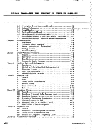
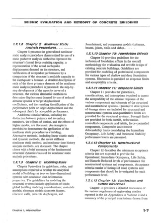
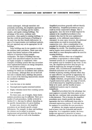
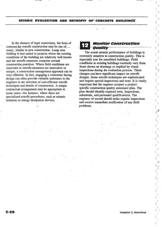
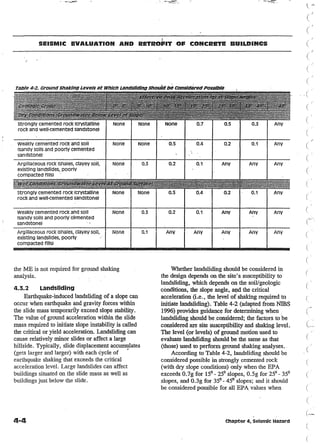
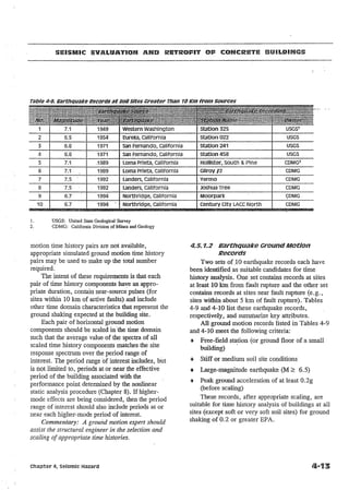
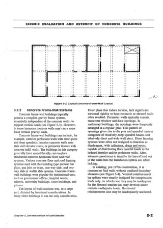
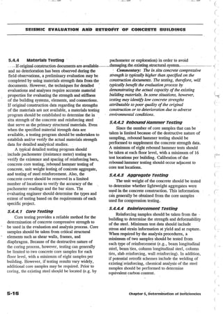
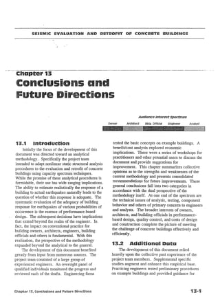
1. Simply apply a single concentrated
horizontal force at the top of the structure.
(Would generally only apply to a one-story
building.)
(2.) Apply lateral forces to each story in
--/
proportion to the standard code procedure
without the concentrated F, at the top (i.e.,
F, = [wrhx/Lwxhx]V).
/~1 Apply lateral forces in proportion to the
product of story masses and first mode
shape of the elastic model of the structure
(i.e., F, = [wxlf>x/Lwxt/Jx]V). The capacity
curve is generally constructed to represent
the first mode response of the structure
based on the assumption that the
fundamental mode of vibration is the
predominant response of the structure.
This is generally valid for buildings with
fundamental periods of vibration up to
about one second.
,> . . ~ ':
4. Same as Level 3 until first yielding, For
each increment beyond yielding, adjust the
forces to be consistent with the changing
deflected shape.
5.. Similar to 3 and 4 above, but include the
effects of the higher modes of vibration in
determining yielding in individual
structural elements while plotting the
capacity curve for the building in terms of
first mode lateral forces and
displacements. The higher mode effects
may be determined by doing higher mode
pushover analyses (i.e., loads may be
progressively applied in proportion to a
mode shape other than the fundamental
mode shape to determine its inelastic
behavior.) For the higher modes the
structure is being both pushed and pulled
concurrently to maintain the mode shape.
4. Calculate member forces for the required
combinations of vertical and lateral load.
5. Adjust the lateral force level so that some
el~rr:ent (or group of.elements) is stressed to j_
Within 10 percent of Its member strength.
. <,-.,
.-"
-c
U
J
-.
I
Chapter 8, Nonlinear Static Analys&s Procedures
Commentary: The element may be, for
example, a joint in a moment frame, a strut in
a braced frame, or a shear wall. Having
reached its member strength, the element is
considered to be incapable of taking additional
lateral load. For structures with many
elements, tracking and sequencing the analysis
at each and every element yield is time
consuming and unnecessary, In such cases,
elements should be grouped together at similar
yield points. Most structures can be properly
analyzed using less than 10 sequences, with
many simple structures requiring only 3 or 4.
6. Record the base shear and the roof
displacement.
Commentary: It is also useful to record
memberforces and rotations because they will
be needed for the performance check.
7. Revise the model using zero (or very small)
stiffness for the yielding elements. /
8. Apply a new increment of lateral load to the
revised structure such that another element (or
group of elements) yields.
Commentary: The'actual forces and
rotations for elements at the beginning of an
increment are equal to those at the end of the
previous increment. However, each application
of an increment of lateral load is a separate
analysis which starts from zero initial
conditions. Thus, to determine when the next
element yields, it is necessary to add the forces
from the current analysis to the sum of those
from the previous increments. Similarly, to
determine element rotations, it is necessary to
add the rotations from the current analysis to
the sum of those from the previous increments.
9. Add the increment of lateral load and the
corresponding increment of roof displacement
to the previous totals to give the accumulated
values of base shear and roof displacement.
10. Repeat steps 7, 8 and 9 until the structure
reaches an ultimate limit, such as: instability
from P-.6. effects; distortions considerably
beyond the desired performance level; an
element (or group of elements) reaching a

160. (
SEISMIC EVALUATION AND RETROFIT OF CONCRETE BUILDINGS
:
(
(
(
lateral deformation level at which significant
strength degradation begins, as defined in
Section 9.5; or an element (or group of
elements) reaching a lateral deformation level
at which loss of gravity load carrying capacity
occurs, as defined in Section 9.5. See
Figure 8-1 for a typical capacity curve.
Commentary: Some engineers.prefer to
continue the construction of the capacity curve
beyond the above suggested stopping points to
understand the structural behavior assuming
that all inadequate elements are retrofitted.
Exception: In certain cases where
elements lose all or a significant portion of
their lateral load carrying ability, but could
continue to deflect with no other
unacceptable affects, continuation of the
analysis may be justified. The most
notable example of this behavior may be
coupling spandrels in shear walls that are not
needed for vertical load support. This
behavior, which implies considerable
redistribution of lateral load, can be explicitly
modeled as indicated in step 11. This
procedure can also be used to'model elements
that degrade more gradually, but modeling this
behavior requires an estimation of the number
of cycles of loading, consideration of the
reliability of predicted behavior, and careful
review of all aspects of performance of the
degrading elements.
11. Explicitly model global strength degradation..
If the incremental loading was stopped in step
10 as a result of reaching a lateral deformation
level at which all or a significant portion of an
element's (or group of elements) load can no
longer be resisted, that is, its strength has
significantly degraded, then the stiffness of
that element(s) is' reduced, or eliminated, as
indicated in Section 9.5. A new capacity curve
is then created, starting with step 3 of this
step-by-step process. Create as many
Yield point for element
or group of elemen1s
(
I-
·as
CD
(
.c
tJ)
CD
UJ
as
m
(
Capacity curve
(
(
Roof Displacement
(::
(
Figure 8-1. capacity curve
(
(
I
First point of significant
strength degradation.
Stop capacity curve #1 at
this point. revise model to
reflect degraded
elements and start new
capacity .curve, capacity
Cf,Jrve#2..
Point at which
structure as modeled
for capacity curve #3
reaches an ultimate
limit, such as,
instability; excessive
distortions, or an
element (or group of
elements) reaching a
lateral deformation
level at which loss of
gravity load carrying
capacity occurs. Stop
curve at this point. "
(
‫­ן‬
m
.c
CD
First point of significant strength
degradation in capacity
curve #2. Stop curve at this
point, revise model to reflect
newly degraded elements and
start new capacity curve,
capacity curve #3.
fI)
CD
UJ
m
OJ
Roof Displacement
(
(
Figure 8-2. Multiple Capacity Curves Required To
Model strength Degradation
additional pushover curves as necessary to
adequately define the overall loss of strength.
Figure 8-2 illustrates the process, for an
example where three different capacity curves
are required.
Plot the final capacity curve to initially
follow the first curve, then transition to the
second curve at the displacement
corresponding to the initial strength
degradation, and so on. This curve will have a
"sawtooth" shape, as shown in Figure 8-3.
(
(
(
(
(
(
(
8-6
Chapter 8 Nonlinear static Analysis procedures
7
(

161. SEISMIC EVALUATION AND RETROFIT OF CONCRETE BUILDINGS
Degraded "sawtooth"
capacity curve shown
with solid line
I-
co
~
~
:«---------Ceapac;ly curve 113
,.,.;.;.,.,_,_:,':,./
Capacity curve #2
Capacity curve #1
Roof Displacement
Figure B-$. capacity curve With Global strength
Degradation Modeled
Commentary: Modeling global strength
degradation requires considerable judgment. If
strength degradation of over 20 percent is
explicitly modeled. then the actual expected
behavior of the degrading elements should be
carefully reviewed. In addition, the sensitivity
of the estimated demand displacement to the
modeling assumptions should be checked by
bounding the response with a range of
assumptions.
8.2.2
step By step Procedures To
Determine Demand
Commentary: Development of a capacity curve
for an existing building, in itself, is extremely
useful to the engineer, and will yield insights into
the building's performance characteristics as well
as methods of retrofit. However, to judge acceptability for a given Performance Objective, either
for the as-is condition or for a retrofit scheme, the
probable maximum displacement for the specified
ground motion must be estimated. Although a
significant amount of effort has been expended in
the last few years to develop simplified methods for
estimating this displacement (for this project, for
FEMA-273 (ATC 1996a), for LA's Division 95
(COLA 1995), for analysis of new isolated and
highly damped buildings, and in private
universities), no clear consensus has emerged.
Chapter 8, Nonlinear static Analysis Procedures
The project team for this document has
concentrated on the capacity spectrum method,
primarily because the method involves continued
and significant use of the capacity curve and
because of the potential ofthe method to assist
development of retrofit strategies, as shown in
Chapter 6. In addition, recent unpublished studies
at the State University ofNew York. Buffalo
(SUNY) indicate that the principles of the capacity
spectrum method. when combined with spectral
reductions based on estimates of hysteretic
damping similar to those used in this chapter, yield
displacements generally within 10 percent of the
average maximums from multiple time history runs.
The method of obtaining a design displacement
derivedfor the FEMA-273 document based on
application of coefficients to the elastic
displacement is also given as another option.
Considering the many possible variations in
ground motions, material properties, and
mathematical modeling of structural elements.. the
differences between results from this method and
the capacity spectrum method in the majority of
cases are insignificant. As in all aspects of
structural engineering, particularly when dealing
with existing buildings, good engineering judgment
must be exercised.
It is expected that in the near future, a
consensus will develop on this aspect ofsimplified
nonlinear analysis, which in combination with
computerized calculation of the capacity curve,
will enable development offar more cost-effective,
production-oriented procedures.
In order to determine compliance with a given
performance level, a displacement along the
capacity curve must be determined that is
consistent with the seismic demand. Two
methodologies for determining this displacement
are presented in this section.
The capacity spectrum method is presented in
Section 8.2.2.1. It is based on finding a point on
the capacity spectrum that also lies on the
appropriate demand response spectrum, reduced
for nonlinear effects. and is most consistent in
terms of graphical representation and terminology
with the balance of this document.

162. SEISMIC E'VAILUAT'IO'N' AND RETROFIT OF CONCRETE BUILDINGS
(
:
(
Extend initial stiffness line up to
intersect elastic response spectrum.
Read elastic spectral displacement,
d elasli et as ordinate of intersection point.
The Equal Displacement Approximation
estimates that the inelastic spectral
displacement is the same as that which
would occur if the Structure remained
perfectly elastic.
Elastic response spectrum
(5% damped)
" •d
= delaslic = d inelastic
Spectral Displacement
Figure 8-4. Equal Displacement Approximation
The demand displacement in the capacity
spectrum method occurs at a point, on the capacity
spectrum called the performance point, This
performance point represents the condition for
which the seismic capacity of the structure is equal
to the seismic demand imposed on the structure by
the specified ground motion.
The method used in FEMA-273 (ATe 1996a),
sometimes called the coefficient method, is
presented in Section 8.2.2.2. The coefficient
method is based on statistical analysis of the
results of time history analysis of single degree of
freedom models of different types. The demand
displacement in the coefficient method is called the
target displacement.
Commentary: An estimate of the displacement
due to a given seismic demand may be made using
a simple technique called the equal displacement
approximation. As shown in Figure 8-4, this
approximation is based on the assumption that the
inelastic spectral displacement is the same as that
which would occur if the structure remained
perfectly elastic. In some cases, particularly in the
longer period range (T> 1.0 seconds), the simple
equal displacement approximation will usually
yield.results similar to the capacity spectrum and
coefficient methods. In other cases, particularly in
the short period, range (T < 0.5 seconds) the
displacements obtainedfrom the simple
approximation may be significantly different from
(less than) the results obtained using the capacity
spectrum and coefficient methods.
The equal displacement approximation is often
a useful tool for estimating an initial trial
performance point in the iterative capacity
spectrum procedures described in Sections
8.2.2.1.2 and 8.2.2.1.3.
The target displacement obtained using the
displacement coefficient method is equal to the
displacement obtained using the equal
displacement approximation modified by various
coefficients.
8.2.2. '1 Calculating Demand using the
capacity spectrum Method
The location of the Performance Point must
satisfy two relationships: 1) the point must lie on
the capacity spectrum curve in order to represent
the structure at a given displacement, and 2) the
point must lie on a spectral demand cl:lrve, reduced
from the elastic, 5 percent-damped design
spectrum, that represents the nonlinear demand at
the same structural displacement. For this
methodology, spectral reduction factors are given
in termsof effective damping. An approximate
effective damping is calculated based on the shape
of the capacity curve, the estimated displacement
demand, and the resulting hysteresis loop.
Probable imperfections in real building hysteresis
loops, including degradation and duration effects,
are accounted for by reductions in theoretically
calculated equivalent viscous damping values.
In the general case, determination of the
performance point requires a trial and error search'
for satisfaction of the two criterion specified
above. However, this section contains three
different procedures that standardize and simplify
this iterative process. These alternate procedures
are all based on the same concepts and
mathematical relationships but vary in their
(
(
(
(
(
,1.
(
j~
(
(
(
(
(
(
8·8
Chapter S, Nonlinear st~tic Analysis Procedures
(
(

163. SEiSMIC EVALUATION AND RETROFIT OF CONCRETE BUiLDINGS
.:
dependence on analytical versus graphical
techniques. This section is organized as follows:
.. Conceptual Development of the Method
(Section 8.2.2.1.1). This section contains the
theoretical basis of the method and the
derivation of formulae. Considerable, and
careful, study by the user is required to digest
the background theory presented in this
section. This section is not intended to serve as
step by step instructions for determination of
the performance point. For such step by step
instructions, the user should proceed to
Procedure A, B, or C , in which only the
minimum required mathematical relationships
of this section are referenced.
•
..
~
Procedure A (Section 8.2.2.1.2). This is the
most direct application of the concepts and
relationships described in Section 8.2.2.1.l.
Procedure A is truly iterative, but is
formula-based and easily can be programmed
into a spreadsheet. It is more an analytical
method than a graphical method. It may be the
best method for beginners because it is the
most direct application of the methodology,
and consequently is the easiest procedure to
understand.
Procedure B (Section 8.2.2.1.3). A
simplification is introduced in the bilinear
modeling of the capacity curve that enables a
relatively direct solution for the performance
point with little iteration. Like Procedure A,
Procedure B is more an analytical method than
a graphical method, and it is probably the most
convenient for spreadsheet programming.
Procedure B may be a less transparent
application of the methodology than
Procedure A.
Procedure C (Section 8.2.2.1.4). Procedure
C is a pure graphical method to find the
performance point, similar to the originally
conceived capacity spectrum method, and is
consistent with the concepts and mathematical
relationships described in Section 8.2.2.1.1. It
is the most convenient method for hand
Chapter 8, Nonlinear static A.nalysis Procedures
analysis. It is not particularly convenient for
spreadsheet programming. It is the least
transparent application of the methodology.
Commentary: Users who study the three
procedures above will have a good understanding
of the capacity spectrum method, and will
probably have their preferred procedure.
However, other mathematical or graphical
procedures may also be developed to provide a
better interface with a user's other analytical
methods.
8.2.2.1.1 Conceptual Development of the
Capacity Spectrum Method
Conversion of the Capacity Curve to the
Capacity Spectrum
To use the capacity spectrum method it is
necessary to convert the capacity curve, which is
in terms of base shear and roof displacement to
what is called a capacity spectrum, which is a
representation of the capacity curve in
Acceleration-Displacement Response Spectra
(ADRS) format (i.e., Sa versus Sa). The required
equations to make the transformation are:
N
"LC-Wi¢il) I g
PFl=
i=l
N
(8-1)
"L(Wi¢~l) I g
i=1
(8-2)
Sa = V IW
(8-3)
(Xl
A root
Sd=---PF 1 rproot.1
(8-4)

164. SEISMIC EVALUATION AND RETROFIT OF CONCRETE BUII.DINGS
PF 1«proof,1 = 1.6
~~~Arom
v = aSaW
PF1«proof,1 = 1.4
~rom
a=O.7
a=O.8
PF1«proof,1 = 1.2 PF1«proof,1 = 1.0
~rom
a=O.9
Amm
a= 1.0
Figure 8-5. Example Modal participation Factors and Modal Mass CoeFFicients
where:
PFl= modal participation factor for the
first natural mode.
modal mass eoefficient for the first
natural mode.
= mass assigned to level i.
Wi /g
€Pil = amplitude of mode 1 at level i.
N = level N, the level which is the
uppermost in the main portion of
the structure.
V = base shear.
W = building dead weight plus likely
live loads, see Section 9.2.
roof displacement (V and the
associated 6.roof make up points on
the capacity curve).
Sa = spectral acceleration.
Sa = spectral displacement (Sa and the
associated Sa make up points on
the capacity spectrum).
Section 8.5 provides general information on
structural dynamics and more information on the
derivation of these equations. It is helpful to have
some physical understanding of the relationship
between the participation factor, the modal mass
coefficient, and building displacement. As shown
in Figure 8-5, the participation factor and the
modal mass coefficient vary according to the
relative interstory displacement over the height of
the building. For example, for a linear distribution
of interstory displacement oyer the height of the
building, <X == 0.8. and PFl<Proof.l == ~ .4.
The general process for converting the
capacity curve to the capacity spectrum, that is, .
converting the capacity curve into the ADRS
format, is to first calculate the modal participation
factor PFI and the modal mass coefficient <Xl using
equations 8-1 and 8-2. Then for each point on :the
capacity curve, V, '&-oof, calculate the associated
point Sa, Sa on the capacity spectrum using
equations 8-3 and 8-4.
Most engineers are familiar with the traditional
Sa versus T representation of response spectra;
however, they are less familiar with the Sa versus
Sd (ADRSr representation. Figure 8-6 shows the
same spectrum in each format. In the ADRS
format, lines· radiating from the origin have
constant period. For any point on the ADRS
spectrum, the period, T, can be computed using
the relationship T=2n(SdiSa)ll2. Similarly, for any
point on the traditional spectrum, the spectral
t.
(
(
(
(
(
(
8-10
Chapter 8, Nonlinear static Analysis Procedures
(

165. SEISMIC EVALUATION AND RETROFIT OF CONCRETE BUILDINGS
;
In ADRS format,
lines radiating from
the origin have
constant periods.
C
I-----t--- ----------------------- ----- ----0 - - ! - - - J .
.
Z
as
"oeD
iii
U
u
________________________________0;;(.
_
n;
--------------------0.- - ---- -----------------=""--Q)
I-
Co
en
Spectral Displacement
ADRS Spectrum
(Sa versus Sd)
Traditional Spectrum
(Sa versus T)
Figure 8-6. Response spectra in Traditional and ADRS Formats
Demand spectrum
I--..J..-.--t----------- - - -
--
- -00------ __
C
;g -+---1---/
E
eD
iii
u
_ B
.:l
:.; _~~
__......
Spectral Displacement
Traditional Spectrum
(Sa versus T)
ADRS Spectrum
(Sa versus Sd)
Figure 8-7. capacity spectrum superimposed over Response spectra in Traditional and ADRSFormats
disp lacement, Se, can be computed using the
relationship Sd=SaT2 /4n 2 • These two relationships
are the same formula arranged in different ways.
Figure 8-7 shows the same capacity spectrum
superimposed on each of the response spectra plots
shown in Figure 8-6. Following along the capacity
spectrum, the period is constant, at T 1, up until
Chapter 8, Nonlinear static Analysis Procedures
point A. When point B is reached, the period is
T 2. This indicates that as a structure undergoes
inelastic displacement, the period lengthens. The
lengthening period is most apparent on the
traditional spectrum plot, but it is also clear on the
ADRS plot, remembering that lines of constant
period radiate from the origin.

166. SEISMIC EVALUATION AIYD RETROFIT OP CONCRETE BUILDINGS
:
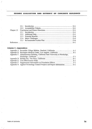
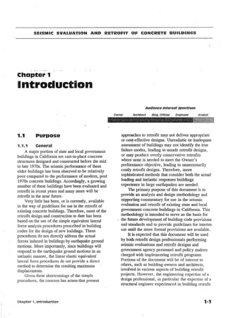
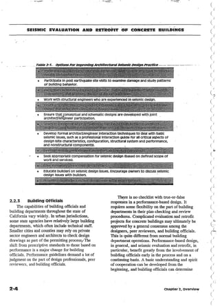
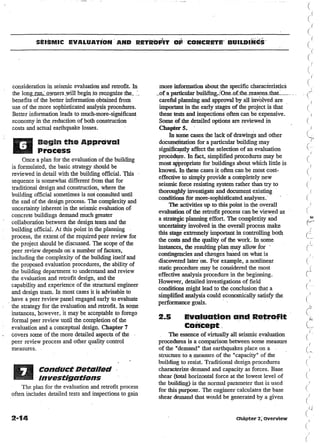
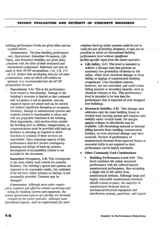
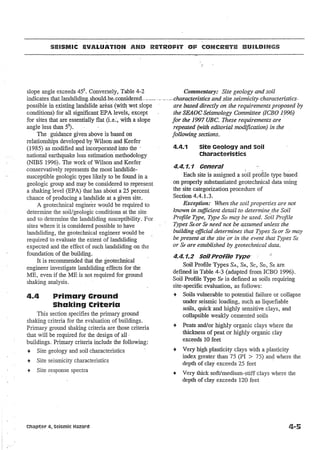
Conversion to ADRS Spectra
Application of the Capacity-Spectrum technique requires that both the demand response
spectra and structural capacity (or pushover) curves be plotted. in the spectral acceleration
vs. spectral displacement domain. Spectra plotted in this format are known as
Acceleration-Displacement Response Spectra (ADRS) after Mahaney, 1993.
Every point on a response spectrum curve has
associated with it a unique spectral acceleration, Sa'
Sa
spectral velocity, Sy7 spectral displacement, Sd and
I
period, T. To convert a spectrum from the standard
J
I
Sa vs T format found in the building code to ADRS
I
I
format, it is necessary to determine the value of
-----.,-----IJ
I
Sdi for each point on the curve, Sai'~' This can be
To
1i
done with the equation:
Standard Format (Sa vs T)
];2
= - L - Sn.g
f
411: 2 .,
/'To
Sa
1----'1
(
(
('
(
s,
1
1
1
1
Sai
1
- -
-1-
1
_
1
--
'""-'-
--
--.,.---_..P.'d
Sdi
Standard demand response spectra contain a
range of constant spectral acceleration and a
second range of constant spectral velocity.
Spectral acceleration and displacement at period
T, are given by:
ADP..s Fermat (Sa Vii Sil)
SalK =
2n-s."
11
Sdi
1;
=-s."
2n-
s:::
In order to develop the capacity spectrum from
o the capacity (or pushover) curve, it is necessary
"iii to do a point by point conversion to first mode
;,..
C1)
:> spectral coordinates. Any point Vi, 4001 on the
capacity curve is converted to the corresponding
(J point Sai Sdi on the capacity spectrum using
E the equations:
.i
(
(.
(
S
(
!
o
s
{Ii
RoofDisplacement - 4-
(
s - Il roofI
2
Q)
~
·u
co
=ViIW/
;fa!
ai
di -
/
Capacity Curve
(PE;. X If'l,roo! )
where a 1 and PF1 are respectively the modal mass
coefficient and participation factors for the first
(J natural mode of the structure and <I> l,roof is the roof
level amplitude of the first mode. See also Section
8.5, Basics of Structural Dynamics.
fa-
Spectral Displacement - Sd
Capacity Spectrum
(
(
(
(
8-12
Chapters. Nonlinear static Analysis procedures
(

167. Note:
1. K( = Initial Stiffness
2. Area A 1 = Area A2
Basic Equation
T=21t'/Sd'Sa
Point 1
1.0...---..--.-/----.--...,
m0.8-1---.,.....--1----1
Sa=O.8
Sd=1.95
T=21t'r-:-.""'"=""..,...,0 .B *:""'3 6.'""'" = 0.50 sec
"'""'
1" 95 """' : :=a= 4
~
Point 2
o
Sa=0.S2
Sd=1.29
T=21tJ"'""i.-=29=-1"'-:0'-:.5=2-=*-=38=6~.4 = 0.50 sec
:;:;
~ 0.6;+--_1-l--'.--l--~-1
Q)
ai
o
~ O.4-1---I-++--~~=---1
Point 3
Sa=O.4
Sd=3.95
T=21tJ=3-::=.9'='"S..,.."0==-.4-=-=-"3=8=6"""".4 = 1.00 sec
"'li1i
t) O.2+-1--~-----.:::::....,..+_-_+_-.=-.-.=----,------,
Q)
0-
W
O.O~--l---+_-_+_--+--_+_----l
o
2
4
6
8
10
12
i
c ap'4-- - - f - - - - -
.2
11
:D.
iiy
Qi
o
o
<C
i1inear Representaf n
Capacity Spectrum
m
aU
Q)
Co
rn
. dy
dpl
Spectral Displacement
Figure 8-9_ Bilinear Representation of capacity
spectrum For capacity Spectrum Method
Spectral Displacement (inches)
Figure 8-8. Lines of Constant Period and period
Lengthening in ADgS Format
Figure 8-8 helps illustrate that, in the ADRS
format, lines radiating from the origin have
constant period, and that the period lengthens as
the structure undergoes inelastic displacement.
Points 1 and 2 in the figure lie on two different
response spectra, and on a single line radiating
from the origin. As shown by the calculation
included in the figure, they both are associated
with a period of 0.5 seconds. Point 3 has a 1.0
second period. Thus, for the capacity spectrum
(pushover) shown, the elastic period of the
structure is 0.5 seconds, and when the structure is
pushed to point 3, with a spectral displacement of
3.95 inches, and considerable inelastic
displacement, the period has lengthened to 1.0
seconds.
Construction of Bilinear Representation of
Capacity Spectrum
A bilinear representation of the capacity
spectrum is needed to estimate the effective
damping and appropriate reduction of spectral
demand.' Construction of the bilinear representation requires definition of the point api, dpi. This
point is the trial performance point which is estimated by the engineer to develop a reduced
demand response spectrum. If the reduced response spectrum is found to intersect the capacity
Chapter 8, Nonlinear: static Analysis procedures
Note:
1. ~ = Initial Stiffness
2. Area A 1 = Area A 2
Bilinear representation
based on capacity
spectrum associated
with the point api' d pl
dy
dp1
Spectral Displacement
Figure 8-10. Bilinear eepresentation of capacity
spectrum for oegrading trsswtoottt") system
spectrum at the estimated api, dpi point, then that
point is the performance point. The first estimate
of point api, dpi is designated apI, dpI, the second
ap2, dp2, and so on. Guidance on a first estimate of
point apI, dpl is given in the step-by-step process
for each of the three procedures. Oftentimes, the
equal displacement approximation can be used as
an estimate of ap 1, dp l.
Refer to Figure 8-9 for an example bilinear
representation of a capacity spectrum. To

168. SEISMIC EVALUATION AND RETROFIT OF CONCIlETE BUILDINGS
:
(
l·'
ED
= Energy dissipated by damping
= Area of enclosed by hysteresis loop
=Area of parallelogram
Bilinear representation
of capacity spectrum
Eso = Maximum strain energy
= Area of hatched triangle
= 8ptdpl/2
(
Po = Equivalent viscous damping
(
assocciated with full
hysteresis loop area
=_1 ~
41t Eso
Figure 8-11. Derivation of Damping For spectral Reduction
construct the bilinear representation draw one line
up from the origin at the initial stiffness of the
building using element stiffnesses as recommended
in Chapter 9. Draw a second line back from the
trial performance point, api, dpi. Slope the second
line such that when it intersectsthe first line, at
point ay, dy, the area designated Ai in the figure is
approximately equal to the area designated A2,
The intent of setting area A: equal to area A2 is to
have equal area under the capacity spectrum and
its bilinear representation, that is, to have equal
energy associated with each curve.
In the case of a "sawtooth" capacity spectrum,
the bilinear representation should be based on the
capacity spectrum curve which describes behavior
at displacement dpi, as shown in Figure 8-10.
Estimation of Damping and Reduction of
5 percent Damped Response Spectrum
The damping that occurs when earthquake
ground motion drives a structure into the inelastic
range can be viewed as a combination of viscous
damping that is inherent in the structure and
hysteretic damping. Hysteretic damping -is related
to the area inside the loops that are formed when
the earthquake force (base shear) is plotted against
8.,,14
the structure displacement. Hysteretic damping can
be represented as equivalent viscous damping
using equations that are available in the literature.
The equivalent viscous damping, {3eq,
associated with a maximum displacement of dpi,
can be estimated from the following equation:
(3eq = (30 + 0.05 .
(8-5)
where,
(30 = hysteretic damping represented as
equivalent viscous damping
0.05 = 5% viscous damping inherent in the
structure (assumed to be constant)
The term (30 can be calculated as (Chopra 1995):
/30 = _1_
ED
(8-5a)
4n Eso
where,
ED= energy dissipated by damping
Es o = maximum strain energy
The physical significance of the terms ED and
Es o in equation 8-5a is illustrated in Figure 8-11.
Chapter 8, Nonlinear static Analysis procedures
(

169. SEISMIC EVALUATION AND RETROFIT OF CONCRETE BUILDINGS
:
ED = Area of enclosed by hysteresis loop
= Area of large parallelogram
= 4 times area of shaded parallelogram
C"
o
;; Elpi
Formulas for designated areas:
A 1 = (api -
c
o
~
E ~----GJ
(Day
ay) . . dy
A2 = (ay . . d y) /2
A3 = [(~ - ay) . . (d pi - d y ) ]
C!p1-r--- -.-- - - - - - - '"=1
ba
CD
ai
Co)
e
ay-l----I~
o
<C
ca
J..
.....
e
Q)
a.
en
dy.
Spectral Displacement
Figure 8-12.. Derivation of Energy Dissipated by
Damping, ED
ED is the energy dissipated by the structure in a
single cycle of motion, that is, the area enclosed
by a single hysteresis loop. Es o is the maximum
strain energy associated with that cycle of motion,
that is, the area )f the hatched triangle.
Referring to Figures 8-11, 8-12 and 8-13, the
term ED can be derived as
ED = 4*(shaded area in Figures 8-12 or 8-13)
= 4(apidpi - 2Al - 2Az - 2A3)
= 4[apidpi-aydy-(dpi-dy)(api-ay) - 2dy(CIpi- ay)]
= 4(aydpi - dyapi)
Referring to Figure 8-11, the term Eso can be
derived as
Es o = apidpi /2
Commentary: Note that Es; could also be
written as keffectivedp//2.
Thus , ~o can be written as:
f3 0 = _.1_ 4 (aydpi - dyapi) = ~ aydpi - dyapi
471:
apidpi
[30 = O.637(a ydp i
-
/2
71:
apidpi
dyapi)
apidpi
Chapter 8, Nonlinear static Anarysis procedures
Figure 8-1$. Derivation of Energy Dissipated by
Dampingl ED
and when ~o is written in terms of percent critical
damping, the equation becomes:
130 =
63.7(a yd pi - dyapi)
apidpi
(8-6)
Thus (3eq becomes:
~eq = (30 +5 = 63.7(aydpi
-
dyapi)
+5
(8-7)
apidpi
The equivalent viscous damping values
obtained from equation 8-7 can be used to estimate
spectral reduction factors .using relationships
developed by Newmark and Hall [Newmark and
Hall, 1982]. As shown in Figure 8-14, spectral
reduction factors are used to decrease the elastic
(5 % damped) response spectrum to a reduced
response spectrum with damping greater than 5 %
of critical damping. For damping values less than
about 25 percent, spectral reduction factors
calculated using the (3eq from equation 8-7 and
Newmark and Hall equations are consistent with
similar factors contained in base isolation codes
and in the FE1'4A Guidelines (these factors are
presented in these other documents as the damping
coefficient, B, which is equal to l/SR, see the
commentary below). The committees who

170. (-
(
SEISMIC EVALUATION AND RETROFIT OF CONCRETE BUILDINGS
:
(
(
-.
Notes: 1. See Chapter 4 for CA and Cv values.
2. SR A is spectral re'duction value in
constant acceleration range of spectrum.
3. SR v is spectral reduction value in
constant velocity range of spectrum.
c
o
';:l
e
~
CJ
SR"C,/T= Cv!(TBJ
~ CA
E
'0
Q)
a.
en
Reduced response
spectrum
Spectral Displacement .
Figure 8-14. Reduced Response spectrum
developed these damping coefficients concluded
that spectra should not be re~lJ.ced to this extent at
higher damping values and judgmentally increased
the coefficients starting at about 25 percent the
damping (increasing the damping coefficient B is
the same as decreasing the spectral reduction
factor SR, the net result is that the spectra are
reduced less), as well as set an absolute limit on
reductions at a ~eq of about 50 percent.
Commentary: This document is written using
the concept of spectral reduction factors, SR.
However, both the term spectral reduction (SR)
and the term damping coefficient (8 = LlSR) are
carried through this section. The term spectral
reduction factor has been used widely in the
literature and previously in this project, but B,
damping coefficient, is currently in use in other
codes such as the 1991 UBC, 1994 UBC, FEMA
Guidelines and 1994 NEHRP Provisions. The
damping coefficient B, which is used to reduce the
elastic (5 % damped) spectrum, should not be
confused with the damping, 13. The damping
coefficient is derived from a formula which
includes the variable, f3.
8-16
The idealized hysteresis loop shown in Figure
8-11 is a reasonable approximation for a ductilely
detailed building subjected to relatively short
duration ground shaking (not enough cycles to
significantly degrade elements) and with equivalent
viscous damping less than approximately 30 %.
For conditions other than these, the idealized
hysteresis loops of Figure 8-11 lead to
overestimates of equivalent viscous damping
because the actual hysteresis loops are imperfect,
that is, they are reduced in area, or pinched.
This document addresses existing reinforced
concrete buildings that are not typically ductile
structures. For such buildings, calculation of the
equivalent viscous damping using equation 8-7 and
the idealized hysteresis loop in Figure 8-11 yields
results that overestimate realistic levels of
damping. In this document, in order to be
consistent with these previously developed
damping coefficients, B, as well as to enable
simulation of imperfect hysteresis loops (loops
reduced in area), the concept of effective viscous
damping using a damping modification factor, x,
has been introduced. Effective viscous damping,
~ff, is defined by:
R
R +5 - 63.7"x::(a ydpi - dyapi)
(8-8)
p~-~o
+5
(~
apidpi
Note that equation 8-8 is identical to equation
8-7 except that the lC- factor has been introduced to
modify the first (~o) term.
The x-factor is a measure of the extent to
. which the actual building hysteresis is well
represented by the parallelogram of Figure 8-11,
either initially, or after degradation. The x-factor
depends on the structural behavior of the building,
which in tum depends on the quality of the seismic
resisting system and the duration of ground
shaking. For simplicity, this document simulates
three categories of structural behavior. Structural
behavior Type A represents stable, reasonably full
hysteresis loops most similar to Figure 8-11, and
is assigned a 1C of 1.0 (except at higher damping
values as discussed above). Type B is assigned a
basic 1C of 2/3 and represents a moderate reduction
Chapter 8,. Nonlinear static Analysis procedures
(
(
(
(

171. SEiSMIC EVALUAT!@N AND RETROFIT OF CONCRETE BUILDINGS
of area (x is also reduced at higher values of peff to
be consistent with the Type A relationships). Type
C represents poor hysteretic behavior with a
substantial reduction of loop area (severely
pinched) and is assigned a K of 1/3.
The ranges and limits for the values of
lC assigned to the three structural behavior types
are given in Table 8-1 and illustrated in Figure 815. Although arbitrary, they represent the
consensus opinion of the product development
team. The value of K for structural behavior Type
A (good behavior), is derived from the spectrum
reduction factors, B, specified in the" Uniform
Building Code (leBO 1994) and the NEHRP
Provisions (ESSe 1995) for the design of new base
isolated buildings. The values of lC assigned to the
other two types are thought to be reasonable for
average and poor structural behavior. The
numerical derivation of spectral reduction factors
used in this methodology, based on these assigned
values of K, follows.
Table 8-1. Values for Damping Modification Factor,
>16.25
1.13 _ 051(a yd p i
-
dyapi)
apidpi
Type B
~25
0.67
0.845 0.446(a ydpi
>25
dyapi)
-
apidpl
rvoe c
1.
2.
Any value
0.33
See Table 8-4 for structural behavior types.
The formulas are derived from Tables of spectrum reduction
factors, B (or BI), specified for the design of base isolated
buildings in the 1991 UBC, 1994 UBC and 1994 NEHRP
Provisions. The formulas created for this document give the same
results as are in the Tables in the other documents.
Numerical Derivation of Spectral Reductions
The equations for the reduction factors SRA
(equal to lIBs) and SRv (equal to l/BL) are given
by:
SRA
Table 8-2. Minimum Allowable SRA and SRv
vstuest
= ~::
3.21- O.68ln(f3eff)
(8-9)
Bs
2.12
3.21- o.68In[63.77C(aydpi - dyapi) +
apidpi
2.12
2 Value in Table 8-2
rvpes
1.
2.
0.44
0.56
TypeC
5]_
SRv = _1 :: 2.31 - 0.41ln(f3eff)
BL
1.65
2.31- 0.4lln[63.77C(aydpi - dyapi)
apidpi
0.56
0.67
Values for SRA and SRv shall not be less than those
shown in this Table
See Table 8-4 for structural behavior types.
(8-10)
+
5]
= -----=--------=
1.65
2 Value in Table 8-2
Note that the values for SRA and SRv should be
greater than or equal to the values given in
Table 8-2.
Chapter 8, Nonlinear static Analysis Procedures
K:
To illustrate the effect of the structural
behavior types on the spectral reduction factors,
Figures 8-15, 8-16, 8-17 and 8-18 respectively
show graphical representations of 7<:, f3eff, SRA and
SRv versus po for structural behavior types A, B
and C. Note that ~o is the equivalent viscous
damping representation of the hysteretic damping
associated with the full area of the hysteresis loop
formed by the bilinear approximation of the
capacity spectrum, as shown in Figure 8-11.

172. (
SEISMIC EVALUATION AND RETROFIT OF CONCRETE. BUILDINGS
:
, --~
ci 0.90
I
(j O.SO
ca
Structural
Behavi~rT''DeB:
-
I
+:
I
~ 0.50
~
--
-:
- ---
~
10
0
16.25 20
25
."t@J'
. [ 25
:;:::;
Co)
Q)
in
»:
3D
-:
20
15
10
5
o
~,
~·rif:seha ~iorTVp.n
45
40
30
50
60
~
0.00
o
30
10
40
45
50
Hysteretic Damp~ng Represented As
Equivalent Viscous Damping, ~D (%)
Figure 8-18. spectral eeaucttonFactor, sev., for
structural Behavior Types A, Band C
to.
:a 35
~
----
---Stru ~raI!BehaIIlorTypeC
-- ... -- ;;----;.
0.20
a:
0.00
40
C
-----
~ ---
Q)
Figure 8-15. Damping Modification Factor, 1(, for
structural Behavior Types A, Band C
~
<,
.
0.40
(j
Hysteretic Damping Represented As
Equivalent Viscous Damping, /30 (%)
~
0.60
c
o
Q)
C
en
:g
I~:: . ro ____
:::I
Q. 0.10
co..
0.80
"C
en 0.20
~
I
tl.
'
~ 0.30
C
1.00
U
:
.
.................
..... ":
------ .. :.::~- --r-- -- --- - ---- -----
0.40
1.20
en
r-----
I
- - -- - -;- f- -: __
U. 0.70
C
o 0.60
~
rl
Structural Behavior Type A
~ 1.00
-:
/'
o
_
.....Js
r g ee't,!! ~
_
~"';"
"'"
c:.f'
Soil Profile Type
'';''':
~f!!'!':
=Sa
ZEN=OA
CA=OA
.I"I'''t~pec
./
/: -- -- --.e>
./
p
..~i5' ~l
Cv=0.4
.. - -!
63.7(l!ydp, -
dAJ
",,-
20
10
4fj
40
3D
50
60
Hysteretic Damping Represented As
Equivalent Viscous Damping, /30 (%)
Figure 8-16. Effective Damping, !3en, for structural
Behavior Types A, Band C
r::t
Spectral Displacement (inches)
1.00
en
1
.......
0.90
oS
0.80
~
0.70
..:
(,)
.§
',.....
",
"
(j 0.50
-6
0.40
a:
Figure 8-19. EXample ADRS Response spectra for
structural Behavior Types .A, Band C
- .. --
......
0.60
.....
-
--
~
:~~IJ~al
S
0.30
~
tr
ae ~a",...L,
c ____
__ .;.
ruetura'R.. . '
<:» ructura'&1 ;:.:;;:~~ l'L __
<, .......
Q)
e
o~~~~::±=±=jl
o
2
4
6
8
10
12
14
16
0.20
:..r!!~
---
_ '-':'YPe4
,
0.10
0.00
o
10
20
30
40
45
50
60
Hysteretic Damping Represented As
Equivalent Viscous Damping, /30 (%)
Figure 8-17. spectral Reduction Factor, SRA, for
structural Behavior Types A, Band C
BIlI18
Chapter 8, Nonlinear
static Analysis Procedures
GO

173. SEISliVUC eVALUATION AND RETROFIT. OF CONC-RETE BUiLDINGS
:
Table B·S. spectral Reduction Factors, SRA
=
1/Bs and sev
SRA
SRv
= 1/ Bt
SRA
J30 tpercenn
J3eff
(1/85)
(1/8tJ
J3eff
(1/85>
(1/8tJ
l3eff
(1/B5)
(1/BrJ
0
5
1.00
1.00
5
1.00
1.00
5
1.00
1.00
5
10
0.78
0.83
8
0.83
0.87
7
0.91
0.93
15
20
0.55
0.66
15
0.64
0.73
10
0.78
0.83
25
0.44
0.57
22
0.53
13
0.69
0.76
35
35
0.38
0.52
26
0.47
0.59
17
0.61
0.70
~45
1.
2.
28
0.63
40
0.33
0.50 2
29
0.44
0.56
20
0.56
0.67 2
Structural behavior type, see Table 8-4.
Controlled by minimum allowable value for SRv, see Table 8.2
Figure 8-19 shows the difference in the response
spectra in ADRS format for structural behavior
types A, B and C when {3o equals 15%.
The spectral reduction factors SRA (equal to
1/Bs) and SRv (equal to IIB 4) given in equations
8-9 and 8-10 can be put in tabular form as shown
in Table 8-3. Enter the Table with the parameter
130, the equivalent viscous damping representation
of the hysteretic damping associated with the full
area or the hysteresis loop formed by the bilinear
approximation of the capacity spectrum in Figure
8-11.
Commentary: The inverted value of BL for
structural behavior Type A is identical to the
damping coefficient used in other codes such as the
1991 UBe, 1994 UBC and 1994 NEHRP
Provisions.
The selection of structural behavior type
depends. on both the quality of the primary
elements of the seismic resisting system and the
duration of shaking, as shown in Table 8-4.
Criteria to determine the appropriate duration
category for a given situation are given in
Chapter 4 (Section 4.5.2). The first column of
structural behavior types, Essentially New
Buildings, represents buildings with new lateral
force resisting systems and detailing complying
with current code, in which the existing
Chapter 8, Nonlinear static Analysis procedures
Table 8-4. structural Behavior Types
Short
2.
3.
4.
Type 8
Type C
Long
1.
Type A
rvce s
Type C
Type C
See Section 4.5.2 for criteria.
Buildings whose primary elements make up an
essentially new lateral system and little strength or
stiffness is contributed by noncomplying elements.
Buildings whose primary elements are combinations of
existing and new elements, or better than average
existing systems.
Buildings whose primary elements make up
noncomplying lateral force systems with poor or
unreliable hysteretic behavior.
noncomplying elements contribute little strength or
stiffness. The third column of Table 8-4, Poor
Existing Buildings, represents existing buildings
with a lateral force resisting system with unlmown
or unreliable hysteretic behavior or behavior
known to degrade or be severely pinched. The
middle column, Average Existing Buildings, should
be used for other cases, and may be appropriate for
the majority of existing retrofit buildings.
Commentary: As described in Section 3.4, a
seismic performance objective is defined by
selecting a desired building performance level for a

174. SEISMIC EVAI.UATION AND RETROFIT OF CONCRETE BUII.DINGS
Pert of 5%, 10%, 15%,200/0, 25%, 30%, 35%, and
Soil Profile Type
ZEN 0.4
CA = 0.4
=
_
-
O.B
'ii
~
c(
0.4
8.
0.2
f
'0
en
2
12
~
~~
U
U
-
and 40%
Soil Profile Type = Sa
ZEN=OA
CA=OA
Cv=0.4
0.6
~
CD
fSatf of 5%, 10%. 150/0, 200/0, 25"'10, 30%, 35%,
40%
c,,~0.4
1.0
CD
c
o
=Se
"~
~ ~ ::---.
-~
0.0
o
0.5
1.5
2
-2.5
3
3.5
Period (seconds)
4.
4
6
8
10
14
Spectral Displacement (inches)
(
Figure 8-20. Family of Demand spectra in
Traditional sa versus TFormat
site. For example, a building may have short
duration shaldng for a Serviceability Earthquake
(usually 50% chance of being exceeded in 50
years) and long duration shaking for a Design
Earthquake (usually 1()% chance of being
exceededin 50 years). As another example, a
building may.have short duration shaking for the
maximum shaking expectedfrom a single event on
a one adjacent fault, and long duration shaldng for
the maximum shaking expectedfrom a single event
on another adjacent fault.
Development of the Demand Spectrum
The 5 percent response spectrum can be
developed based on the information in Chapter 4.
The reduced 5 percent response spectrum, called
the demand spectrum, can be plotted as shown in
Figure 8-14. A procedure for converting the
response spectrum from the standard Sa versus T
format to the Sa versus Sa format (ADRS) is given
near the beginning of Section 8.2.2.1.1.
Figure 8-20 depicts an example family of
demand spectra, each spectrum representing a
different level of effective damping, plotted in the
given level of earthquake ground motion. Dual- or
multiple-level performance objectives can be
created by selecting two or more different
performances, each for a different level of ground
Figure 8-21. Family of Demand spectra in ADRS
Format
motion. With multiple-level performance
objectives, it is possible, based on the criteria fat
duration of ground shaking given in Section 4.5.2,
to have short earthquake shaking duration for one
ground motion and long earthquake shaking
duration for another ground motion at the same
traditional Sa versus T format. Figure 8-21 shows
the same family of demand spectra, each spectrum
representing a different level of effective damping,
plotted in the ADRS format. Families of demand
spectra, such as these, can be plotted for any .
combination of soil profile type and earthquake
shaking intensity using the information provided in
Chapter 4. Such families of demand spectra,
plotted in the ADRS format, can be quite useful
when analyzing the structure using the capacity
spectrum method.
Intersection of Capacity Spectrum and
Demand Spectrum
When the displacement at the intersection of
the demand spectrum"and the capacity spectrum,
dt, is within 5 percent (O.95dpi ~ dr ~ 1.05 dpi) of
the displacement of the trial performance point,
api, dpi, dpi becomes the performance point. If the
intersection of the demand spectrum and the
capacity spectrum is not within the acceptable
(
(
(
(
(
8·20
Chapter 8, Nonlinear static Analysis procedures

175. SEISMIC EVALUATION AND RETROFIT OF CONCRETE BUILDINGS
:
tolerance, then a new api, dpi point is selected and
the process is repeated. Figure 8-22 illustrates the
concept. The performance point represents the
maximum structural displacement expected for the
demand earthquake ground motion.
When the capacity spectrum is a "sawtooth"
curve, that is, the [mal composite capacity
spectrum is constructed from several different
capacity spectra which account for strength
degradation of elements; special care must be
taken in determining the performance point. The
bilinear representation of the capacity spectrum,
that is used to determine the reduction factors for
the 5 percent damped spectrum, is constructed for
a single capacity spectrum curve, not the
composite curve. For the analysis to be acceptable,
the bilinear representation must be for the same
single capacity spectrum curve that makes up the
portion of the composite capacity spectrum where
the intersection point occurs. Figure 8-23
illustrates the concept for a "sawtooth" capacity
spectrum.
Intersection point of demand spectrum
and capacity spectrum
Note:
dpl trial perfromance point
d, = displacement intersection point
~,
d, ~
Spectral Displacement
Figure 8-22. Intersection point of Demand and
capacity spectrums Within Acceptable Tolerance
Commentary: If the performance point is
found to fall near a step in the "sawtooth" capacity spectrum, then the engineer should be aware
that, because of the variability of the analysis, the
actual building displacement could be on either
side of the step. The engineer should consider both
points when examining building performance.
Procedure A:
?
.. Clearest, most transparent and most direct
application of the methodology
.. Analytical method
.. Convenient for spreadsheet programming
.. May be the best method for beginners because it
is most direct and thus easiest to understand
----I
Procedure B:
Analytical method
.. Simpler than procedure A because of simplifying
assumptions (that may not always be valid)
.. Most convenient for spreadsheet programming
.. Reasonably transparent application of
methodology
• Users of this method should fully understand the
inherent assumptions
II
Question: Which
capacity spectrum
procedure should I use?
Answer: It largely
depends on personal
preference, but these
guidelines may help.
Procedure C:
..
•
•
..
Chapter 8, Nonlinear static Analysis Procedures
=
Graphical method
Most convenient method for hand analysis
Not as convenient for spreadsheet programming
Least transparent application of methodology

176. SEISMIC EVALUATION AND RETROFIT OF CONCRETE BUILD"ING"S
:
Intersection pointof demandspectrumand
capacityspectrumwithinacceptable
tolerance. Note that intersection occurson
capacityspectrumcurve #2, and that the
bilinearrepresentation on whichthe deman
curve is based is createdfor capacity
spectrum #2.
InlOai Spl' dpl point chosen
based on equal
displacement approximation
(
(
(
~
Spectral Displacement, inches
Figure 8-23. Intersection Point of Demand
spectrum and rsawtootn: capacity spectrum
h
Spectral Displacement, inches
Figure 8-24. capacity spectrum procedure A AFter
step 2
8.2.2.1.2 Calculating Performance Point
Using Procedure A. In this procedure, iteration is
done by hand or by spreadsheet methods to
converge on the performance point. This
procedure is the most direct application of the
principles described above. The following steps
are involved:
1. Develop the 5 percent damped (elastic)
response spectrum appropriate for the site
using the procedures provided in Chapter 4.
Figure 8-25. capacity Spectrum Procedure A
ATterstep3
2. Transform the capacity curve into a capacity
spectrum as described in Section 8.2.2.1.1
using equations 8-1, 8-2, 8-3 and 8-4. Plot the
cap~c!ty curve on the same chart as the 5 %
damped response spectra as shown in
Figure 8-24.
3. Select a trial performance point, api, dpi as
shown in Figure 8-25.
Commentary: A first choice ofpoint api, dpi
could be the displacement obtained using the
equal displacement approximation, or, it might
be the end point ofthe capacity spectrum, or,
it might be any other point chosen on the basis
of engineering judgment.
Develop a bilinear representation of the
capacity spectrum using the process described
in Section 8.2.2.1.1 and illustrated in
Figure 8-9. The result of this step is illustrated
in Figure 8-26.
Commentary: In the case of a composite
"sawtooth" capacity spectrum, the bilinear
representation should be based on the capacity
spectrum that makes up the portion of the
composite capacity spectrum where the trial
performance point api, dpi occurs.
5. Calculate the spectral reduction factors as
given in equations 8-9 and 8-10. Develop the
(
(
4:
(
(
(
(
8 ..22
Chapter 8, Nonlinear static Analysis Procedures

177. SEISMIC EVALUATION AND RETROFIT OF CONCRETE Bun.DINGS
tn
r::n
C
C
.2
.9
10
'Q)
Q)
apl
~
ay
e
e
~ Capacity spectrum
Co
(J)
Mesl
a
-~'-----:,,--capacity spectrum
<~..f--.:,---#---J.-
'0
CD
'-
Q)
~ ~'+-----t'-.
~
n;
(j
Intersection point of demand spectrum
and capacity spectrum
10
....
0-
Bilinear representation
of capacity spectrum
W
ely
d p1
Spectral Displacement, inches
Spectral Displacement, inches
1.
Figure 8-28. capacity Spectrum procedure A After
step 6
Figure 8·25. Capacity Spectrum procedure A After
step 4
~ Capacity
spectrum
Spectral Displacement, inches
Figure 8·27. capacity spectrum procedure A AFter
steps
_demand spectrum using the process illustrated
in Figure 8-14. Draw the demand spectrum on
the same plot as the capacity spectrum as
shown in Figure 8-27.
6. Refer to Figure 8-28. Determine if the demand
spectrum intersects the capacity spectrum at
Chapter 8, Nonlinear static Analysis procedures
the point, api, dpi, or if the displacement at
which the demand spectrum intersects the
capacity spectrum, di, is within acceptable
tolerance of dpi. The acceptable tolerance is
illustrated in Figure 8-22.
7. If the demand spectrum does not intersect the
capacity spectrum within acceptable tolerance,
then select a new api, dpi point and return to
step 4.
Commentary: A new choice ofpoint (Lpi,
dpi might be the intersection point determined
in step 6, or any other point chosen on the
basis of engineering judgment.
8. If the demand spectrum intersects the capacity
spectrum within acceptable tolerance, then the
trial performance point, api, dpi, is the
performance point, ap, dp , and the
displacement, dp , represents the maximum
structural displacement expected for the
demand earthquake.
Commentary: Calculation of the demand
displacement using capacity spectrum
procedure A-can be done by hand, graphically,
or it can be done in a spreadsheet,
graphically. In the spreadsheet method, the
capacity spectrum would be graphed. Next a
trial value of the performance point, Ilpi, dpi,
would be selected. Based on the trial

178. SEISMIC EVALUATION AND RETROFIT OF CONCRETE BUILDINGS
(
:
performance point, trial values ofpoint ay, tJJ·
can be chosen to define the bilinear
representation of the capacity spectrum. This
bilinear representation can be automatically
plotted on the same chart as the capacity
spectrum. The values ofpoint ay, dy can be
revised until the bilinear representation meets
the requirements of step 4. Once given points
api, dpi, and ay, dy the spreadsheet can then be
set up to automatically calculate the spectral
.reduction factors and to plot the demand
spectrum on the same chart as the capacity
spectrum. The chart can then be reviewed to
see if the intersection of the capacity spectrum
and the demand spectrum is within acceptable
tolerance. If it is not within acceptable
tolerance, a new point api, dpi can be selected
and the process repeated.
8.2.2.1.3 Calculating Performance Point
Using Procedure B. This procedure makes a
simplifying assumption that is not made in the
other two procedures.. It(lS~lJm.~s that not only the
initial slope of the bilinear representation of the
capacity curve remains constant, but also the point
ay, d, and the post-yield slope remains constant.
This simplifying assumption allows a direct
solution without drawing multiple curves because
it forces the effective damping , ~e:ff, to depend
only on dpi. The following steps are involved:
1. Develop the 5 percent damped response
spectrum appropriate for the site using the
procedures provided in Chapter 4.
2. Draw the 5 percent damped response spectrum
and draw a family of reduced spectra on the
same chart. It is convenient if the spectra
plotted correspond to effective damping values
(~eft) ranging from 5 percent to the maximum
value allowed for the building's structural
behavior type. The maximum ~eff for Type A'
construction is 40 percent, Type B
construction is 29 percent and Type C
construction is 20 percent. Figure 8-29 shows
an example family of demand spectra.
8 ...24
Demand Curves for
Petl = 5%,10%,15%,20%,25% and
30%
(
(
(
(
Spectral Displacement, inches
Figure 8-29. capacity spectra Procedure UBn After
step 2
Demand Curves for l3etl = 50/0, 10%, 15%, 20%, 25% and 30%
(
(
(
(
Spectral Displacement, inches
Figure 8-$0. capacity spectra Procedure
step 5
usn AFter
3. Transform the capacity curve into a capacity
spectrum as described in Section 8.2.2.1.1
using equations 8-1, 8-2, 8-3 and 8-4. Plot the
capacity spectrum on the same chart as the
family of demand spectra, as shown in Figure
8-30.
Chapter 8, Nonlinear Static Analysis procedures
(

179. (
SEISMIC EVALUATION AND RETROFIT OF CONCRETE BUILDINGS
Demand Curves for ~eff
=5%, 10%, 15%, 20%, 25% and
30%
Demand Curves for
I Note: Area A, = Area A..t.1
~eff =
5%, 10%, 15%, 20%, 25% and 30%
_ - - dpi, beff points plotted as
specified in step 6 (5 total)
Bilinear representation
of capacity spectrum
"'-- Capacity spectrum
d'
- Spectral Displacement, inches
Spectral Displacement, inches
Figure 8·51. capacity spectrum procedure 111" After
step 4
4, Develop a bilinear representation of the capac-
ity spectrum as illustrated in Figure 8-31. The
initial slope of the bilinear curve is' equal to
the initial stiffness of the building ( as specified in Chapter 9). The post-yield segment of
the bilinear representation should be run
through the capacity spectrum at a displacement equal to the spectral displacement of the
5 percent damped spectrum at the- initial
pre-yield stiffness (equal displacement rule),
point a*, d*. The post-yield segment should
then be rotated about this point to balance the
areas Ai and AJ. as shown in Figure 8-31.
Commentary: Step 3 is where the simplifying assumption is made in this procedure. It
sets the slope of the post-yield segment of the
bilinear representation of the capacity
spectrum to a constant value, and therefore
allows f3ef! to be expressed directly in terms of
d«. Requiring the post-yield segment to pass
through the capacity spectrum at the point of
elastic displacement is intended to assure that
the post-yield segment is closely simulating the
capacity spectrum in this region. If the
performance point does not occur in this
region, then the engineer may want to verify
the results using procedure A or C.
Chapter 8, Nonlinear static Analysis procedures
Figure 8-52. capacity spectrum procedure S AFter
step 6
5. Calculate the effective damping for various
displacements near the point a'", d*. The slope
of the post-yield segment of the bilinear
representation of the capacity spectrum is
given by:
a* - a
(8-11)
post yield slope =
y
d* - d y
For any point api, dpi, on the post-yield
segment of the bilinear representation, the
slope is given by:
•
post yield slope
= Il.pi - .av
-
(8-12)
dpi - d y
Since the slope is constant, equations 8-11
and 8-12 can be equated:
*d *a
ay
d,
=
api - ay
(8-13)
dpi - dy
Solve equation 8-13 for api in terms of dpi.
Call 3,pi solved for in these terms api
I •
-' _ (a * - a-)(dpi -
apr -
d* - d y
dy )
+ ay
(8-14)
This value can be substituted for api into
equation 8-8 to obtain an expression for ~eff
that is in terms of only one unknown, dpi.
f3eff = 63.7x:(a y d pi - dyap/) + 5
(8-15)
apl dpi

180. SEISMIC EVALUATION AND RETROFIT OF CONCRETE BUILDINGS
:
Demand Curves for ~eff
=5%, 10%, 15%, 20%, 25% and
30%
Una connecting points plotted
as specified In step 6
Performance point at intersection
of capacity spectrum and line
plotted as specified in step 7
"-- Capacity spectrum
ely
cr
Spectral Displacement, inches
Figure 8-S3. capacity spectrum procedure B AFter
step 7
Solve equation 8-15 for J3eff for a series of
dpi values. When entering Table 8-1 to find the
1( "factor, or entering Table 8-3, then substitute
the expression 63.7(a ydpi - dyapl) for 130, that
.
IS,
,
63.7(a ydpi
apl dpi
-
dyapi)
.
aud«
6. For each dpi value considered in step 5, plot
the resulting dp.i; J3eff point on the game chart as
the family of demand spectra and the capacity
spectrum. Figure 8-32 shows five of these
points.
, 7. As illustrated in Figure 8-33, connect the
points created in step 9, to form a line. ,The
intersection of this. line with the capacity
spectrum defines the performance point. Tbis
procedure provides the same results as the
other procedures if the performance point is at
point a*, d*. The results will differ slightly
from the other procedures if the performance
point is not at point all', d". If the performance
point ·is found to be distant from point a", d",
then the engineer may want to verify the
results using procedure A or C.
Commentary: Although procedure B plots
multiple dpi, f3eff points, the only dpi, f3eff point has
any real significance is the one that lies on the
8-26
capacity spectrum curve. This point defines the
intersection point ofthe capacity spectrum with the
appropriately damped demand spectrum, and thus
defines the demand displacement. The other dpi,
f3eff points plotted are merely a means of zeroing in
on the demand displacement.
The steps listed above for procedure B could
all be automated in a spreadsheet, or some other
type of computer program, except for steps 6 and 7
where the dpi, f3eff points are plotted. Those steps
need to be done by hand. The procedure' could be
extended to automate these steps as well, although
the procedure becomes more complex. With this
extension, it would not be necessary to plot the
multiple demand curves. The following steps would
apply:
1. Plot the 5% damped (elastic) spectrum and the
capadty spectrum on the same chart.
2. Develop a bilinear representation of the
capadty spectrum as illustrated in Figure 812.
3. Choose values of dpi and solve for the
corresponding api' and f3eff values using
equations 8-14 and 8-15 respectively.
4. Solve for Ts, the period where the 5 % damped
spectrum changes from the constant
acceleration range to the constant velocity
range as Ts=Cv/2.5CA.5.
5. For each value of dpi,solvefor the
corresponding period as T=21C(dpi/ap;')l/2.
6. For each period, T, (or displacement dpi) solve
for the corresponding spectral acceleration on
the 5 % damped spectrum, S85%, as
S85%=2.5CA tsr; or S85%= CV/T ifT>Ts•
7. For each spectral acceleration on the 5 %
damped spectrum, S85%, calculate the
corresponding spectral displacement, Sd5%, as
Sd5% =S85% (I'/21Cl.
8. For each T (OT displacement dpi), ijygs, then
solve for the spectral reduction value, SR A ,
using equation 8-9 with api' substituted for Ilpi,
If T> Ts then solve for the spectral reduction
(
(
(
(
(
r
(
(
(
(
(
(
(
u
(
(
(
Chapter 8, Nonlinear Static Analysis procedures

181. SEiSMIC EVALUATBON AND RETROFIT OF COIltHtRETE BU!LDINGS
Demand Curves for ~aff
=5%, 10%, 15%, 20%, 25% and
30%
Demand Curves for
~eff
=5%, 10%, 15%, 20%, 25% and
30%
'"-- Capacity spectrum
Spectral Displacement, inches
Spectra! Displacement, inches
rc: After
Figure 8-S5. capacity spectra procedure lie" After
value, SRv, using equation 8-10 with api'
substituted for a«.
9. For each T (or displacement dpi), plot the point
where Sa=SRXSa5% and Sd=SRxSd5% where
SRx=SRA if Tg'S1 and SRx=SRv ifT>Ts•
10. Draw a line connecting the Sa Sd points
plotted in Step 9. The intersection of this line
with the capacity spectrum is the demand
disp lacement.
8.2.2.1.4 Calculating Performance Point
Using Procedure C. This procedure has been
developed to provide a graphical solution using
hand methods. It has been found to often be
reasonably close to the performance point on the
first try. The following steps are involved:
1. Develop the 5 percent damped response
spectrum appropriate for the site using the
procedures provided in Chapter 4.
2. Draw the 5 percent damped response spectrum
and draw a family of reduced spectra on the
same chart, as illustrated in Figure 8-34. It is
convenient if the spectra plotted correspond to
effective damping values (~eff) ranging from 5
percent to the maximum value allowed for the
building's structural behavior type. The
maximum ~eff for Type A construction is 40
percent, Type B construction is 29 percent and
Type C construction is 20 percent.
3. Transform the capacity curve into a capacity
spectrum as described in Section 8.2.2.1.1.
using equations 8-1, 8-2, 8-3 and 8-4, and plot
it on the same chart as the family of demand
spectra, as illustrated in Figure 8-35.
4. Develop a bilinear representation of the
capacity spectrum as described in
Section 8.2.2.1.1 and illustrated in Figure 8-9.
Select the initial point api, dpi at the furthest
point out on the capacity spectrum or at the
intersection with the 5 percent damped
spectrum, whichever is less. A displacement
slightly larger than that calculated using the
equal displacement approximation (say
1.5 times larger) may also be a reasonable
estimate for the initial dpi. See Figure 8-36 for
an illustration of this step.
5. Determine the ratios dpi/d, and [(api/a-) l]/[(dpi/dy) - 1]. Note that the second term is
the ratio of the post yield stiffness to the ini tial
stiffness.
Commentary: Figure 8-37 provides some
examples of the physical significance of the
ratios dpi/dy and [(aprlay) - l]/[(dpi/d.v) - 1]. The
figure shows example bilinear representations
of capacity spectra along with the
corresponding ratios.
Figure 8-54. capacity spectra Procedure
step 2
7
Chapter 8, Nonlinear static Analysis procedures
stepS

182. .(J
(
c
SEISMIC EVALUATION AND RETROFIT OF CONCRETE BUILDINGS
('
(
:
Demand Curves for 13eft = 5%, 10%, 15%, 20%, 25% and 30%
INate:
Area A, '" Area ~
I
(
Table 8-5. EFFective Damping, fJeFF, in percentstructuralBehavior Type A
(
('
(
CD
C
.2
iii
a-
(
Bilinear representation
of Capacity spactnim
(
Co)
BpI
10
10
12
16
21
30
37
40
Sy
8
11
14
18
23
31
37
40
6
13
16
20
25
33
37
40
4
16
23
28
34
37
40
(
3
16
19
19-.
23
27
33
36
39
(
2
16
19
22
25
29
31
33
1.5
13
16 -
18
20
23
24
24
(
1.25
Q)
iii
Co)
11
12
13
15
16
17
18
(
-::t
iii
a-
t,;
Q)
e-
m
dy
c:fp1
Spectral Displacement, inches
Figure 8-56. capacity spectra procedure "e" AFter
step 4
6. Based on the ratios obtained in step 5, enter
either Table 8-5, 8-6, or 8-7, depending on the
building's structural behavior type, (see
Table 8-4 for definition of structural behavior
types) and find the effective damping value,
Q
.-
perro
Commentary: The f3eff term can also be
calculated using the formula given in equation
8-8. However, for the. purposes of this
graphical procedure, it may be easier to
calculate f3eff using the above tables, which are
based on the slopes of the two legs of the
bilinear representation of the capacity
spectrum. The values given in Tables 8-5, 8-6
and 8-7 are derived from equation 8-8. The
equation and the tables give the same results.
7. Refer to Figure 8-38. Extend the initial
stiffness line, labeled Line 1 in the figure, up
to intersect the 5 percent damped curve. Also,
draw a line, labeled Line 2 in the figure,. from
the origin to point api, dpi).
8. Refer to Figure 8-39. Draw a line, labeled
Line 3 in the figure, from the intersection point
of Line 1 and the 5 percent damped response
spectrum to" the intersection point of Line 2 and
the reduced spectrum which corresponds to the
(3eff determined in step 6. Note that the figure is
drawn for a j3eff of approximately 24 percent.
8-28
(
(
('
Table 8-6. EFFective Damping, fJeFF, in percentstructuralBehavior Type B
(
10
9
10
12
16
23
27
29
8
9
11
13
17
24
27
29
6
10
12
15
19
25
27
29
4
11
14
17
21
25
27
29
3
12
14
17
21
25
27
29
25
2
12
14
16
19
22
24
1.5
1.25
11
12
10
14
10
15
11
17
18
18
12
13
(
(
13
9
Table 8-7. EFFective Damping, fJen, in percentstructural Behavior Type C
10
7
7
9
10-
14
17
20
8
7
8
9
11
15
18
20
6
7
9
10
12
16
18
20
4
8
9
11
13
16
18
20
3
9
10
11
13
16
17
19
2
9
10
11
12
14
15
16
1.5
1.25
8
7
9
9
10
11
11
11
7
8
8
9
'9
(
9
I
(
Chapter S, Nonlinear static Analysis procedures
I
(

183. SEISMIC EVALUATU:JN AND RETROFiT OF CONCRETE BUILDINGS
Demand Curves for 13eft
...5:!. =z.o
~I
0:L
=5%,10%,15%,20%,25% and
30%
ely
i!r
d,
3!!. -1
_i!r _
_
~ -,
ely
=0.3
Q)
c
Bilinear representation
of Capacity spectrum
.s
-;
dpl
"CD
iii
e
(JI
Bpi
~ Capacity spectrum
2y
0:=(
"iii
lt)
CD
0-
~-1
en
a.,
1---+--1-_
- d - - =0.5
...::e!. -1
dy
Spectral Displacement, inches
Figure 8-37. Example Slope Ratios.
Demand Curves for ~aff
=5%,10%,15%,20%,25% and
30%
Figure 8-40. capacity Spectrum procedure C AFter
step 9
Line #1
9. Refer to Figure 8-40. The point where Line 3
intersects the capacity spectrum is taken as the
estimated performance point ap2, dp2 point.
OJ
c::
Bilinear representation
of Capacity spectrum
0
~
Qj
a pl
Qi
0
0
'l<..- Capacity spectrum
By
c;t
e
'0
IlJ
0.
en
Spectral Displacement, inches
Figure B-SB. capacity spectrum procedure C After
step 7
Demand Curves for ~aff
=5%, 10%, 15%, 20%, 25% and
30%
en
c::
Bilinear representation
g
E
IlJ
Qi
0
0
~
of Capacity spectrum
~I
By
'l<..- Capacity spectrum
e
0
IlJ
o,
en
Spectral Displacement, inches
Figure 8-39. capacity spectrum procedure CAFter
step s
Chapter 8, Nonlinear static Analysis Procedures
Commentary: In the case of a composite
«sawtooth" capacity spectrum, constructed
from a family of capacity spectrum curves, the
bilinear representation should be based on the
individual capacity spectrum curve that makes
up the portion of the composite capacity
spectrum where Line 3 intersects with the
composite capacity spectrum (i.e., the point
api,
dpi).
.
10. If displacement dp is within ±5 percent of
2
displacement dpl, then the point ap2, d p2 is the
performance point (or in more general terms,
if displacement dp(i+ 1) is within ±5 percent of
displacement dpi, then the point ap(i+l), dp(i + l ) is
the performance point. If the displacements are
not within the specified tolerance, then
proceed to step 11.
Commentary: VVlzen the exact
performance point is critical for the
acceptability, then the ±5 percent tolerance
should be adhered to, and additional iterations
should be performed. If the exact performance
point is not critical for the acceptability, then
additional iterations are probably

184. SEISMIC EVALUA-TION AND RETROFIT OF CONCRETE BUILDINGS
Demand Curves for
l3eff = 5%, 10%, 15%, 20%, 25% and
J4-:.=---
30%
Period associated with point P1 on
the capacity spectrum
dpIJ Parr point associated with point
P1 on the capacity spectrum
Demand Curves for l3eff
=5%, 10%, 15%, 20%, 25% and
Une #3 (see step 8 of Procedure C)
Tz approximates line 1-2-3-4-5.
Ta
30%
1
Estimated performance point on first
iteration of Procedure C
T
4
(
(
(
(
(
Spectral Displacement, inches
Figure 8·41. "Exact" capacity spectrum Solution
unnecessary. An example of when the exact
performance point is not critical for the
acceptability is if the current estimate of the
performance point is well below the assumed
acceptable performance for the structure.
11. Repeat the process starting at step 4,
second
incrementing iby
iteration, Line 2 is drawn from the origin to
point apZ, dp2.
Commentary: Procedure C is probably at first
glance the least transparent application of the
three capacity spectrum procedures presented. It
can best be understood as follows. Given a
capacity spectrum and a earthquake ground motion
represented by a 5 % damped spectrum, .for any
point on the capacity spectrum, aph dpi, the
corresponding f3eff can be calculated using
equation 8-8, and the associated point dph Peff can
be plotted. If the points llph d¢ and dph Peff are the
same, that is, if the point dph f3eff happens to fall
on the capacity spectrum, then the solution has
been found. Note that this is essentially Procedure
B without the simplifying assumption that point ay ,
4y and the post-yield slope must remain constant.
Suppose that unlike Procedure B, no
simplifying assumptions are made and the bilinear
1. Thus"mthe
Spectral Displacement, inches
Figure 8-42. Approximation Used in capacity
spectrum procedure C
representation of the capacity spectrum changes
for each point chosen on the post yield portion of
the capacity spectrum. Then imagine plotting dp il
f3ejf points associated with each point on the postyield p()rtiJJlJ.oj the capacity spectrum. each of
these points would have a different bilinear.
representation of the capacity spectrum. The result
would be a "banana" shaped curve as shown in
Figure 8-41.
The intersection of the "banana" shaped curve
with the capacity spectrum is the "exact".
performancepoint (no approximations have been
made) and the displacement at this point is the
demand displacement. Procedure C simplifies the
above described method by replacing the "banana"
shaped curve with a straight line drawn between
its two end points, as illustrated in Figure 8-42,
thus approximating the "exact" solution.
Note that after a few iterations, the
approximate Procedure C solution should converge
to the "exact solution, " and that in some cases, the
approximate solution may well be close enough to
the "exact" solution in one orat most two
iterations.
(
(
(
(
(
(
(
(
8 ..30
Chapter 8, Nonlinear static Analysis Procedures
(
(

185. SEISMIC EVALUATION AND RETROFIT OF CONCRETE BIUILDIiNGS
.-
by
bt
Roof Displacement
Figure 8-4:5. Bilinear nepresentettan of Capacity Curve for Displacement coefficient Method
8.2.2.2 Calculating Demand
Displacement using the
Displacement Coefficient
Method
The displacement coefficient method provides
a direct numerical process for calculating the
displacement demand. It does not require
converting the capacity curve to spectral
coordinates. The following step-by-step process is
excerpted from the FEMA 273 Guidelines (ATe
1996a). There are some minor differences in
terminology between this excerpt and the remainder
of this document. For example, this excerpt refers
to the target displacement, which is the same as the
performance point in the rest of this document. It
also refers to a performance objective of collapse
prevention, which is the same as structural stability
in the rest of this document.
The provisions included in this excerpt are
limited in application to buildings that are regular
and do not have adverse torsional or rnultimode
effects. If the engineer uses this method for any
structure that does not meet the limitations
Chapter 8, Nonlinear static Analysis procedures
described above, then the full source document
should be used.
Before applying this method, the user is
encouraged to review the current version of
FEMA 273 to determine if any of the criteria
described below have been updated.
1. Construct a bilinear representation of the
capacity curve as follows (refer to
Figure 8-43):
.. Draw the post-elastic stiffness, Ks, by
judgment to represent an average stiffness
in the range in which the structure strength
has leveled off.
+ Draw the effective elastic stiffness, Ks, by
constructing a secant line passing through
the point on the capacity curve
corresponding to a base shear of o. 6V y,
where Vy is defined by the intersection of
the K, and K, lines.
Commentary: The above process requires
some trial and error effort because the value
for vy is not known until after the K» line is
drawn. Thus a trial K; line should be drawn, a

186. SEISMIC EVALUATION AND RETROFIT OF CONCRETE BUILDINCS
::
(
Table 8-8. Values For ModiFication Factor Co
Table S-9. Values for Modification Factor C2
(
1
1.2
3
1.3
5
10+
1.
1.0
2
(
(
1.0
1.0
1.0
1.0
1.4
Immediate
. occupancy
1.5
life safety
1.3
1.0
1.1
1.0
collapse
prevention
1.5
1.0
1.2
1.0
Linear interpolation should be used to calculate
intermediate values. .
vy value defined, and then the point where the
Ksline crosses the capacity curve should be
checked to see if it is equal to O.6Vj... If the
crossing point is not equal to O.6vY. then a new
Ks should be drawn and the process should be
repeated.
Note that the bilinear curve constructed for
the displacement coefficient method will
generally be different from one constructedfor
the capacity spectrum method.
2. Calculate the effective fundamental period (Te)
as:
Te=TI
x.
~
1.
2.
Structures in which more than 30 percent of the shear at
any level is resisted by components or elements whose
strength and stiffness may deteriorate during the design
earthquake. Such elements include: ordinary
moment-resisting frames, concentrically-braced frames,
frames with partially restrained connections, tension-Only
braced frames, unreinforced masonry walls, shear-critical
walls and piers, or any combination of the above.
All frames not assigned to Framing Type 1.
..
Te 2
8t = COClC2C3Sa--2
4n-
.
(8-17)
Co
B-32
The modal participation factor at
the roof level calculated using a
shape vector corresponding to the
deflected shape of the building at
the target displacement.
..
CI -
-
where:
Te
effective fundamental period as
calculated in step 2 above.
modification factor to relate spectral
displacement and likely building roof
(
The first modal participation factor
at the roof level.
..
(8-16)
where:
Tr = elastic fundamental period (in seconds)
in the direction under consideration
calculated by elastic dynamic analysis.
Ki = elastic lateral stiffness of the building
in the direction under consideration
(refer to Figure 8-43).
Ke = effective lateral stiffness of the
building in the direction under
consideration (refer to Figure 8-43).
3. Calculate the target displacement, (Ot) as:
(
displacement; estimates for ·Co can be
calculated using either:
.
_l
(
To -
The appropriate value from
Table 8-8.
modification factor to relate expected
maximum. inelastic displacements to
displacements calculated for linear
elastic response.
1.0 for Te ;?: To
[1.0 + (R - 1) TolTe]/R for Te < To
CI need not exceed 2.0 for T, < 0.1
second
a characteristic period of the response
spectrum, defined as the period
associated with the transition from the
constant acceleration segment of the
(
("
(
(
(
Chapter S, Nonlinear static Analysis procedures
(
(

187. SEISMIC EVALUATiON AND RETROFIT 0;: CONCRETE BUILDINGS
:
R
=
spectrum to the constant velocity
segment of the spectrum. See the
FEMA Guidelines (ATC 1996a)
Commentary for information on
calculating To for a site specific
spectrum.
ratio of inelastic strength demand to
calculated yield strength coefficient
calculated as follows:
W
load as indicated below.
.. In storage and warehouse
occupancies, a minimum of 25
percent of the floor live load.
..
C2 =
C3 =
(8-18)
modification factor to represent the
effect of hysteresis shape on the
maximum displacement response.
Values of C2 for different framing
systems and performance levels are
listed in Table 8-9. Linear
.
interpolation shall be used to estimate
values of Cs for intermediate values of
Te.
modification factor to represent
increased displacements due to
second-order effects. For buildings
with positive post-yield stiffness: C3
shall be set equal to 1.0. For buildings
with negative post-yield stiffness, C3
shall be calculated as
I I(R - 1)3/2
C3 = 1 + a
t:
.
(8-19)
Where R and T, are defined above and a is
the ratio of post-yield stiffness to elastic
stiffness when the nonlinear
force-displacement relation is characterized by
a bilinear relation.
. Sa = response spectrum acceleration as
determined from Section 4.4.3.3, at
the effective fundamental period of the
building.
Vy = Yield strength calculated using the
capacity curve, where the capacity
curve is characterized by a bilinear
relation. See Figure 8-43.
Chapter 8, Nonlinear static Analysis Procedures
The actual partition weight or
minimum weight of 10 psf of floor
area, whichever is greater.
..
Sal
R=-/-gg- ~
V~·Co
= Total dead load and anticipated live
The applicable snow load - .see
the NEHRP Recommended .
Provisions (ESSC 1995).
+ The total weight of permanent
equipment and furnishings.
8.2.3
step By step procedures
Checking Performance at the
Expected Maximum
Displacement
The following steps should be followed in the
performance check:
1. For global building response verify the
following:
+ The lateral force resistance has not
degraded by more than 20 percent of the
peak resistance
•
The lateral drifts satisfy the limits given in
Table 11-2
2. Identify and classify the different elements in
the building. Any of the following element
types may be present: beam-column frames,
slab-column frames, solid walls, coupled
walls, perforated walls, punched walls, floor
diaphragms and foundations.
3. Identify all primary and secondary
components, as defined in Chapter 9. This
classification is needed for the deformation
check in step 5.
4. For each element, use the guidelines in the
appropriate subsection of Section 11.4 to
identify the critical components and actions to
be checked. Note that there is a separate
subsection in Section 11.4 for each of the
element types listed in step 2 above.

188. SEISMIC EVALUATION AND RETROFIT OF CONCRETE BUILDINGS
:
(
5. The strength and deformation demands at the
structure's performance point shall be equal to
or less than the capacities given in Chapter 11
considering all co-existing forces acting with
the demand spectrum.
Commentary: As indicated in Chapter 9,
no-load factors are applied to gravity loads.
6. The ·performance of structural elements not
carrying vertical load shall be reviewed for
acceptability for the specified performance
level.
7. .Nonstructural elements shall be checked for
acceptability for the specified performance
level.
8.2.4
other Considerations
Primary and Secondary Elements: To apply
the nonlinear static procedures presented, it is
important to understand the distinction between
primary and secondary members. The engineer
should carefully read and understand Sections
9.3.1 and 11.4.2.1 prior to developing the capacity
curve.
Torsional Considerations: For buildings that
are non-symmetric about a vertical plane parallel
to the design lateral forces, the effects of torsion
should be included in the development of the
pushover curve. If a three dimensional model is
used to capture the torsional effects, then the static
lateral forces should be applied at the center of
mass of each floor, and the displacements plotted
on the capacity curve should be at the center of
mass of the roof.
Two dimensional modeling and analysis may
be used if the torsional effects are sufficiently
small such that the maximum displacement at any
point on the floor is less than 120 percent of the
displacement at the corresponding center of mass.
If the maximum displacement exceeds 120 percent
of the displacement. at the center of mass, then'
three dimensional analysis is required. For two
dimensional analysis, an acceptable approach to
considering the effects of torsion when developing
the capacity curve is to identify the ratio of
maximum displacements to the center of mass
displacement at each floor level using linear static
analysis or linear dynamic analysis of a three
dimensional model, and to then increase· the
displacement at the center of mass of the roof, at
each point on the capacity curve, by the maximum
of these ratios.
Multimode Considerations: For structures
with long fundamental periods , higher mode effects
may be more critical on some components of the
structure than the effects of the fundamental mode.
Pushover analyses may be done for additional mode
shapes. For example, force distributions are applied
to deform the building into the second and the third
translational mode shapes. Yield patterns will be
substantially different than those obtained for the
first mode' shape. The V versus Llroof values for the
higher modes are converted to Sa versus Sa curves
using the higher mode participation factors and
effective modal weights. These curves are plotted
on the ADRS format and the demands on each of
the modes can be determined. Each component of
the structure is then evaluated for the different
modes.
Commentary: Commentary in Section 8.2.1
indicates that pushover analyses using the
fundamental mode shape are generally valid for
fundamental periods of vibration up to about one
second. Thus the engineer may want to consider
using the above described process for structures
with fundamental modes exceeding one second.
8.3
(
(
(
(
Illustrative Example
The example building is a seven-story 66-foot
tall reinforced concrete frame structure in seismic
zone 4. The weight, W, is 10,540 kips. Only one
direction of loading is considered.
The example includes a brief discussion of
nonlinear static (pushover) analysis results,
followed by demand checks using the various
proceduresdescribed in Section 8.2.2. The
demand checks use the Design Earthquake
describ~d in Chapter ~
(
(
(
(
Chapter S. Nonlinear Static Analysis proceC:lures
(
(

189. ,~
SEISMIC EVALUATION AND RETROFIT OF CONCRETE BUILDINGS
Table 8-10. Modal properties For 7-story Building
period, T
(seconds) "
0.880
0.288
0.164
0.106
0.073
Period ratio,
T/Tm
1.00
3.05
5.37
8.30
12.05
participation
Factor,
PFRm, at Roof
1.31
-0.47
0.24
-0.11
0.05
Effective mass
coefficient, am
0.828
0.120
0.038
0.010
0.000
Mode Shape Roof 1.000- 1.000
1.000
1.000
1.000
at
0.938
0.550 -0.059
-0.852
-1.749
story Levels
c
7
6
0.839
-0.056
-0.942
-1.080
0.194
(normalized)
5
0.703
-0.631
-0.921
0.526
1.674
lj>im
4
0.535
-0.961
-0.034
1.259 -1.068
3
·0.933
0.883
-0.088
-1.139
0.188
-0.625
0.990 -1.150
1.310
1
8.3.1
0.351
2
0
0
0
0
Building structural Dynamic
Characteristics
This section provides the modal properties for
the example building and demonstrates a modal
analysis of the building. The modal analysis
provides more information than is actually
required to perform the pushover analysis, obtain
the capacity curve, and convert it to the capacity
spectrum. The complete modal analysis is included
here to provide background and to provide a
clearer picture of the relationship between modal
analysis and the pushover analysis. The equations
used in the modal analysis are given in
Section 8.5.2. The modal properties actually
needed to create the capacity curve (with a
pushover analysis) are the masses at each level and
the first mode shape. The information needed to
Chapter 8, Noniinear static Analysis procedures
0
convert the capacity curve to the capacity spectrum
is the modal participation factor and the modal
mass coefficient for the first natural mode.
Structural dynamic properties are given in
Table 8-10. These values. were obtained from a
computer aided analysis of the example structure
modeled in accordance with Chapter 9.
Table 8-10 shows the periods, participation
factors, effective mass coefficients and mode .
shapes for the first five modes of vibration parallel
to 'the transverse axis of the building. The mode
shapes have been normalized so that roof values
equaY1.0. The period ratios (T/Tm), the first mode
period divided by the higher mode period, indicate
common mode shape characteristics. Ratios of
1,3,5 to 1,4,6 for the first three modes are typical
for regular buildings (i.e., no significant vertical
irregularities).
Table 8-11 is an extension of Table 8-10, showing
the results of a modal analysis for a response
spectrum with Sa=0.276g for the first mode period
of 0.88 sec and Sa=0.500g at the plateau of the
response spectrum (i.e., constant acceleration
region) for the second and third mode periods
(i.e., Cv=0.24 and CA=0.20). The mode shapes
($) are obtained directly from the computer
printout. The values of <t> have been normalized
such that the sum of story mass (wIg) times $2 is
equal to 1.0 (i.e., Lm<ll=l.O). In the computer
printout, the participation factor of the first mode
(PFI) is equal to 16.46. When this value is
multiplied by <proof (i.e., 0.0794), the roof first
mode participation factor is 1.31. The table shows
the story accelerations, a, for each mode by use of
Equation 8-22. Note that the roof acceleration
multiplied by the $-factors in Table 8-10 (<1>= 1.0
at roof) gives the same values for story
accelerations given in Table 8-11. The modal story
accelerations combined by' the square root of the sum of the squares (SRSS) are shown on the last
column of Table 8-11.

190. ·~~.
(
(
(
SEISMIC EVALUATU,;M AND RETROFIT OF CONCRETE BUILDINGS
(
::
(
(
(
(
Table 8-11. Modal analysis of 7-story building For story accelerations.
(
(
(
(
43.78
.0794
3.48
.36~
0.0747
3.27
0.244 -0.235
0.0684
2.99
0.205
0.120
.448
45.34
7
.0745
3.38
.340 0.0411
1.86
0.076 -0.129 -0.0040
-0.18
0.001
-0.007
45.34
6
.0666
3.02
.304 -0.0042
-0.19
0.001
0.013 -0.0644
-2.92
0.188
-0.113
.325
5
45.34
.0558
2.53
.254 -0.0471
-2.14
0.101
0.148 -0.0630
-2.86
0.180
-0.111
45.34
.0425
1.93
.194 -0.0718
-3.26
0.234
0.226 -0.0023
-0.10
0.000
-0.004
45.34
.0279
1.27
.127 -0.0697
-3.16
0.220
0.219
0.0604
2.74
0.166
0.106
.275
2
56.83
.0149
0.85
.068 -0.0467
-2.65
0.124
0.147
0.0677
3.85
0.261
0.119
.201
o
0
o
0
o
0
o
0
o
0
-6.27
1.000
3.52
1.001
1
o
0
:E
PFRF
eq 8-20a 16.46 X q.07~4/1.00o = 1.31
oem
eq 8-21
.16.46 2/£327.31 X 1.000>
. = 0.82~
aRF
eq/8-22
1.31 X 0.276 = 0.3629
Vm
e~ 8-24
0.828
VmlW
W
(
.298
3
t-
(
.314
4
CIi',I-..
.
(
.364
=
0.276)( 10.539
-6.27 X0.0747/1.000 = -0.47
6.27 2/£327.31 X 1.000> = 0.120
-0.47 X 0.500
=
0.2359
(~
3.52 X0.0684/1.000 = 0.24
3.522/£327.31
X
(
1.000> = 0.038
0.24 X 0.500' = 0.120g
.448g
0.12 X 0.500 X 10.539
=632 kips
0.038 X 0.500 X 10.539 =200 kips
= 2408 kips
2498
kips
0.229
0.060
0.019
0.237
X
10,540 kips
Table 8-12 shows the process for calculating
story forces, shears, overturning moments, and
displacements. Interstory displacements for the
first mode are obtained by taking differences
between story displacements. The process for
determining story forces is similar to that used in
the building code procedure when distributing the
base shear as story forces, except that wcf>/Lwep is
used instead of wh/Ewh, The story displacements
can be calculated directly in the table (using
equation 8-26, in Section 8.5.2) because the
stiffness characteristics had been incorporated into
the computer analysis and is represented by the
period T.
Table 8-13 summarizes the results for the first
three modes of vibration. The first mode values
8-36
.
(
(
are the same as in Table 8-12. The last column
shows the interstory drift ratios (i. e., interstory
displacement divided-by height of the story).
Graphical representations of Table 8-13 are in
Figure 8-44.
8.3.2
capacity curve
Figure 8-45 shows the capacity curve resulting
from a pushover analysis of the example building.
Forces were applied in proportion to the first mode
shape. The initial set of forces are shown in
column 7 of Table 8-12 for a base shear of 2408
kips. The analysis showed that some beams may
require significant post-yield deformation capacity,
because elastic moments exceeded beam strengths.
(
(
Chapter Sf Nonlinear Static Analysis procedures
(

191. SEISMIC EVALUATION AND RETROFIT OF CONCRETE BUILDINGS
Table 8-12. First Mode Forces for r-storv Building
65.7
8.7
508
3 .0279
.154
1460
.117
282
. 1460
.077
185
.052
125
0
10,540
0
1.000
0
24081(
13.5
8.7
8.7
13.5
0
L
2,283
2,408
13,137
.303
.192
25,709
.254
.161
.193
.122
.127
.080
79,623
.068
.043
112,131
2,098
.214
59,761
1,816
8,7
.338
41,508
1,445
8.7
0
4,420
1,002
8.7
Ground
.014
371
22.2
2 .0149
443
1460
30.9
.184
39.6
4 .0425
1460
4,420
495
48.3
5 .0558
.205
57.0
6 .0666
1460
1830
7 .0745
0
0
8,717
12,572
15,799
18,253
19,862
32,508
.022
.031
.039
.042
.037
.043
112,131
Table 8-15. summary of Forces for 7-story Building
Level wtrkipsJ
Roof
1410
7
1460
1460
6
5
1460
1460
4
1460
3
1830
2
Ground
story
Roof
7
6
5
4
3
2
Grouna
1
0.360
0.338
0.303
0.254
0.193
0.127
0.068
0
2
-330
-188
19
216
329
319
267
0
2
SRSS
5
629
170
-10
529
-166
473
-163
459
·6
433
156
400
219
367
0
0
1
508
1,002
1.,445
1,816
2,098
2,283
2,408
SRSS
1
5
0.121 0.446 0.228
-0.007 0.362 0.214
-0.114 0.324 0.192
-0.112 0.315 0.161
-0.004 0.297 0.122
0.107 0.275 0.080
0.120 0.201 0.043
'0
0
0
a
-0.234
-0.129
0.013
0.148
0.225
0.219
0.146
Chapter 8, Nonlinear Static Analysis Procedures
5
170
160
-6
-169
-175
-19
200
SRSS
-330
-518
-499
-283
46
365
632
:5
0.003
0.000
-0.003
-0.003
0.000
0.002
0.003
0
SRSS
0.229
0.214
0.192
0.161
0.123
0.081
0.044
0
1
0.014
0.022
0.031
0.039
0.042
0.037
0.043
2
1
2
629
0
0
1,139
4,420 -2,871
1,529 13,137 -7,378
1,846 25,709 -11,719
2,106 41,508 -14,181
2,312 59,761 -13;781
2,498 79,623 -10,605
112,131 -2,073
2
0.007
0.010
0.009
0.005
0.000
0.005
0.010
's
0.003
0.003
0.000
0.003
0.002
0.001
0.003
5
SRSS
0
0
1,479
5,474
2,871 15,338
2,819 28,394
.1,349 43,884
-174 61,330
-339 80,327
2,361 112,175
SRSS LJo/LJh
0.016 0.0018
0.024 0.0028
0.032 0.0037
0.039 0.0045
0.042 0.0048
0.037 0.0043
0.044 0.0033

192. (
SEISMIC EVALUATION AND RETROFIT OF COINCJlETE, BUILDINGS
(
:
(
1ST MODE
2ND MODE
Sal=0.276 g
S;;;;:O.50 g
T1=O.880 sec
T.,=:O.288 sec
2.74r-------J1'
2.57
2.30
1.93
1.46
.96
.52
Roof
7
6
5
4
3
2
.19
.11
(
SRSS
(~
2.75r-------JII
2.57
-.01
230
1.93
1.48
.97
.53
-.12
-.18
-.18
-.12
(
(
(
(
(
Ground.
(a) MODAL LATERAL DISPLACEMENTS (inches)
(
wICk)
(::
1410
7
1460
6
1460
5
1460
4
1460
3
1460
2
Ground 1830
.360r--------fI
.338
Roof
.446r-----~
362
.324
.315
.297
.275
.303
.254
.193
.127
.068 l':'-
.201
_ae_
~
I
(
~~
(
(b) MODAL STORY ACCELERATIONS (g's)
,
(
I
Roof
7
6
5
4
3
2
2!L.
629r-------:;011
529
65.7'
57.0'
48.3'
39.6'
30.9'
22.2'
13.5'
473
459
433
400
367
Ground
(c) MODAL STORY FORCES (kips)
Roof
7
6
5
4
3
2
Ground
&.
8.7'
8.7'
8.7'
8.7'
8.7'
8.7'
13.5'
508.
1002
1445
629
1139
1529
1846
1816
2098
2283
2408~
__f__
_I___f_=:..._
2106
2312
~~
_=:.;;~'__
2498
.....l
(d) MODAL STORY SHEARS (kips)
Roof
7
6
5
4
3
2
Ground
mo
13137
o
25709
~
1~
2871
0
2819
1349
41508
59761
79623
1121311----....;;::,-- -2073
,
5~
(
15338
28394
43884
-174
61330
-339
80327
2371 e-+-----1l2175
(e) MODAL STORY OVERTURNlNG MOMENTS{kip-ft)
Roof
7
6
5
4
3
2
Ground
0.16
0.25
0.36
0.45
0.48
0.43
0.321.-_ _--<
0.03
0.031-_ _-'
0.001-_ _-,
0.03
0.02
0.01
_
-=~_'*_-----=~
0.02
__&_
__
~=~
~
(f) lNTERSTORYDRlFTRATIOS (in %)
Figure 8-44. story Forces and Displacements For seven-story Example
8·38
Chapter S, Nonlinear static Analysis Procedures
(

193. SEISMIC EVALUATION AND RETROFIT OF CONCRETE BUILDUitGS
:
4000
_
Pair t D:13OOO 10.9}
3000
-
In
Co
g
a-
m 2000
/
.c
en
1000
o
A: (2200, .51)
/
Q)
In
~
~
"'"
~Pa nt C: (280 0,5.10)
::loint B: (2 500,3.60)
V
o
2
4
6
B
10
12
Roof Displacement (inches)
Figure 8-45. capacity curve
The forces were scaled to a base shear of 2200
kips to establish the first point of yielding (point
A). The roof displacement of 2.74 inches (0.228 ft
X 12, Table 8-12) at 2408 kips was scaled to 2.51
inches at 2200 kips.
The mathematical model was modified to
account for plastic hinging at a number of beams.
The new model, represented by segment AB on
Figure 8-20, took an additional 400 kips with an
incremental displacement of 1.09 inches. Thus,
point B was established at 2600 kips (2200 + 400)
and 3.60 inches (2.51 + 1.09). The model was
again modified and point C was established by an
incremental force of 200 kips and 1.50 inches. A
third modification to the model was made to push
the building from point C to point D. An
increment of 200 kips produced an increment of
5.7 inches. Interstory displacements are
determined by superposition of the lateral story
displacements of the sequential models.
At this point some interstory displacements
were exceeding 2 inches in the 8' -8" story heights,
giving interstory drift ratios exceeding 0.02. From
Table 8-12 it can be seen that maximum interstory
drifts are at 0.5 inches (i.e., 12 x .04 ft) for a roof
displacement of 2.74 inches (0.228 ft). At 10.9
inches (point D) these interstory drifts would
increase to 2 inches (i.e., 0.5 times 10.9/2.74
= 2.0). Because some stories have softened
Chapter 8, Nonlinear static Analysis Procedures
relative to others, the interstory displacements will
exceed 2 inches at some stories. Point D, which
corresponds to 2 % drift, the deformation limit
given in Table 11-2 for the Life Safety
Performance Level, appears to be a good stopping
point for the pushover analysis and the capacity
curve.
The capacity curve shown in Figure 8-45 can
now be converted to a capacity spectrum curve for
use in the ADRS format. The procedure is
summarized in Table 8-14. Note that this
conversion is only required when demand is
determined by the Capacity Spectrum. Method (see
Sections 8.2.2 and 8.3.3).
The coordinates of points A, B, C, and D of
Figure 8-45 are shown in Table 8-14 under
columns V and OR. The weight W of the building
is 10,540 kips. (refer to Table 8-11). The base
shear coefficients V /W are calculated by dividing
V by 10,540. For the elastic mathematical model
of the building (Point A), the roof participation
factor, PFRI, is 1.31 (PFRI = PFl<j>roof.l) and the
effective mass coefficient, UI, is 0.828
(Table 8-10, mode 1).
Thus, Sa at Point A is d.254g (Sa = (V/W)/f!,1 =
0.209/0.828 per equation 8-3) and Sa is 1.92
inches (Sd=OR/PFRl= 2.51/1.31 per equation 8-4).
Note that the values for PFRI and (X,l vary for
points B, C, and D. These variations are due to
changes in mode shapes caused by inelastic.
deformation of the structural system. These
variations are less than 10 percent in tins example
and could be ignored (i.e., use the point A values
for points B, C, and D). However, in the case of a
borderline validation of performance, this
variation could be a deciding factor.
Continuing with the procedure, the values of
Sa and Sa are calculated for each point on the
curve. The period T for point A is given in
Table 8-10. The periods for points B, C, and D
are calculated from Sa and Sa using Equation 8-29
in Section 8.5.2. The capacity spectrum curve is
plotted in ADRS format in Figure 8-46. Periods

194. SEISMIC EVALUATION AND RETROFIT OF CONCRETE BUILDINGS.
(
.~
(
(
(
1.2
----
1
bD
I:tt
r::n
,"·0.8
d'
0
.~
s
0.6
-e
0.4
o
u
ta
J::l
o
0
I:J.c
("
0.2
r::n
(
2
4
6
8
10
(
12
Spectral Displacement, Sd (inches)
s:
(
Figure 8-46. capacity spectrum curve
(
(
Table 8-14. Conversion of V and OR to Sa and Sd
A
2200
2.51
0.209
1.31
0.828
0.254
1.9.2
0.88
B
2600
3.60
0.247
1.28
0.800
0.309
2.81
0.96
C
2800
5.10
0.266
1.35
0.770
0.346
3.78
1.06
D
3000
10.90
0.285
1.39
0.750
0.380
7.84
1.45
(
*Note: PF's and a.'s change because the mode shape is changing as yielding occurs.
I
(
(
(
(
8 ..40
/
l
l
Chapter S. Nonlinear static Analysis procedures
(
(
,(
(
..

195. SEISMIC EVALUATION AND RETROFIT OF CONCRETE BUU.DINGS
T= 1.0
1.2
:§
§
c:
~
T= 1.5
0.8
Q)
Q)
iii
0.2
T=2.0
en
0.6
OA
0
0
T= 1.5
T=2.0
"§
Q
Q)
0-
iii
c:t
0.4
~.
o
0.8
~
0.6
o
o
c:t
c
0
~
D~=e::4-+--+--1--l--+--+--+--+--+--+-+--+-;
o 1 2 3 4 5 6 7 B 9 10 11 12 13 14 15
0.2
Q)
0-
en
1
Spectral Displacement (inches)
Figure 8-47. Example Building Elastic Response
spectra
can be estimated by interpolation between the
radial period lines. This is a useful verification of
the values of T in Table 8-14 (i.e., point C is
between lines 1.0 and 1.5. Table 8-14 gives
T= 1.06 at point C).
8.3.3
Demand Check:
8.:5.:5. 1 Elastic (5 percent Damped)
Response spectra
This example assumes a demand represented
by the Design Earthquake described in Chapter 4.
In seismic zone 4, with no near-fault effects, ZEN
is equal to 0.40. Two sites are considered to
illustrate effects of different soil profile types on
expected performance:
Type SB: CA=OAO, Cv=O.40
Type SD: CA=0.44, Cv=O.64
Figure 8-47 shows the 5 percent damped
elastic response spectra for both soil types.
Figure 8-48 shows the elastic spectra together with
the capacity spectrum from Figure 8-46.
B_:5~:5.2 preliminary Estimate of Demand
Displacement
Figure 8-48 allows a preliminary demand
check. The elastic spectrum for soil type SB crosses
the capacity spectrum near point C, indicating that
some inelasticity will be demanded. (If the
Chapter 8, Nonlinear static Analysis procedures
2
3
4
5
G
7
8
9 10 11'
~2
13 14 15
Spectral Displacement {inches)
Figure 8-48. Example Building capacity spectrum
overlayed on Elastic eesponse spectra
T= 1.0
§
c
..2
0.8
CD
0.6
iii
Q)
T= 1.5
o
o
0:(
tG
....
o
(D
T=2.D
0.4
0.2
0-
m
0
I
o
1
2
l4 4 l' G
7
8
9 10 11 12 13 14 15
Spectral Displacement (inches)
Figure 8-49. Equal Displacement Approximation for
Example Building
intersection had been to the left of point A, the
elastic limit, it would have indicated elastic
behavior without the need for inelastic reduction
factors SRA or SRv.) The performance
pointedetermined below) will be between point A
and the intersection shown, perhaps around Sa = 3
to 4 inches. For soil type SD, inelastic reduction
will be needed to achieve a performance point to
the left of point D, the limiting roof displacement
discussed above. It may tum out that the required
amount of inelasticity and effective damping will
exceed limits discussed in Section 8.2.2.1.1. If so,
reliable performance in the Design Earthquake can
not be expected.

196. (
SEISMIC EVALUATION AND RETROFIT OF CONCRETE BUILDINGS
(
(
:
Elastic spectra for
soil types Sa and So
1.2
-
S
1
~
0.8
iii
0.6
c
e
CD
u
a
U
«
T=2.0
OA
e
'0
~
a,
0.2
CD
(
a-
m
O~T-+-+-+-+-+-+-+-I--il---ll-l-+-+--I
o
1
2
3
4
5
6
7
8
9 10 11 12 13 14 15
~
1
Spectral Displacement (inches)
3
4
5
6
7
8
9 10 11 12 13 14 15
Spectral Displacement (inches)
(
(
Figure 8-50. spectrum With
Figure 8-5'1. Initial ap'f dp'f Point (Soil Type BJ
l
Cv = 0.22
Simple quantitative estimates of performance
can be derived graphically from Figure 8-48 based
on the equal displacement approximation. As
shown in Figure 8-49, project the elastic portion of
the capacity spectrum beyond point A until it
intersects the elastic spectra. If the intersection is
in the constant velocity region (i.e, not in the
plateau), the displacement at the intersection can
be taken as an estimate of the performance point
displacement. As shown in the figure, an initial
estimate of the spectral displacement is 3.4 and 5.5
inches for soil types SB and SD, respectively.
Figure 8-50 also shows part of an elastic
response spectrum that intersects the capacity
spectrum just at its elastic limit (point A). Tbis
hypothetical spectrum can be derived by trial and
error; the one in Figure 8-50 happens to have a Cv
equal to 0.22. This value can be used to estimate
the maximum earthquake in wbich the structure is
expected to remain elastic. With reference to
Table 4.8, Cv = 0.22 corresponds to a ZEN value
of 0.22 on soil type SB and a ZEN value of about
0.1 on type SD.
8.0..3.3 performance Point Calculation
. by capacity spectrum Methodprocedure A
Procedure A is described in Section 8.2.2.1.2.
This section demonstrates the procedure for soil
Capacity spectrum
0.5
:§
....----.---r-----.---..........---,---4----.
0.4
(
c:
o
~
"-
0.3
;----1I----+-T-~~_+-+---+----l
'ii
g
o
0.2
~--'----j;"-"';:--+---'r---i--- (.,39' .3.4iiche S)
e
Bilinear representation
0.1 + - - - r - I - - - + - - of capacity spectrum
Point apl, dpi
CD
«
1)
( -
CD
D-
en
O-t<-----j;..---+---+---+----I----t
o
1
2
345
6
Spectral Displacement (inches)
Figure 8-52. Bilinear Representation of capacity
-spectrum (Soil Type BJ
type SB first, and then repeats the demonstration
for soil type SD.
With reference to the step-by-step procedure
given there, steps 1 and 2 are already complete per
sections 8.3.3.1 and 8.3.2 respectively. The next
steps are to pick an initial api, dpi point, designated
apt, dpl, and to construct a bilinear representation
of the capacity spectrum using that point, as
illustrated in Figure 8-51 and blown up in Figure
8-52. The initial apl, d pl point (O.33g, 3.4 inches)
is chosen with dp1 equal to the displacement
obtained using the equal displacement
approximation, 3.4 inches for soil type SB. The
areas Al and A z (defined in Figure 8-9) are
(
(
(
8 ..42
Chapter S. Nonlinear Static Analysis Procedures
(

197. SEISMIC EVALUATiON AND RETROFIT OF CONCRETE BUILDiNGS
:
balanced by eye. The point ay , dy is read as
(O.27g, 2.1 inches).
Thus with:
apl = O.33g
dpl = 3.4 inches
a y = 0.27g
d y = 2.1 inches
calculate
po = 63.7(a ydp; - dyapi) =
apidpi
63.7(.27*3.4 - 2.1*.33)
--~----_--:...=
.33
* 3.4
.33 * 3.4
:§
c:
0
:;::;
Demand spectrum
T= 1.5
0.8
as
Q;
Gi
o
()
0.6
~
T= 1.0
SRA=O.BD
~~~~~~SRv=O~
0.4
~
o
Q)
T=2.0
i!p1
C-
0.2
a-
m
5
6
7
8
9
10 11 12 13 14 15
Spectral Displacement (inches).
not
=
1.2
tl
2 Y 3 p14
12.8
and use this value to enter Table 8-1. This
exarnpIe frame building is assumed to be an
Average Existing Building, as described in
Table 8-4. It is assumed to be in seismic zone 4
wi th the seismic source that governs ground
shaking at the site having a moment magnitude,
M, of 7. As discussed in Section 4.5.2, such a
building should be checked assuming long duration
shaking. Thus, by Table 8-4, the example
structural behavior is type C, and by Table 8-1,
the K factor is taken as 0.33 independent of
effective damping.
Commentary: Determination of behavior
types and «factors should be based on the
expected behavior ofprimary elements; potential
degrading of elements that can be 'categorized as
be considered.
secondary need
Calculate the effective damping, ~eff, using
equation 8-8.
'/3
63.7* .33(.27 * 3.4 - 2.1*.33)
eff
Elastic spectrum for
T =0.5 soil type Sa
+ 5 = 9.2 %
Calculate the spectral reduction factor in the
constant acceleration range, SRA, using
equation 8-9.
D .
3.21- 0.68ln(9.2)
= 0.80
S.L.A =
2.12
Calculate the spectral reduction factor in the
constant velocity range, SRv, using equation 8-10.
2.31- 0.41ln(9.2)
SR v =
= 0.85
1.65
Chapter 8, Nonlinear static Analysis Procedures
Figure 8-5~. Reduced spectrum Associated With
point apt, dm (Soil Type BJ
Note that values of SRA and SRv similar to
these could be interpolated from Table 8-3.
Calculate values needed to plot the demand
spectrum associated with point apI, dpl:
Sa = 2.5SRACA = 2.5*0.80*0.40 = 0.80g
Ts = SRvCv/(2.5SRACA)
= 0.85*0.40/(2.5*0.80*0.40)
= 0.425 seconds
Se at Ts = Sa(T/2n)2
= 0.80*386.4*(O.425/2nf
= 1.41 inches
Plot the demand spectrum associated with
point apl, dpI as shown in Figure 8-53. Referring
to Figure 8-53, the demand spectrum intersects the
capacity spectrum within ±5 % of the trial point,
apI, dpl, and thus that point is the performance
point. No iteration is required in this case.
Therefore, the demand displacement calculated
for soil type B using Procedure A is 3.4 inches.
As shownin Figure 8-54, for soil type D, the
initial apI, dpl point (0.37g, 5.5 inches) is chosen
with dp1 equal to the displacement obtained using
the equal displacement approximation, 5.5 inches'
for soil type Sn. The areas Al ~d A2 (defined in
Figure 8-9) are again balanced by eye. The point
ay, d, is read as (0.31g, 2.3 inches).

198. (
SEISMIC EVALUATION· AND RETROFIT. OF ·CONCRETE BUILDINGS
(
(
Elastic spectra for
soil type So
Demand spectrum
1.2 .,..--r-..,.--,H-:r-, SR A =0.67
SR v=0.75
s
c
0
:;::=
(
(
0.8
CIl
(
.
0.6
s
Gi
Co)
Co)
<t
e
U
CIl
0.4
<!p,
8y
0.2
Q.
C/)
3
2 dY
4 5 P"S 7 8 9 10 11 12 13 14 15
Spectral Displacement (inches)
Figure 8-54.. Initial ap1, dp1 point (Soil Type DJ
The effective damping, f3eff, and the spectral
reduction factors, SRA and SRv, are calculated as:
apl = 0.37g
dpl = 5.5 inches
ay = 0.3Ig
dy = 2.3 inches
_
63.7* .33(.3i* SS= 2.3*.37).
. at
}jeff = '
, + 5 = 13.870
.37 * 55
3.21- O.68ln(13.8)
= 0.67
2.12
SRA
=
SRv
= 2.31- 0.41ln(13.8) = 0.75
1.65
Sa = 2.5SRACA = 2.5*0.67*0.44 = 0.74g
Ts = SRv Cv/(2.5SRACA)
= 0.75*0.64/(2.5*0.67*0.44)
= 0.65 seconds
Sa at Ts = Sa(T /21t)2
~ 0.74*386.4*(0. 65/21t")2
= 3.07 inches
Plot the demand' spectrum associated with point
apl, dpl for soil type D as shown in Figure 8-55.
As Figure 8-55 shows, the demand spectrum
intersects the capacity spectrum at a displacement,
dr, of approximately 6.25 inches. As noted in
1
2 dya
4
5 P"S
7
8
9 10 11 12 13 14 15
Spectral Displacement (inches)
Figure 8-55. Reduced spectrum Associated With
Point ap1, dp1 (Soil Type OJ
Figure 8-22, for this displacement to be
acceptable, O.95dpI. ::;; ~I ::;; 1.05 dpl, and since dpi
= 5.5 inches, 5.23 ::;; 6.25 ::;; 5.78. Obviously, the
6.25 inch displacement is not acceptable because it
is greater than 5.78 inches. Thus a second iteration
is required.
A point 3p2, dp2 must be selected for the second
iteration. One choice for that point could be the
intersection point for the previous iteration, the
point on the capacity spectrum with a spectral
displacement of 6.25 inches. Choosing the
intersection point from the previous iteration as the
new api, dpi point would eventually lead to an
acceptable solution. However, for this example,
instead of choosing that point, some engineering
judgment is applied, and a point halfway between
point apI, <!PI, and the intersection point obtained in
the first iteration is chosen. Thus, as shown in
Figure 8-56, point ap2, dpl is chosen as (O.37g, 5.9
inches). The areas Ai and A 2 (defined in Figure 89) are again balanced by eye. The point ay, dy is
read as (0.31g, 2.3 inches).
The effective damping, f3eff, and the spectral
reduction factors, SRA and SRv, are calculated as:
apl = O.37g
dp 1 = 5.9 inches
ay = 0.3Ig
dy = 2.3 inches
(
(
8 ...44
Chapter S, Nonlinear static Analysis Procedures
(
(

199. SEISMIC EVALUATION AND RETROFIT OF CONCRETE BUILDINGS
;r = 0.5
Elastic spectra for
soil type So
T= 1.0
Demand spectrum
1.2 .,..-.,-.,--Jrl--r--, SRA 0.66
SRv = 0.74
1 +--+--l-+-If--lt--+--.
=
:§
T= 1.0
T= 1.5
0.8
T= 1.5
0.6
T=2.0
0.4
ap2
T=2.0
ay
0.2
O-l"='-+---++~--I--+---ll---'I--+---+---+-~""';---I---I---1
o
1
2 °Y3
4
5
dp
:as
7
8
9 10 11 12 13 14 15
o~:q---!+"+--+--I--!l--,--,--";"--r----,.---,""":-..----r--l
o
Spectral Displacement (inches)
Figure 8-56.
f3eff =
ap2, dp2
point (Soil Type DJ
63.7* .33(.31 * 5.9 - 2.3* .37)
.37 * 5.9
SRA
=
3.21- 0.68ln(14.4)
2.12
SRv
=
+ 5 = 14.4%
2.31- 0.41ln(14.4) 0
= .74
1.65
Sa = 2.5SRAC A
Ts
6
= 0.6
= 2.5*0.66*0.44 =
2 dy3
4
sdP'i
7
8
9
10 11 12 13 14 15
Spectral Displacement (inches)
Figure 8-57. Reduced spectrum Associated With
point ap2, dp2(Soil Type DJ
Comparing the displacements obtained for the
two different soil types, 3.4 inches for soil type
SB, and 5.9 inches for soil type SD, it is clear that
soil type can have a significant affect on building
displacement, and consequently on structural
performance.
S.3.~.4
Performance Point Calculation
by Capacity spectrum Method-
ProcedureS
0.73g
= SRyCy/(2.5SRACA)
= 0.74*0.64/(2.5*0.66*0.44)
=
1
0.65 seconds
Sd at Ts = SaCT/2rri
= 0.73*386.4*(0.65/2ni
= 3.02 inches
Plot the demand spectrum associated with point
ap 2 1 dp2 for soil type D as shown in Figure 8-57.
As the figure shows the demand spectrum
intersects the capacity spectrum essentially at the
trial performance point ap2 1 dp 2 and thus the
solution has been found. Therefore, the demand
displacement calculated for soil type Dusing
Procedure A is 5.9 inches.
I
Chapter 8, Nonlinear static Analysis Procedures
The first steps in Procedure B are to develop
and plot the elastic spectrum and a family of
reduced spectra. Since this example building is
assumed to have structural behavior type C, the
effective damping ~eff, must be less than or equal
to 20%. Thus, in addition to the elastic (5 %
damped) spectrum, spectra for 10%, 15 % and
20 % damping are developed.
The spectral reduction factors associated with
those levels of damping are tabulated below. These
factors can be obtained from equations 8-9 and
8-10 for any values of peff. The CA and Cv factors
for this example are:
Soil Type SB: CA=OAO, Cv=O.40
Soil Type SD: CA=O.44, Cv=O.64

200. (
SEISMIC EVALUATION AND RETROFIT OF CONCRETE BUILDINGS
The period where the spectral curve switches
from constant acceleration to constant velocity, Ts,
can be determined as:
With the above information, any spectral curve
can be defined as follows
(
(
(
Ts = SRvCv/2.5SRACA
(
Note that this formula comes from equating
the spectral acceleration in the constant
acceleration range, 2.5SRACA, with the spectral
acceleration in the constant velocity range, Cv/T,
and solving for T. Values of Ts for both soil types
are also tabulated for the various effective
damping values.
(
o
Samax
0
Ts
Samax
5c!s
T> Ts
SRvCvlT
SaIT/21t)2
Thus, values of Sa and Sd used to plot the.
demand spectra can be tabulated for soil types SB
and SD at (3effvalues of 5%, 10%, 15% and 20%,
as follows.
5%
1.00
1.00
0.40 sec
0.78
0.83
0.43 sec
0.62 sec
15%
0.64
0.73
0.45 sec
0.66 sec
0
1.00
0
0
0.78
0
20%
0.55
0.66
0.47 sec
0.69 sec
Ts=0.40
1.0p
1.5.7
Ts= 0.43
·0.78
1.38
0.50
0.80
1.95
0.50
0.66
1.62_
0.60
0.67
2.35
0.60
0.55
(
0.58 sec
10%
(
1.94
Next the spectral acceleration in the constant
acceleration range, Samax, can be calculated for
each damping level as Samax = 2.5SRAC~. In
addition, the spectral displacement at the location
where the spectral curve switches from constant
acceleration to constant velocity, Sds, can be
calculated as Sds = ~~(Ts/21tf. These values are
tabulated below.
.
1.57 in
3.65 in
10%
0.78 g
0.85 g
1.38 in
0.65 g
0.71 g
1.28 in
0.55 g
0.61 g
1.22 in.
2.59
3.24
1.20
0.33
4.70
1.20
0.28
3.89
1.40
0.29
5.48
1.40
0.24
4.54
1.60
0.25
6.26
1.60
0.21
5.19
1.80
0.22
7.05
1.80
0.18
5.83
2.00
0.20
7.83
2.00
0.17
6.48
0.18
8.81
2.25
0.15
7.29
0.16
9.79
2.50
0.13
8.10
0.15
10.77
2.75
0.12
8.91
3.00
0.13
11.75
3.00
0.11
9.72
2.98 in
20%
0.41
0.33
3.22 in
15%
0.80
1.00
2.75
1.10 g
3.13
3.92
2.50
1.00 g
0.50
0.40
2.25
5%
0.80
1.00
(
2.83 in
(
(
(
(
(
(
(
8-4&
Chapter 8, Nonlinear Static Analysis procedures

201. SEISMIC EVALUATION AND RETROFIT CtF CONCRETEi:UJILDINGS
a
0.65
a
a
0.55
0
0
0.71
0
0
0.61
a
Ts=0.45
0.65
1.28
Ts=0.47
0.55
1.22
Ts=0.66
0.71
2.98
Ts=0.69
0.61
2.83
0.50
0.58
1.42
0.50
0.53
1.28
0.80
0.58
3.64
0.80
0.52
3.29
0.60
0.48
1.71
0.60
0.44
1.54
1.00
0.47
4.55
1.00
0.42
4.11
4.93
0.80
0.36
2.28
0.80
0.33
2.05
1.20
0.39
5.47
1.20
0.35
1.00
0.29
2.85
1.00
0.26
2.57
1.40
0.33
6.38
1.40
0.30
5.75
1.20
0.24
. 3.42
1.20
0.22
3.08
1.60
0.29
7.29
1.60
0.26
6.57
1.40
0.21
3.99-
1.40
0.19
3.59
1.80
0.26
8.20
1.80
0.23
7.39
1.60
0.18
·4.55
1.60
0.16
4.11
2.00
0.23
9.11
2.00
0.21
8.21
1.80
0.16
5.12
1.80
0.15
4.62
2.25
0.21
10.25
2.25
0.19
9.24
10.27
2.00
0.15
5.69
2.00
0.13
5.13
2.50
0.19
11.39
2.50
0.17
2.25
0.13
6.40
2.25
0.12
5.78
2.75
0.17
12.53
2.75
0.15
11.29
2.50
0.12
7.12
2.50
0.10
6.42
3.00
0.16
13.66
3.00
0.14
12.32
2.75
0.11
7.83
2.75
0.10
7.06
3.00
0.10
8.54
3.00
0.09
7.70
0
1.10
Ts=0.58
0.80
0.85
a
0
0
1.10
3.65
Ts=0.62
0.85
3.22
0.80
5.01
0.80
0.66
4.15
1.00
0.64
6.26
1.00
0.53
5.19
1.20
0.53
7.52
1.20
0.44
6.22
1.40
0.46
8.77
1.40
0.38
7.26
1.60
0.40
10.02
1.60
0.33
8.30
1.80
0.36
11.28
1.80
0.29
9.33
2.00
0.32
12.53
2.00
0.26
10.37
2.25
0.28
14.10
2.25
0.24
11.67
2.50
0.26
15.66
2.50
0.21
12.96
2.75
0.23
17.23
2.75
0.19
14.26
3.00
0.21
18.79
3.00
0.18
15.56
Chapter 8, Nonlinear static Analysis Procedures
The families of response spectra, along with
the capacity spectrum. (whose coordinates are
derived in Table 8-14) can now be plotted as
shown in Figures 8-58 and 8-59 for soil types SB
and SD respectively. Note that the calculation of
the points on the spectra and the actual plotting of
the spectra can be easily accomplished using a
spreadsheet.
Figures 8-60 and 8:..61 illustrate the bilinear
representation of the capacity curve for soil types
SB and SD respectively. The bilinear representation
is constructed such that it passes through the point
on the capacity spectrum which has a displacement
equal to the displacement obtained using the equal
displacement approximation. In procedure B,
unlike procedures A and C, once the bilinear
representation of the capacity spectrum is
obtained, it is not changed.

202. SEISMIC EVALUATION AND RETROFIT OF CONCRETE BUILDINCS
:
1.00
§
C
0
0.70
as
I-
0.60
GJ
"iii
0.50
U
U
0.40
ca
0.30
oct
0-
en
'"
"',,"'"
-
'1''
........
.......o..
t
I-"'<::
I-'"
V
0.20
:--....:
...V
0.10
r-
0.0
1.0
2.0
"-
-
I-..
1/
0.00
:§
3.0
-.. -.........
I-r-.
5.0
4.0
-
6.0
e
e
r--
7.0
0.60
GJ
0-
§
&
0.90
"*
o
0.70
0.60
oct
0.50
ca
:s
0.40
GJ
0.30
~
I(,)
tli
0.80
1
,,1"1"-
and 20%
_...-
r-,
1/ ......
I-
GJ
iii
t"rr-
I"'r-
-;-
/.
0.20
0.10
1i1 0.30
r-t-
;-C:: :-1- -:..- ;-r-1---
--
/
0.00
1.0
2.0
3.0
4.0
5.0
6.0
7.0 8.0
9.0
r--.
II
:0
6.0
5.0
8.0
7.0
e
10.0 11.0 12.0
Figure 8-59. Family of Response spectra
Soil Type So
.•....
= 5%, 10%, 15% and 20%
.........
I I I I
/Jeff
I
~
++
~~
V
I
1/:
,
,
....... ['...1
lh~
r- :---....
I
I
---- I"-
r-- I-- '--
I--.
I
I
I
1.0
........
I---t--......
r--..... r-. r-- r-- t--
,
,
V
0.00
0.0
r-.
I
I
/
CD
Spectral Displacement (inches)
.
>l:
0.10
en
;
Soil typeS B
C A = 0.40, Cv=0.4O
-- - -- - 1"/~ ~ r
I'---- ;'-- lPerformance point
..... at Sd = 3.4 inches
-- - 1-- ~ "r--..' ~ ~
I'----
g 0.20
0-
0.0
r
oct
~
I.
iV-/ j
0.40
c
1'.....
'"
r-
S
.2
r-,
r-...
-
(
0.50
r-
~
r--
~:
r-.
I--
Figure 8-61. Bilinear Representation of capacity
spectrum - soil Type So
Peff= 5%,10%,15%
I"
~
Spectral Displacement (inches)
C A =0.44
I.
4.0
3.0
(-
(
I-
10
"0>1
I
I
Cv = 0.64
'
~
I
II,
~r-...
r-~
<,
Capacity
spectrum
.
.
"
2.0
'"'",.........
.
I'...
CII,
. 1.0
Soil type So
C A = 0.44, Cv = o.64
toJJeff = 5%, 10%, 15 %
and 20%
r-,
.....
-:::::;;-
1/ ~
.,
V
0.0
Soil type So
1
V
/
f"
rr
I
0.20
0,0'0 V
8.0
~5~
I
<,
,'- [,0-/
r-..
/
• __ J.
/
/
I rr-....
- - ""r-...
I
en 0.10
Figure 8-58. Family of Response spectra
soil Type Ss
1.20
I
Bilinear representation~
0.50 of capacity spectrum
Spectral Displacement (inches) .
1.10
1.00
! t-,
0.40 aE=~~
-~ 1=0
oct 0.30
-- r-- - -
r-.
.""
'"
f.
0.70
5
~
GJ
iii
g
-,
0.80
Sa
C A = 0.40
Cv = 0.40
Poff= 5%, 10%, 15%
and 20%
r
1
l-
e
GJ
Soil type
0.80
~
I
1
0.90
--
~
2.0
3.0
4.0
6.0
5.0
B.O
7.0
Spectral Displacement (inches)
Figure 8-62. perFormance Point using procedure B
soil rype s»
(
(
(
Soil type So
C A = 0.44, Cv
0.80
§
c
o
i
0.40
_0._1- ~.,....:'-
0.30
i
"iii
g
oct
e
g
-
-~I='y.~!- -
"I'P
,"
'-t-
~~
I'.. --
:
:J.~~......
Bilinear representation
" . . . . . f capacity spectrum
'~
i"
'"
i'--.
r-.... r-.
I-Capacity i"/ I
<, r-,
I"'--.. "0.20 r-spectruml;/'V~lf-I-+-t~r1"oo:::::+--P"'-4::::::-+-;-t-f""-;
/:
0.10
fir
V
J
"": :
'ii,
~~~~~r-.~
~I
II:
-r--r-=:~I---r--::-I--
l-V-A--1---l-~-!--!-~-f--f--+--+--+--+--+--+--j
"0,
"0'
1
I
0.00 -¥-...l-----L----j:;-.L--l--!l--!---L.--f-'--+--'---;---L.-;
0.0
1.0
2.0
3.0
4.0
5.0
6.0
7.0
8.0
Spectral Displacement (inches)
Figure 8-60. Bilinear Representation of Capacity
spectrum - Soil Type Ss
8·48
:§
S
0.60
~
GJ
e
g
-, -,
0.30
1"//
,
- -
-- - - -
0.20
V
Co
UJ 0.10
I/
0.00
0.0
_J.
I
I
I
I
V
/
- -
'1-= ~ =-,.-
1./~
/
{-
/
~" r-,
/
:r
(
/
'''', N
-/
0.50
iii
u 0.40
u
«
1
and 20%
=O.
I~ P'JJ = 5%,10%,1564
%
elf
1'
0.70
(
e-,
~
<,
I'--.r-.
~~
f'..
Performance point
<,
<,
t>
-
r--r--l -I-t--
at Sd =6.1 inches
(-
I
I
1.0
2.0
3.0
4.0
5.0
6.0
7.0
8.0
Spectral Displacement (inches)
Figure 8-6:5.. Performance point Using Procedure B
Soil Type So
(
(
Chapter S, Nonlinear Static Analysis Procedures
(
(

203. SEISMIC EVALUATION AND RETROFIT OF CQNCRETE BUILDiNGS
Now, for each soil type, select displacement
values for various points along the post yield
portion of the bilinear representation of the
capacity spectrum and solve for api' and ~eff using
equations 8-14 and 8-15, respectively. The
selected displacements and the calculated values
are tabulated below for each soil type. Note that
since this example building is assumed to have
structural behavior type C (see discussion in
example for Procedure A), the factor 1(, used in
calculating the effective damping, ~eff, is a
constant 0.33.
Values of t?pi t and Peff
Soil rvne s»
Values of api t and Peff
soil rype s»
2.5
0.29
7.0
4.5
0.34
12.7
3.0
0.31
8.5
5.0
0.35
13.4
3.5
0.33
9.3
5.5"
0.36
13.9
4.Q
0.36
9.8
6.0
0.37
14.3
4.5
0.38
10.1
6.5
0.38
14.6
5.0
0.40
10.2
7.0
0.38
14.8
Figures 8-62 and 8-63 show the tabulated Sa,
J3eff points plotted for each soil type, and indicate
the intersection of the line connecting those points
with the capacity spectrum. That intersection
point, which is the performance point, occurs at a
spectral displacement of 3.4 inches for soil type
SB, and at 6.1 inches for soil type SD.
The solution obtained for soil type SB is
identical for both the equal displacement
approximation and the "exact" solution obtained
using procedure A. The same answer, 3.4 inches,
is obtained using procedure B. It is expected that
procedure B would give the same answer because
the bilinear approximation of the capacity
spectrum is based on the displacement obtained
using the equal displacement approximation.
The solution obtained for soil type 'D is
somewhat different for the equal displacement
approximation (5.5 inches) and the "exact"
solution of procedure A (5.9 inches). Thus it is
Chapter 8, Nonlinear static Analysis procedures
expected that in this case, the solution obtained
using procedure B will be slightly different from
the "exact" solution of procedure A, and it is (6.1
inches). Thus this example illustrates the point
made in Section 8.2.2.1.3, that when using
procedure B, if the performance point does not fall
at a displacement in the area of the displacement"
obtained using the equal displacement
approximation, then the engineer may want to
verify the results using either procedure A or C.
In this case, the performance point is
reasonably close to the displacement obtained
using the equal displacement approximation, and
consequently, the solution obtained (6.1 inches) is
reasonably close, within approximately 2 % of the
"exact" solution (5.9 inches).
8,,::;"~5
PerFormance Point Calculation
by capacity spectrum MethodProcedure C
Procedure C is described in Section 8.2.2. 1.4.
Development of the family of response spectra for
this example is illustrated in Section 8-.3.3.4
(example of Procedure B). Figures 8-58 and 8-59
show the capacity spectrum (whose coordinates are
derived in Table 8-14) superimposed over the
family of response spectra for soil types SB and SD
respectively.
From this point procedure C will be
demonstrated for soil type Sa first and then for soil
type SD. For soil type SB, the initial trial
performance point, apI, dpJ is chosen at the
intersection of the capacity spectrum with the
elastic (5 % damped) response spectrum. Note that
for procedure C to work correctly, the initial trial
performance point should have a larger
displacement than the final performance point.
Figure 8-64 shows the point apI, dpl and its
associated bilinear approximation of the capacity
curve.
The effective damping; l3eff, is calculated using
the points defmed in Figure 8-64 and using
Table 8-7, since the building is assumed to have

204. SEISMIC EVALUATION AND RETROFIT OIF CONCRETE BUILDINGS
:
(
0.50
:§
0.40
o
i"-
(0.30 g, 2.3 in)
0.30
"iii
f
'0
/
/
CD
-, ~
<,
0.00
0.0
1.0
2.0
3.0
t--
i"'--. I""-
- - -- - ----
.......... ..... .......... r-
~
-... r---...
V
(/)
I
I
<,
Bilinear representation J
of capacity spectrum
I I I
I , I
/
0.10
a.
........
..L-
(~1" dp~)
. . . . f'... (0.35 g, 4.5 in)
<,
"
"r-....
,
I
~
"I'-.
/
0.20
<C
-,
~ """"" ~
'/>-
CD
g
A
'
(a,,' dy) ---
C
Soil type Sa
C = 0.40. Cv =0.40
1' j3sff =5%, 10%. 15% and 20%
, I ,
4.0
5.0
structural behavior type C, as discussed in Section
8.3.3.3 (example of Procedure A).
api = O.35g:
dpl = 4.5 inches
ay
= O.30g·
dy
= 2.3 inches
;--.
6.0
7.0
8.0
apl _
Spectral Displacement (inches)
Figure 8-.64. Initial Bilinear·Approximation For
procedure t; Soil Type Ss
0.50
§
0.40
U~e#1
~
l
c
o
"CD
~
.J
=
iii
/
2 0.20
.....
/
f
CD
a.
J
"'-
V
-
I..L-
I
I
J
(~t.. d p1)
(0.35 g, 4.5 In)
--- -,- -- - - ,
r-
r-- r-
j'-"
//
~Une#3
;--.
r-
-....;
;--.
Pelf = 13%
0.00
0.0
1.0
2.0
3.0
4.0
5.0
6.0
7.0
8.0
Spectral Displacement (inches)
Figure 8-65. Initial Iteration For Procedure C
soil rvne s«
0.50
~
:§ 0.40
c
o
i
0.30
I-
-
1/
g 0.20
<C
f 0.10
'0
/
:/
CD
0-
=
J
r-,
'I.
,..-,:
I
_e--
I'-
(Bp~, dpo/
.......
""""
"" ~
, '
........
......f'... (0.33 g, 3.5 in)
.......
~ ....
--... :--
----- - - ----......
I'-...... ........
r"..
/
~
--... :--
-.
-.
:--
Bilinear repr.esentation
of-capacity spectrum
1/
0.00
0.0
=
=
'
x.,
~
CD
Soil type Sa
CA 0.40, Cv 0.40
Pelf 5%. 10%, 15% and 20%
r-
(lay" dy)
(0.27 9, 2.1 in) .
iii
(/)
I
1.0
2.0
3.0
4.0
I
"
5.0
I
I
I
6.0
7.0
= 0.30
ay
dpl _
s,
1
= 0.17
45 _ 1
2.3
(
(
dpl!d, and the slope ratio yields, upon
"'une~""""""- .
..........
1'-.,,r........
'V ~ ~
"
)- r-, <,
line #2 with
lP'
--
I
I
=
0.35 _ 1
Entering Table 8-7 with the above values for
I. /Jelf =5%, 10%. 15% and 20%
~ v-: V
L
,.V
/
S 0 i1typ e S B
CA = 0.40, c, =0.40
)<
,·V/ v Poinlon ~
Q 0.10
en
/
I
..
i-Intersection
atSd 3.5" [.1
~ 0.30
slope ratio
1
interpolation, a ~eff value of approximately 13 %.
Now the first iteration of the graphical procedure
can progress. Referring to Figure 8-65, line #1 is
drawn from the origin to the elastic (5 % damped)
spectrum. at a slope matching the initial stiffness.
Line #2 isdrawn from the origin to point apI, dsr,
which in this case is (O.35g, 4.5 inches). The point
on line #2 corresponding to ~eff = 13% is plotted.
Line #3 is drawn from the intersection of line #1
with the elastic spectrum to the point on line #2
corresponding to (3eff = 13 %. Finally, the
displacement at .the intersection point of line #3
with the capacity spectrum is read as Sa = 3.5
inches.
.
Since the spectral displacement at the
intersection point, 3.5"., is not within ± 5 % of the
displacement at point dpl, a second iteration is
required. For the second iteration, the
displacement, dp 2, is chosen equal to the
displacement at the intersection point in the first
iteration, 3.5 inches. Figure 8-66 shows the point
apz, dpz and its associated bilinear approximation of
the capacity curve.
(
(~
(
(
8.0
Spectral Displacement (inches)
Figure 8-66. second Bilinear Approximation for
procedure c, Soil Type So
(
(
I
(
8-50
Chapter 8,
N~~linear
Static Analysis proc·edures

205. SEISMIC EVALUATION AND RETROFIT OF CONCRETE BUiI.DINGS
.-
0.50
§
0.40, Cv = 0.40
I. C = 5%.10%,15% and 20%
~e" =
Li~efh
.,V
I I I
J
I I
,~ ~~l.
r-,
_Intersection
--::
(~,~~ I
atSd= 3.4" rJ ~ fo1l
(O.33 9, 3.5 in)
"'I'--~ /rl "'-,
Line #2
7L- V "'~ <, -.........., r-o.- i'- r-o.-_
c:
o
Q)
0.20
<,
//
t) 0.10
Q)
0-
tn
/
/ /
"iii
a;.-
V
t/
iJ
Point on
line #2 with
J3efl 9.5%
"'-
I
c-
<,
<,
I'-r-.
~Line;
I
I"-
I
--
~
r-.
- -- - -
=
0.00
0.0
1.0
2.0
3.0
4.0
5.0
6.0
7.0
8.0
Spectral Displacement (inches)
Figure 8-67_ Second Iteration for procedure C
Soil rype s»
Soil type SD
0.80
::§
1 r-,
c: 0.60
-.
~
.s
CG
(jj 0.50
r-.
a;
o 0.40 _(Ely, dy~
o
(0.32 g, 2.4 in)
0.30
7ii
I?'
L.o
a;(
U
Q)
0.10
I/
r--....... 1/0.38 9, 7.8 in)
<,
1
I
<a,,1,' dp1) .'h
I'-... I'--...... r-,
/V
0.00
0.0
and 20%
I
<,
I'-..
/
0.20
= 0.44, Cv =O.64
I'"~Ok'10%. 15 %
r-,
Sl~
0-
f!)
CA
.""
0.70
<,
r--..
~"'
.....
......
~
--- "'"'" r-
r--
I-I--
'~Bilinear representation
of capacity spectrum
V
-
II f I I I
1.0
2.0
3.0
4.0
slope ratio
=
+-
.
iii
ap2 _
A
~
0.40
~ 0.30
a;.-
g
<
Soil type Sa
5.0
6.0
7.0
8.0
Spectral Displacement (inches)
Figure 8-68. Initial Bilinear Approximation for
procedure C, soil Type So
The effective damping, ~eff, is calculated using
the points defined in Figure 8-66 and Table 8-7.
ap 2 = O.33g
dp2 = 3.5 inches
a y = O.27g
dy = 2.1 inches
Entering Table 8-7 with the above values for
dp2/dy and the slope ratio yields, upon
interpolation, a l3eff value of approximately 9.5 %.
N ow the second iteration of the graphical
procedure can be performed as illustrated in
Figure 8-67.
Since the spectral displacement at the
intersection point, 3.4 11 , is within ± 5% of the
displacement at point dp2, 3.5", then the
displacement at the intersection, 3.4", is taken as
the demand displacement. Note that for soil type
SB, the first iteration yielded results quite close
(within approximately 3%) to the final- answer.
A similar procedure is followed for soil type
SD. For soil type SD, the initial trial performance .
point, apI, dpI is chosen at the end of the capacity
spectrum because the capacity spectrum does not
intersect the elastic (5 % damped) response
spectrum. Figure 8-68 shows the point api, dpl and
its associated bilinear approximation of the
capacity curve.
The effective damping, ~eff, is calculated using
the points defined in Figure 8-68 and using
Table 8-7.
apl = O.38g
dp1 = 7.8 inches
ay = O.32g
dy = 2.4 inches
dpl
a,
= 7.8 = 3.25
2.4
slope ratio
=
1
0.38 _ 1
_a_y_ _ = 0.32
dp 1
d»
Chapter 8, Nonlinear static Analysis procedures
0.3 3 _ 1
_a_y__ = 0.27
= 0.3 3
d p 2 -1
35 _ 1
dy
2.1
apl _
d p 2 = 3.5 = 1.67
d2.1
1
_
1·
= 0.08
7.8 _ 1
2.4
8=51

206. (
(
SEISMIC EVJlLUATION AND RETROFIT OF CONCRETE BUILDINGS
(
I
(
(
::§
0.70
'jj)
a
a
0:(
_
0.50
I
0.40
en
0.10
[Y
v
!
1/
>IV
17
IL V- I--
0.00
0.0
r-..
"'-
1.0
I-'"
Line #2 ~ L....- v
l.- I--Point on _
~I-line #2 with
13afl= 16.5%
3.0
4.0
"-
~ kV~
7 rr-- r--r;r
V
1/
,-~2p1'. dp1~':::::: I--~0.38
.
2.0
I
u~
"
~
r....-
I
<,
~ r-- r-,
Ie.....
<, r-, ~
1/ r-,
:--..
~
./
<,
0.20
a.
I
Line #1
0.30
e
g
-,
Intersection
atSd =6.3"
= 0.44, Cv = o.64
~SIf = 5%, 10%, 15 %
and 20%
r~ CA
r'.
1 !'-- /
a 0.60
~
CD
Soil type S D
0.80
9, 7.8 in)
.
5.0
6.0
7.0
8.0
Spectral Displacement (inches)
Figure 8-69. Initial Iteration for Procedure C
soil rype s«
Soil type So
0.80
S
0.70
5
:;:;
0.60
~ 0.50
CD
1
:..Bilinear representation'-of capacity spectrum
I
I
'1
I
1
e DAD -(",,~) ~.
(,)
<C
~
O.3(t
'S
_(0.32 g, 2.4 in)
0.20
CI)
:/
Q.
en 0.10
/
=5%, 10%, 15 %
and 20%
<,
~
.."....-
(~2'?¢ --
V
----
r-
~~
dp 2
dy
1.0
2.0
3.0
5~O
4.0
6.0
7.0
8.0
f.
1
0.70
0.60
~
Gi
0.50
g
<C
-
Intersection
atSd 6.0"
I
0.40
(IJ
0.10
V
-- V
1.0
= 6.3
= 2.62
2.4
'"
V
/
-, V "- r-,
1/ K
~
2.0
3.0
I
~~
K
~
v R
I--
lJm p
p
:--- t-- r--
t--
-n 6.,
(2p~, d
line #2 with
5.0
#3
:-.
13rlf =,15~o
4.0
I
K
Line
i-r-... ~ :--.. ~ i"-- "I-....
1.."....1~#2 I>"polnt cin-- V
~
and 20%
1
6.0
7.0
Figure 8·71. Second Iteration For procedure C
Soil rype s»
in)
8.0
Spectral Displacement (inches)
ap2 _
dy
cA = 0.44, Cv o.
1""- ltJ30ff =5%, 10%,=1564
%
vI--"
ILE'0.00
0.0
~
I __ V
E
g 0.20
Do
I
=
Line #1-
0.30
(
(---
1
0.3 7 _ 1
slope ratio = _a-=-y_ _ = 0.32
dp 2 _ 1
6.3 _ 1
Soil type So
0.80
--:8
(
(
(0.37, 9, ~.3 in)
Figure 8·70. second Bilinear Approximation for
procedure C, Soil rvpes»
e
(
(
i--
Spectral Displacement (inches)
§
1:-
(
3p2 = O.3?g
ay = 0.32g
dy = 2.4 inches
.......... -...
/-' "'f
~
(
dp2 = 6.3 inches
<;
<,
......
K.
t.-.....
<,
<,
........ r-....
'-
==
I~ L....-
0.00
0.0
~
V ......
y
"V
<,
= 0.44, Cv = O.64
A
slI
-, t-..
II
tIIiI
I I I/~
r'.
C
r-,h.B
Entering Table 8-7 with the above values for
({pIldy and the slope ratio yields, upon
interpolation, a f3eff value of approximately 16.5 %.
Now the first iteration of the graphical procedure
can be performed as illustrated in Figure 8-69.
Since the spectral displacement at the
intersection point, 6.3", is not within ± 5 % of the
displacement at point ({PI, a second iteration is
required. For the second iteration, the
displacement, ~, is chosen equal to the
displacement at the intersection point in the first
iteration, 6.3 inches. Figure 8-70 shows the point
3.p2, c¥ and its associated bilinear approximation of
the capacity curve.
The effective damping, f3eff, is calculated using
the points defined in Figure 8-70 and Table 8-7.
(
= 0.10
('
2.4
Entering Table 8-7 with the above values for
dp2/dy and the slope ratio yields, upon
interpolation, a ~eff value of approximately 15 %.
Now the second iteration of the graphical
procedure can be performed as illustrated in
Figure 8-71.
Since the spectral displacement at the
intersection point, 6.0", is within ± 5 % of the
displacement at point dp2, 6.3", then the
displacement at the intersection, 6.0", is taken as
the demand displacement. Note that for soil type
SD, the first iteration yielded results within
approximately 5 % of the final answer, not quite as
close as for soil type SB, but still not a bad
estimate for a single iteration.
(
(
(
(
(
('
8 ..52
Chapter S, Nonlinear Static Analysis Procedures

207. SEiSMIC EVALUATION AND RETROFIT OF CONCRETE BUILDINCS
4000
t/)
Co
1.20
Bilinear represe tation of
apacity curve
§
e
.2 0.80
1U
3000
->
32
~
ca
Q)
Qi
(jj
0
0
~
2000
-
ca
..c:
0
Q)
Q)
I
~'L.-:. Q..!:~f
0.60
_§.a::::.!l.:.4§
0.40
f--~",
--~ ~
iiil
tO l
ml
ml
0.20
0:
II;
0-
en
ca
I
I-
(J)
OJ
1.00
f/)
0.00
0.00
1000
5
15
10
Roof Displacement, (inches)
i, =
Ti~ K, = O.88~876
= 0.88
seconds.
.
K;
876
The target displacement, Ot, is calculated using
equation 8-17.
1-1
0.50
1.00
1.50
Period (seconds)
2.00
2.50
= Referring to column labeled PFR,l in Table
8-14~ and i!l~~!p0la:t:iI:!g, the first mode
participation factor (root) for soil type SB,
at a displacement of approximately 5.1
inches is 1.35
Commentary: The 5.1 inch
displacement is estimated by calculating Or.
using an assumed value of 1.37for Co,
which is based on the approximate values
in Table 8-17.
Co
= Referring to column labeled PFR.J in Table
8-14~ and interpolating, the first mode
participation factor (roof) for soil type SD,
at a displacement of approximately 8.3
inches is 1.37
Commentary: The 8.3 inch
displacement is estimated by calculating Or
using an assumed value of 1.37 for Co,
which is based on the approximate values
in Table 8-17.
CI
= 1.0, since Ts > To
C2
= 1.1 ~ assuming framing type 1 and life
safety structural performance level
= 1.0~ positive post-yield stiffness
= O.45g = 174 in/sec? at T=0.88 seconds
for soil profile type Sa, see Figure 8-73.
= O.73g = 282 in/sec/ at T=O.88 seconds
for soil profile type SD, see Figure 8-73
(:3
Sa
Sa
Chapter 8, Nonlinear Static Analysis Procedures
~ oil Profile T pe B -
Co
Figure 8-72. Bilinear Representation of Capacity
curve for Displacement Coefficient Method
8.5.5.6 Demand Displacement Using the
Displacement Coefficient
Method
The first step in determining demand using the
displacement coefficient method (described in
Section 8.2.2.2) is to construct a bilinear
representation of the capacity curve. Note that the
displacement coefficient method uses the capacity
curve (V-&oof), not the capacity spectrum (Sa-SCi).
The bilinear representation is shown in Figure
8-72. Note that in this example, the effective
stiffness, Ks, is equal to the initial stiffness, Kr
(see Figure 8-43), which is 2200/2.51 = 876 k/in.
From Table 8-10, the elastic fundamental
period, Ti, is 0.88 seconds. The effective
fundamental period, Ts, is calculated using
equation 8-16 as:
----
"---- r----- r----
Figure 8-75. spectral Accelerations for
Displacement CoeFficient Method
Oo--l--l--l--l--l--l-+--~~~'--l'--l--l'--l
o
Profile Type D

208. SEISMIC EVAlUATIO'N AND RETROFIT OF CONCRETE BUILDINGS
(
(
.:
(
I
Te
= 0.88
seconds
Table &15. comparison ofperFormance Point
Displacements from· Various Methods
Thus for soil profile type SB,
(
2
Ot
= 1.35 * 1.0*1.1 *1.0 * 174 * 0.882
4tr
.
= 5 . 1 In.
(
(
For soil profile type SD,
088 2
Ot = 1.37 * 1.0*1.1*1.0 * 282 * _.-2- = 8.3 in.
(
S8
4tr
Note that the above target displacements are
actual roof displacements; they are not spectral
displacements as would be obtained using the
capacity spectrum method.
8.3.5.7 Comparison of perFormance
point / Demand Displacement
procedures
Table 8-15 compares the performance point
displacements resulting from the equal
displacement approximation, the capacity spectrum
method procedures A, B, and C and from the
displacement coefficient method. Note that the
equal displacement approximation and the capacity
spectrum method results must be converted back
from spectral displacements to absolute (actual)
displacements. This is done by multiplying the
spectral values by appropriate modal participation
factors, PF. Referring to column labeled PFRI in
Table 8-14, and interpolating, a PF value of about
1.32 is appropriate for the soil type SB
performance point at a spectral displacement of
about 3.4 inches, and a PF value of about 1.37 is
appropriate for type SD, where the performance ,
point spectral displacement is about 5.9 inches.
The results of the capacity spectrum methods
A, B and C are similar. The displacement
coefficient method gives results approximately
10% different for soil type SB and similar for soil
type Sn. Of course', had a different structural
behavior typebeen assumed for the capacity
spectrum method (structural behavior type C was
assumed), then the difference between the capacity
So
spectral
Actual
3.4"
4.5"
3.4"
4.5"
spectral
Actual
5.5"
7.5"
5.9"
8.1"
3~4n
N.A.
4.5"
3.4"
4.5"
6.1"
8.4
6.0"
8.2"
N.A.
11
5.1"
8.3"
spectrum methods and the displacement coefficient
method would have been greater. In this
comparison, the results of the displacement
coefficient method depend on the coefficient Cz,
which depends on, among other things, the
structural performance level. If a structural
performance level other than life safety had been
assumed, then the results for the displacement
coefficient method would be different.
For thisexample, the equal displacement
approximation gave good initial estimates of the
demand displacements. As stated above for the
displacement coefficient method, had a different
structural behavior type been assumed for the
capacity spectrum method, then the comparison
would be different.
8.4
Other Analysis Methods
. As previously mentioned, both elastic (linear)
and inelastic (nonlinear) methods are available for
the analysis of existing concrete buildings.
Section 8.4.1 describes available elastic methods.
Section 8.4:.2 describes inelastic methods other
than the capacity spectrum method and the
displacement coefficient method described above.
(
~
C"
8.4.1
Other Elastic Methods of
Analysis
The other elastic methods of analysis include
standard code analysis procedures, both static and
dynamic, and procedures using demand capacity
ratios.
(
(
8 ...54
Chapter S-. Nonlinear static Analysis procedures
)
(

209. SEISMIC EVALUATION AND RETROFIT OF CONCRETE
8.4.1.. 1 standard Code procedures
Standard code procedures include both static
and dynamic analysis methods. The code static
lateral force procedure is commonly used by the
engineering profession to design'buildings. In this
methodology, the building code prescribes a
formula that determines lateral forces. These
forces are applied in a prescribed manner to
determine the adequacy of the structural system. If
some of the components of the designed structural .
system are not adequate, the design is revised and
the modified design is reanalyzed. This process is
repeated until all the provisions of the building
code are satisfied.
The procedure relies on principles of statistics
and the structural components are evaluated for
serviceability in the elastic range of strength and
deformation. Additional requirements are
prescribed to supply ductile and energy dissipating
characteristics to the structural system to enable it
to survive excursions into the inelastic range of
lateral displacements during major earthquakes.
Although this procedure is commonly called a
static lateral force procedure, it does include some
implicit elements of dynamics. These include the
use of the fundamental period of vibration (1) to
determine the amplification (C-factor) of ground
motion acceleration (2- factor) and the use of
vertical distribution of force equations to
approximate modal response. Because of these
features, the methodology is sometimes referred to
as the equivalent lateral force procedure.
In some cases, a building requires an explicit
dynamic lateral force procedure, which may be
either a response spectrum analysis or an elastic
time history analysis. While these procedures add
aspects of dynamics to the design procedure,
resulting forces are generally scaled to match the
lateral force used in the static procedure. Also,
components are still evaluated for serviceability in
the elastic range of strength and deformation.
Standard code procedures include all those
used by model building codes (e.g., UBC, BOCA,
SBCC) and those recommended by code
development bodies (e.g., NEHRP, SEAOC, and
Chapter 8, Nonlinear' static Analysis Procedures
BUILD&NG~
BSSe). The Division of State Architect has
developed an elastic analysis methodology for
evaluation and retrofit of existing State buildings
(CBSC 1996) which will be adopted into the
California Building Code. This category also
includes procedures from source documents, such
as ATC-14 (ATC 1987), FEMA-273 (ATC
1996a), and FEMA 178 (BSSC 1992).
Code procedures may be considered as
alternative methodologies for evaluation and
retrofit of existing concrete buildings. The
advantages of code procedures are that design
professionals and building officials are familiar and
comfortable with these procedures, and the
simplified analysis methods often allow design costs
to be minimized. The disadvantages are that there
are difficulties in applying current code provisions
for new construction to the complexities of
retrofitting existing concrete buildings. Also, there
is a greater uncertainty of satisfying perfor.mance
goals than there would be by using procedures with
a more rational approach.
8.4.. 1.2 Elastic Procedures Using Demand
Capacity-eatios
Demand/capacity ratio (DCR) procedures are
slightly different from standard code procedures.
While the code approach reduces the full
earthquake demand by an R-factor and adds the
resulting seismic forces to gravity forces, the DCR
approach takes the full earthquake force, without
reduction, and adds it to the gravity demands. In
both cases, the sum of seismic and gravity
demands is compared with available capacity.
In equation form, this can be stated as:
E
Code procedure: D+L+-:::; CO
R
DCR procedure: 0
D+L+E
C
=
-peR:::; m
The code procedure checks element strengths
for capacity to withstand a fraction of the earthquake demand; the DCR procedure checks the
overstress ratio considering the full earthquake.
There are several variations of DCR procedures.

210. (
SEISMIC EVALUATION AND RETROFIT OF CONCRETE BUILDINGS
(
(
:
The U.S. Army, Navy, and Air Force (Army
1986, 1996) have the inelastic demand ratio (IDR)
method that can be used for essential as well as
other buildings as a dynamic analysis procedure.
Prescribed values of IDR (i.e., "m" in the
equation above) are given as limits to nCR values.
FEMA 273 (ATC 1996a) provides a similar
methodology for a linear static procedure that
establishes acceptable values of "m". ATC-14
(ATC 1987) and FEMA 178 (ESSC 1992) also use
elements of a DCR procedure, as does the
simplified preliminary analysis technique discussed
in Section 5.6 of this document.
8.4.2
other Nonlinear Methods of
Analysis
The other inelastic methods of analysis include
the secant method and nonlinear time history
analysis.
8.4.2.1 Secant Method
The secant method is an analysis method
presented in the City of Los Angeles Proposed
Division 95 document titled Earthquake Hazard
Reduction in Existing Reinforced Concrete Buildings
and Concrete Frame Buildings with Masonry Infill
(COLA 1995). This section summarizes the
methodology.
.
Commentary: The secant method of design
can be derived from a "substitute structure"
procedure similar to. a methodology developed by
Sozen and others (Shibata and Sozen 1976).
When analyzing a building with the secant
method, a global elastic model of the structure is
constructed. The model may represent individual
structural components such as beams, columns, or
wall piers, or they may represent elements such as
frames, stories, or walls as assemblages of
individual components.
Special stiffness values are calculated for the
modeled elements and components as follows:
.. Force-deflection (pushover) curves are
developed from analytical approaches or test
data for each element or component
•
A displacement pattern for the structure is
assumed
+
Based on the assumed displacement pattern,
the element displacements are determined
(
(
(
+ The element pushover curves are used to
determine the associated element secant
stiffness that would represent the
force-displacement behavior of the element at
the assumed displacement level
The element secant stiffnesses are applied to
each of the elements in the global elastic model.
The global elastic model is analyzed using elastic
response spectrum analysis. The ground motion
used in the analysis is either a code provided 5
percent damped response spectrum or a site
specific 5 percent damped response spectrum.
In general, the response spectrum analysis will
predict a different displacement pattern than was
originally assumed. At this point, iteration begins.
The pushover curves. are used to select a new set
of element secant stiffnesses based on the
displacements predicted by the global analysis.
The global elastic model is modified with the new
secant stiffnesses, and the response spectrum
analysis is repeated. This process continues until
the displacements predicted by the computer model
reasonably match the displacements used to
calculate the secant stiffnesses, at which point the
analysis has predicted the earthquake demand.
The principal advantages of the secant method
are that it accounts for three dimensional effects
including torsion and multi-direction loading and
that it accounts for higher mode effects. The main
disadvantage of the approach is that it can be
somewhat more time consuming than other static
nonlinear procedures.
(
(
(
(
(
8.4.2.2 Nonlinear Time History Analysis
Although nonlinear time history analysis is
becoming more feasible, it is currently complex
and time consuming, and requires considerable
judgment. This procedure is listed here for
completeness, but guidelines for application are
beyond the scope of this document.
(
('
(
(
(
8·56
Chapter S, Nonlinear Static Analysis Procedures

211. SEISMIC EVALUATION AND RETROFIT OF CONCRETE BUILDINGS
.:
Conversion of Coordinates
Seismic demand
8.5
Basics of structural
Dynamics
8.5.1
General
This section presents background information
on basic principles of structural dynamics.
Equation formats and symbols may be different
from those used elsewhere.
Chapter 8, Nonlinear static Analysis procedures
8.5.2
Modal Analysis Equations
The quantities used in modal analysis models
are described below. Note that the modal
quantities are usually calculated by computer
analysis; they are presented here as an aid to
understanding modal analysis and as a tool for
back-checking computer results.

212. ~"
SEISMIC EVALUATION" AND RETROFIT OF CONCRETE BUilDINGS"
I
i
1.
Modal Participation Factor. The modal .s
participation factor will be calculated for each
mode using equation 8-20:
3. Modal Story Accelerations. The story
accelerations for mode m are calculated using
equation 8-22:
aim = PFmep.~am.
(8-20)
where:
aim
=
where:
PFm
witg
<j>im
N
=
=
Mass assigned to level i
Amplitude of mode m at level i
Level N, the level which is
uppermost in the main portion of
the structure
.
The units of the participation factor PFm are
dependent on the normalization procedure, in
some references, <j) is normalized to 1.0 at the
uppermost mass level, other references will
normalize the value of L(w/g)<j)2 to 1.0. It
should be noted that some references define a
"modal story participation factor", PFim as the
quantity within the brackets in equation 8-20,
multiplied by the quantity <j)im,.. the amplitude
of mode m at ~evel i. ~e modal story
participation factor, PFim, is unitless.
PFim = PFm l/Jim'
2.
4.
for mode m.-
Sam = Spectral acceleration for mode m
from the response spectrum {as a
ratio of the acceleration of
gravity, g).
Modal Story Lateral Forces. The lateral
forces (mass x acceleration) for mode m are
calculated using equation 8-23:
Fim = ~FmepimSamWi
(8-23)
St~ry
lateral force at level i for .
mode
Fim =
ID.
= Weight at or assigned to level i.
Sam. = Spectral acceleration for mode m
Wi
5.
Effective Mass Coefficient am. The effective
mass coefficient will be calculated for each
mode using equation 8-21:
6.
from the response spectrum (as a
ratio of the acceleration of
gravity, g).
Modal Shears and Moments. Story shears
and overturning moments for the building
and shears and flexural moments for the
structural elements will be computed for
each mode separately, by linear analysis, in
conformance with the story forces
determined in equation 8-23.
Modal Base Shear. The total lateral force,
corresponding to mode m is calculate~ using
the equation 8-24. Note that the sum of Fim
from roof to base-will equal V m:
Vm = rimSam.W
(8-24)
where:
Vm
8 ..58
(
where:
(8-20a)
(8-21)
Story acceleration at level i for
mode m (as a ratio of the .
,
acceleration of gravity, g).
= Amplitude at level i
cf>im
Modal participation factor for
modem
=
=
(8-22)
=
(
(
Total lateral force for mode m.
Chapter 8, Nonlinear static Analysis Procedures
(
(

213. SE&.SMIC EVALUATION AND RETROFIT OF CONCRETE ElUlJILDINGS
:
am
=
Modal period:
Effective mass coefficient for
T m = 2n~r--Sdm-j-(-S
am-g-)
modem,
W
Total dead load of the building and
applicable portions of other loads
(Ref. UBC, NEHRP, et al.).
Modal Displacements and Drifts. Modal
7.
-----Tareral-story··-displacements are related to
modal spectral displacements by equation
8-25:
(8-25)
bim = PFmq>imSdm = PFimSdm
=
where:
bim
Lateral displacement at level i for
mode m.
Sdm
= Spectral displacement for mode m
calculated from the acceleration
response spectrum (i.e., Sdm =
?
Sam (T/21ttg).
Using equation 8-25 and the relationship
Sdm = Sam(Tm/21t)2g, displacements can also
be calculated by equation 8-26:
-
?
biro = PFmq>imSam(Tm/21t)-g
(8-26)
...
0.;""
T m = Modal period of vibration
The modal drift in a story, LlOim, will be
computed as the interstory displacement which
is the difference between the displacements
(bim) at the top and bottom of the story under
consideration, i.e., LlOim = O(i + l)m - Oim.
Modal Periods of Vibration. Estimated
building period when loading approximates
mode shape:
-
T m = 2n ~(LWi oTm) + (g
I
r.;
Oim)
(8-27)
Modal periods: when loading is consistent
with mode shape (period will be the same at
any floor i).
,.-------
Tm =
2n;~8im
8.5.3
Formats of Response spectra
The traditional graphical format for showing
response spectra has been to use a linear
coordinate system of spectra acceleration (Sa) and
period of vibration (T). A log tripartite coordinate
system has also been used that includes Sa, Sv, and
Sd with T. Linear coordinates can also be used for
Sv versus T and Sd versus T. A more convenient
form. is called the ADRS format (Mahaney, et al.
1993). The ADRS format has linear coordinates of
Sa versus Sd. T is shown as a straight line
radiating out from the origin (0,0) and Sv can be
shown by a curved line. Figure 8-74 illustrates all
the formats for response spectra and their
relationships to each other. Families of response
spectra are shown for a Zone 4 (EPA = 0. 4g) for
soil-sites A, B, C, D, and E (refer to Chapter 4).
1.
For soil-site E (i.e., SE), CA=0.4 and
Cv=O.96:
Sa at T=0.3 sec is 2.5 x CA = 1.0 g.
Sa at T= 1.0 sec = 0.96 g.
where:
8.
(8-29)
Wi
I
tr: g)
(8-28)
Chapter 8, Nonlinear static Analysis procedures
Sv =
(T /21t) Sa X 386 in/sec? = 59 ips
(inches per second)
Sd (assumed to be constant at T = 4. 2 sec) is
equal to (T /2n) Sv = 39.5 in.
2. If a point is located on the SE curve with a
period T = 3.19 sec, Sv = 59 ips,
Sa = (21t/T) Sv/386 = 0.30g, and
Sd = (T/21t) Sv = 30.0 in.
This point is shown on each of the formats to
illustrate the relationship between the different
curves.

214. (
SEISMIC EVAI.U'ATION AND RETROFIT OF CONCRETE BUI·LDIHGS
:
ISav.T/
/Sav. Sell
(
(
(
1.2
(
Sa = l.Og
~
.sa
_sc
-so
tW
D.2
~
So.s
OJ
-SE
ao.G
Q.4
(
.SB
_sc
-so
_SE
D.2
(
0
10
21
0
40
(
ScI(inch)
(
(
50
~
Sd.= 4O.0in
40
r::l
Sd= 3O.0in
-SB
~:L~
E;J
.so·
_SE
"V
~
c;r,
0
4
0
ITripartiteI
60
~
.sa
.so
I
is
.so
ill
.. SE
0. 1 '--...1.--L-L...L.u.u.L---''--'-..I...1..LLW---L....JW...l...LLJ..lJ
0.01
0.1
10
Period (sec)
~
.sa
.so
-so
40
,§.
.SE
21
0
0
2
3
(
Parlcd (sec)
(
Figure 8-74. Formats of Response spectra
8-60
Chapter S, Nonlinear Static Analysis Procedures
(

215. SEISMIC EVALUATION AND RETROFIT OF CONCRETE BUU.DINGS
:
M
F=Foroe
W=Weight
M=Mass
(j =DisplQoement
K=Stiffnes9
g-Gravity
a. Idealized single lumped mass system
Vibrates
---=--:--..
~~181)
/
Period of vibration: T=2 r r f f
I
+6'
I
T
n----7---r,..:...,.--r--- .
_~~~)
Time.
t
} I
(sec.)
;;.::
b. Free vibration (no damping)
llllI
Vibrates "'"
c. Damped free vibration
Figure 8·75. single Degree of Freedom systems
Explanation and Use of Modal
Participation Factors and
Effective Mass Coefficients.
1. Single-Degree-of-Freedom (SDOF) System.
The fundamental structural system is the
simple oscillator or SDOF system shown in
Figure 8-75a. This system is represented by a
single lump of mass on the upper end of a
vertically cantilevered pole or by a mass
supported by two columns. This system is used
in textbooks to illustrate fundamental
principles of dynamics. It represents two kinds
of real structures: a single-column structure
with a relatively large mass at its top; and a
single-story frame structure with flexible
columns and a rigid roof system. In the
idealized system, the mass (M) represents the
weight 0N) of the system divided by the
acceleration of gravity (g). These quantities
8..5..4
Chapter 8, Nonlinear static AnalysEs Procedures
are related by the formula M = Wig. The pole
or columns represent the stiffness (K) of the
system, which is equal to a horizontal force
(F) applied to the mass divided by the
displacement (3) resulting from that force.
These quantities are related by the formula
K = Flo. If the mass is deflected and then
quickly released, it will freely vibrate at a
certain frequency which is called its natural
frequency of vibration. The period of vibration
(T), which is the inverse of the frequency of
vibration, is the time taken for the mass to
move through one complete cycle (i. e. from
one side to the other and back again
(Figure 8-75b). The period is equal to
21t(M/K) 112.
The internal energy dissipation or friction
within a structure causes the vibrational motion

216. (
SEISMIC EVALUATION AND RETROFIT OF CONCRETE BUILDINGS
(
(
m7
K7
m6
q>s2
DJ5 .
K4
(
<1>62
K6
Ks
(
<1>72
m4
ID3
K3
ID2
K2
(
nn
Kt
~
Multi-mass
system
(
~
Fundamental
Mode
Second
Mode
Third
Mode
Figure 8-76. MUlti-Degree of sreeaom system
and to damp out as shown in Figure 8-75c.
The amount of damping is defined in terms
of a ratio (~), or percentage, of critical
damping. In an ideal system having no
damping ((3 = 0), a system, once displaced,
would vibrate forever, i. e., as in
. Figure 8-75b. In a real system where there is
some damping, the amplitude of motion will
decrease for each cycle until the structure
stops oscillating and comes to rest
(Figure 8-75c). The greater the damping, the
sooner the- structure comes to rest. If the
structure has damping equalto 100 percent of
critical damping ((3 = 1.0), the displaced
structure will come to rest without crossing the
initial point of zero displacement.
2. Multi-degree-of-freedom (MDOF) systems.
Multistory buildings are analyzed as MDOF
systems. They can be represented by lumped
masses attached at intervals along the length of
a vertically cantilevered pole (Figure 8-76).
Each masscan be deflected in one direction or
another; for example, all masses may
simultaneously deflect in the same direction
(the fundamental mode of vibration), or some
masses may go to the left while others are
going to the right (higher modes of vibration)
An idealized system, such as the one shown in
Figure 8-76, has a number of modes equal to
the number of masses. Each mode has its own
natural modal period of vibration with a
unique mode shape being formed by a line
connecting the deflected masses (the first three
mode shapes are shown in Figure 8-76). When
oscillating motion is applied to the base of the
multi-mass system, these masses move. The
deflected shape is a combination of all the
mode shapes; but modes having periods that
are near; or equal to, predominant periods of
the base motion will be amplified more than
the other modes.
Each mode of an MDOF system can be
represented by an equivalent SDOF system
having a normalized (M*) and stiffness (K*)
where the period equals 21t(M*/K*) 112• M* K*
are functions of mode shapes, mass, and
stiffness. This concept, as shown in
Figure 8-77, provides the computational basis
for using site specific earthquake response
spectra based on SDOF systems for analyzing
multi-storied buildings. With the period, mode
(
(
(
(
(
(
(
8-&2
Chapter 8, Nonlinear static Analysis procedures

217. S51SMIC EVALUATION AND RETROFiT OF CONCRETE fEUlJILDIUN1GS
:
0reor= PFR1S d
V=SP"lW
W = (m, + m2 + ...+ m7)g
W*.=r:J.}W
a. Fundamental mode of
a multi-mass system
b. Equivalent single mass system
M* and K* are effective values of mass and stiffness that
represent the equivalent combined effects of the story masses
(m) and the siffnesses (k). W* is the effective weight (=M*g).
Figure 8-77. MDOFsystem Represented sy a Single Mass system"
shape, mass distribution, and response
spectrum, one can compute the deflected
shape, story accelerations, forces, and
overturning moments.
3. Modal Participation Factors. In Figure 8-77
diagram b is equivalent to diagram a. In other
words, if during an earthquake the mass M*
moves distance Sd' the roof of the building
will move distance 0ROOF' The ratio of (5ROOF to
Sd is, by definition, the modal participation for
the fundamental mode at the roof level. This is
PF im in Equation 8-20a, where i is the roof
4. Effective Mass Coefficient. In Figure 8-77a
the sum of fl through f7 is the shear, V, at the
base of the structure for the fundamental
mode. The f-values are the same as the F im
values in Equation 8-23 (e.g., f7=F7 1'
m 7=w/g, and ~=PFI<l>71Salg per Equation
8-22). The sum of story forces, F im , for mode
1 is equal to the base shear Vm for m = 1.
Vm=amSamW (Equation 8-24) is the base
shear in diagram a in Figure 8-77 for mode 1.
V = Saw* is the base shear in diagram b. W is
the total weight (or mass x g) and W* is the
and ill is mode 1. PF m is calculated from
Equation 8-20 using the m-values and the
fundamental <j>-values in Figure 8-76 (note
mass m equals weight w divided by gravity),
where nrr is the mass at the roof and <1>71 is the
mode shape at the roof (level 7) for mode 1.
Therefore, PF R 1 =
m 7 CfJ71 + me qJ61 + ----- + mi CfJ lI )
d
(
2
2
2
CP71 an
rnr CP71 + ms CfJ61 + ---- + mi CPu
OROOF =
PF R1S d (Figure 8-77a).
Chapter 8, Nonlinear Static Analysis procedures
effective weight. W*=am Wwhere am is the
effective mass coefficient for mode m. The
formula for calculating CXm is given in
Equation 8-21. Thus for mode 1,
_
(Xl -
(Tl17 Cf71
+
+ ---- + J11l CfJn f
~l + rr(j %1 + - --- +
m5 0/61
(1111 + tm + ---- + 1111 XTl17
and VI =a 1 W Sal (Figure 8-77a).
1111 qifj)

218. SEISMIC EVALUATION AND RETROFIT OF CONCRETE!" BUILDlN'GS
:
5. Sample Values of al and PFRl. Table 8-16
presents standard values of ex and PF that are
consistent with regular buildings. These values
may be used as approximations in lieu of
calculated values.
Commentary: The valuesfor PFRoof,l in
Table 8-16 are similar to the modal
participation factors given in Table 8-8, with
some differences at taller buildings. The values
in Table 8-8 are slightly conservative one
decimal place approximations.
8.5..5
Estimating the Fundamental
period of Vibration and the
Mode Shape
General use structural analysis computer
programs will produce the dynamic characteristics
of a structure. For the case where this information
is not available, the period and mode shape of the
fundamental mode may be approximated by use of
statistics. However, to complete this procedure
force-displacement calculations are required. In
other words, when the lateral forces are applied to '
the structure, calculations must be made to
determine the lateral displacements of each story.
The procedure is illustrated in Figure 8-78. The
numbers are consistent with the example of
Section 8.3.
8.5.5.1 Estimating the Mode Shape
Step 1: Static forces are applied to the
building, using any reasonable distribution, in this
case V of Table 8-12, but the distribution is in
.accordance with the code (i.e., wh/E wh with the
F, force at the roof).
Step 2: Deflections corresponding to the
applied forces are obtained using a computer
model of the building.
Step 3: The deflections are normalized by
dividing by D roof . This is assumed to be the mode
shape, <1>.
Table 8-16. a., and PF F CoeFFicients for
eoD
Regular Buildings (with uniform mass and
straight line mode shape)
(~
(
(
(
1
1
1
2
0.9
1.2
3
0.86
1.3
5
0.82
1.35
10 and greater
0.78
1.4
Sa =
Sd
=
(~)(;)
OROOJPFROOF.1
Step 4:. A new set of forces, proportional to
w$/J:,wq, are applied to the building. Either masses
m) or weights (w) may be used, The gravity, g,
cancels out.
Step 5: Deflections corresponding to second
iteration. forces are obtained using a computer
model. (Similar to step 2.)
Step 6: The second iteration deflections are
normalized by dividing by D roof to get a revised
mode shape. The process is repeated until the
mode shapes converge (i.e., compare step 3 and
step 6; all values are within 5 percent difference).
For comparison, see Table 8-10 where step 6 is
nearly identical to mode shape 1.
8.5.5.2 Estimating the period of
Vibration" T
The period can be calculated by use of
equation 8-27, where:
(
(
From Figure 8-78 use the forces in Step 4 for
Fi and use the deflections in Step 5 for Oi. The
story weights, wr, are found in Table 8-12.
(
(
(
(
8 ...64
Chapter 8, Nonlinear static Analysis procedures
(
(

219. SEISMiC EVALUATION AND RETROFiT OF CONCRETE BUILDINGS
663.8
J
0.235
463.2
1.000
0.929
0.219
392.8
0.822
0.194
321.1
0.684
250.7
0.518
~
~V=2408
Step 1: Apply static forces
to the building.
Step 2: Calculate the deflections
corresponding to the applied
forces.
Step 3: Normalized the deflections
by dividing by timof. This is
assumed to be the mode shape,. <j>.
518.2
0.229
1.000
498.6
0.215
0.938
0.192
0~837
441.3
367.0
278.2
0~V=2408
Step 4: Apply a new set of
forces.proportional to
w<j> I L: w<j>.
Step 5: Calculate the deflections
corresponding to second
iteration forces are obtained
using a computer model.
Step 6: Normalize the second
iteration deflections, and repeat
the process until the mode shapes
converge.
Figure 8-78. Estimating the Fundamental Mode Shape
Chapter 8, Nonlinear static Analysis Procedures

220. SEISMIC EVALUATION AND RETROFIT OF CONCRETE BUILDINGS
(
:
(
.
tn
C
o
1. elastic response
1. Elastic response
2. Secant elastic response
a. displacement increases
b. acceleration constant
3. Inelastic response
Co acceleration decreases
d. displacement decreases
2. Secant elastic response
a. displacement increases
b
!
ID
Qj
b. acceleration decreases
3. Inelastic response
Co acceleration decreases
d. displacement decreases
(
(
U
u
<C
e
U
ID
C.
en
Spectral Displacement, Sd
Spectral Displacement, Sd
Figure 8-79_ Response spectrum Reduction:
Inelastic vs Elastic Response
(long period, constant velocity)
Figure 8-80_ Response spectrum Reduction:
Inelastic vs Elastic Response
(Short period, constant Acceleration)
(
(
(
(
Thus,
T=2
{
8.5.6
1410*0.2292+1460*02152+ ... +1830*0.0432
JZ
g(5182 * 0.229 + 498.6 * 0215 + ... + 1222 * 0.043)
-Q8'8
- . sec
Explanation of Inelastic
Response Reduction (SIU, SRv)
An elastic response spectrum can be reduced
to an equivalent inelastic response spectrum. This
topic has been the subject of much research.
Figures 8-79 and 8-80 illustrate a simplified
explanation of why there is an inelastic reduction,
in other words, why inelastic response is generally
less than elastic response.
On each figure, point 1 represents the elastic
demand. If there is reduction in stiffness of the
structure due to inelastic behavior, the effective
period lengthens and the demand of the elastic
spectrum is at point 2 (Le., displacement increases
by a value "a" and acceleration decreases by a
value "b"), However, if the structure does behave
inelastically (i.e., nonlinearly), the demand will be
reduced to the inelastic response spectrum demand
at point 3. Thus, there is a further reduction in
acceleration by a value c" and the displacement is
reduced by a value "d", The net effect is that
acceleration is reduced by "b" plus "c" and
displacement is modified by a" minus "d". If "a"
is approximately equal to "d" , inelastic
displacement is equal to elastic displacement
(Figure 8-79). If "a" is greater than "d" there is a
net increase in displacement (Figure 8-80).
(
(
II
(
II
(
(
(
(
(
(
(
(
8 . . 66
Chapter S, Nonlinear Static Analysis
.
.
procedu~es
(
(

221. SEISMIC EVALUATIO.N AND RETROFIT OfF CONCRETE BUllLDUIIGS
:
Chapter 9
a
lin
I
AUdience Interest spectrum
Owner
9 ..1
General
This chapter presents rules for developing
analytical models of existing concrete buildings.
The rules are intended for use with a nonlinear
static procedure of the type described in Chapter
8. As such, they address the full range of concrete
element and component behavior, considering
cracking, hinging, potential degradation, and loss
of gravity resistance. The rules are based on
principles of
mechanics, observed
earthquake
performance, a broad
range of experimental
results, and
engineering judgment.
The following
sections address loads;
global building
modeling; material
models; element
models, including frames, walls, diaphragms, and
foundations; and component models, considering
stiffness, strength, and deformability. Notation
specific to this chapter is given in Section 9.6.
Commentary: Modeling rules presented in this :
chapter are intended to guide development of the
analytical model used to evaluate an existing
building or to design its retrofit. They are both
qualitative and quantitative. Analytical building
models based on these rules will be complete and
Chapter 9, Modeling Rules
Architect
Bldg. Official
accurate enough to support nonlinear static
pushover analyses, described in Chapter 8, and
acceptability limits, given in Chapter 11. The
modeling rules will also support linear elastic
analyses, described in Chapter 5. Additional
considerations (regarding mass, damping,
reversibility, etc.) may be required for dynamic
time history analyses.
Except for very simple buildings, analysis will
usually rely on one or
more specialized
computer programs. Some
available programs can
directly represent the
nonlinear loaddeformation behavior of
individual components,
whereas others represent
only linear response. In
the latter case, a series of
linear analyses must be
carried out with
component properties modified in each analysis to
represent nonlinear response, the results being
superimposed to obtain the nonlinear capacity
curve. Some available computer packages will not
directly model the degrading strength of individual
components, in which case approximate
approaches must be used.

222. (
(
SEISMIC EVALUATION AND RETROFIT OF CONCRETE BUILDINGS
(
(
9.2
Loads
9.2.1
Cravity Loads
The nonlinear analysis of a structure should
include the simultaneous effects of gravity and
lateral loads. Gravity loads should include dead
loads and likely live loads.
.
Commentary: The nonlinear response of a
structure to lateral loads depends (in a nonlinear
way) on the gravity loads present at the time of
lateral loading. This dependence is illustrated in
Figure 9-1, as follows:
+ Considering the example beam (Figure 9-1a),
the effect of light gravity load is to reduce the
reserve moment and shear strengths at the
right end and increase the reserve strengths at
the left end (reserve strength is defined as the
difference between the total strength and the
resistance used up by gravity load). Therefore,
for a given lateral drift, the gravity load will
increase the inelastic rotation demands at the
right el".Ll of the beam and decrease them at the
left end. For larger gravity loads, the effects
are increased, and the inelastic mechanism
may shift from beam hinging at the ends to
hinging along the beam span.
Analysisfor gravity load effects is complicated
lJy the fact that live loads (and less frequently,
dead loads) vary during the service life, and the
magnitude at the time of the earthquake is
generally unknown. Two approaches are
commonly applied in nonlinear analyses. The first
approach is to assume a range of gravity loads
that bound the likely values, to carry out a
nonlinear analysis for the bounding cases, and to
use the most critical valuejrom all the analyses.
The second approach is to carry out one nonlinear
analysis with gravity load set equal to the most
likely value. The second approach is considered
adequate in most cases and is recommended,
except that the first case should be considered
where live load is a significant proportion of the
total load and where variations in live load are
suspected to have a significant impact on the final
assessment.
Dead load can be taken as the calculated
structure self-weight without load factors, plus
realistic estimates offlooring, ceiling, HVAC,
partition, and other nonstruetural weights.
Likely live loads should be evaluatedfor each
structure; consideration should be given to current
and expectedfuture occupancies. Default values of
typical live loading are provided in Table 9-1.
(
(
(
(
(
(
(
(
(
(
(
(
(
+ For the example column (Figure 9-1b),
variations in gravity load produce variations in
column axial force, with consequent changes
in both column strength and deformability,
Increases in axial load invariably decrease
flexural deformability. Increases in moment
strength result in increased shear demands and
may result in shear failure that would not be
expected at lower axial loads.
In general, because of the nonlinear nature of
the interactions, it is not appropriate to carry out
the gravity load analysis and lateral load analysis
separately and then superimpose their results.
Instead, the gravity loads should be applied to the
numerical model and should be maintained as the
lateral deformations are imposed.
(
--
(
Table 9-1. Typical Service Live Loads For
Various occupancies
General office area
(
(
13.6
Clerical area
16.9
Lobby
9.4
Conference room
11.1
File area
43.7
storage area
28.9
library
34.6
All rooms
17.8
1.
Tabulated loads represent mean load plus one standard
deviation (source: Culver 1976)
(
(
(
(
(
(
(
(
(
(
9·2
Chapter 9, Modeling Rules

223. SEISMIC EVALUATION AND RETROFIT OF CONCRETE BUILDINGS
:
G
(a) Beam span
and loading
!§! ! !
Beam
s:t
E
G = Gravity load
E=
.
COlumnE
Earthquake load
Mp+ = Positive plastic
moment strength
(b) Moments for
low gravity
load
----------- - Mp+ Mp- =
Negative plastic
moment strength
•
(c) Moments for
high gravity
load
Marks assumed
plastic hinge
location
Mp
Figure 9-1a. Gravity Load Effect on Seismic Behavior of components
Moment
Shear
p
p
High G
Low G
Curvature,
l'
Figure 9-1b. Gravity Load EFfect on Seismic Behavior of components
Chapter 9, Modeling Rules

224. -_.~.
(
(
(
SEISMIC EVALUATION AND RETROFIT OF CONCRETE BUILDINGS
(
(
(
The ability of a computer package to
adequately represent gravity load effects should be
determined as part of the analysis. Many nonlinear
analysis programs will directly model the effects of
gravity loads on stiffnesses and strengths. Others
will not. In the latter case, it is usually possible to
represent the effects by setting component
strengths equal to reserve strengths, where reserve
strength is equal to the calculated strength plus or
minus the action induced by the gravity load. The
plus or minus sign depends on whether the gravity
load acts in- the opposite or the same sense,
respectively, as the lateral load.
9.2.2
Lateral Loads
Lateral loads should be applied in
predetermined patterns that represent predominant
distributions of lateral
inertial loads during
critical earthquake
response. Chapter 8
defines relevant lateral
load patterns. Lateral
loads commonly may be
lumped at floor levels.
Lateral loads should be
applied in increments that
allow the engineer to track
the development of the
inelastic mechanism.
Gravity loads should be in place during lateral
loading. The effect of gravity loads acting through
lateral displacements, the so-called P-t1 effect,
should be modeled.
Commentary: As a structure is displaced
laterally, its lateral load stiffness usually
decreases with increasing lateral displacement. At
large lateral displacements, the lateral load
resistance may decrease with increasing
displacement. Some computer programs for static
inelastic lateral load analysis require that the
lateral forces increase with each loading
increment, a condition that cannot be met for a
structure whose true strength is degrading.
Therefore, the program might stop at the
displacement corresponding to peak lateral load,
even though the structure may be capable of larger
displacements without collapse. In this case, it
may be necessary to use special techniques to
continue loading to larger displacements. See
Section 9.5.1.
9 . .3
Global Building
Considerations
Analytical models for evaluation or retrofit
must represent complete three-dimensional
characteristics of building behavior, including
mass distribution, strength, stiffness, and
defonnability, through a full range of global and
local displacements. Two-dimensional models may
be used if they. adequately"represent overall lateral
response. Building models
may be composed of
simplified substructures
derived from individual
component properties as
long as substrticture forces
and deformations are used to
check local effects.
Commentary: Full threedimensional static inelastic
analysis often requires
significant effort. Few
available computer programs
are able to directly model three-dimensional
inelastic response of a structure. Furthermore, at
the time ofthis writing, complete numerical models
of component three-dimensional response are not
well developed. Therefore, it is seldom justified to
conduct a three-dimensional inelastic static
analysis as part of the proposed methodology.
Two-dimensional models are usually satisfactory.
Although the analysis may use two-dimensional
models, certain aspects of the building's threedimensional behavior should be considered. For
example, the axial load in a comer column can be
affected strongly by three-dimensional response
because axial loads accumulate from the framing
action oj intersecting frame elements (Figure 9-2).
Assuming that the building is displaced roughly
(
(
(
(
(
(
(
(
(
(
(
(
(
(
(
Chapter 9, Modeling RUles
(
(
(
(

225. SEISMIC EVA.LUATION AND RETROFIT OF CONCRETE BUU.. DINCS
t
P column
Figure 9-2. Axial Load In corner Column Due to
Load Transfer from Intersecting Frames
along a diagonal axis at some point during an
earthquake, beams from frames in both directions
may develop flexural
plastic hinging, in which
case the column axial
load is equal to the sum
over the building height of
the beam plastic shears
from both directions. The
engineer may attempt to
account for these effects
directly by using a threedimensional analysis
model. Alternatively, it
may be suitable to carry
out a two-dimensional
lateral load analysis and to modify the results to
reflect aspects of expected three-dimensional
response. For structures with stiffness or strength
plan asymmetry, either a three-dimensional model
or a two-dimensional model may be used. In either
case, it is necessary to establish the demands
considering torsional effects. Studies (Goel and
Chopra 1991,. Sedarat and Bertero 1990) show
that actual inelastic torsional response tends to
exceed results calculated using linearly-elastic
dynamic analysis. Static inelastic methods and
Chapter 9, Modeling Rules
dynamic elastic methods are not able to adequately
represent the full effect of torsional response.
Response amplitudes associated with inelastic
torsion may be much larger than those indicated
by these approaches. For structures influenced by
inelastic torsion, it often is more appropriate to
use simple models or procedures to identify
approximately the effect of the irregularity on
torsional response, and to apply this effect
independently to either a two- or three-dimensional
static inelastic analysis of the building. Available
research may provide. insight into the required
analysis process' (Gael and Chopra 1991,. Sedarat
and Bertero 1990; Otani and Li 1984). Where
inelastic torsional response is expected to be a .
dominant feature of the overall response, it usually
is preferable to engineer a retrofit strategy that
reduces the torsional response, rather than try to
engineer an analysis procedure to represent
inelastic torsion.
Substructuring involves the replacement of
many components by
single model elements or
constraints. Examples
include the modeling. of
complex coupled or
perforated wall groups
with an equivalent
column and the
representation of rigid
floor diaphragms with
slaved degrees of
freedom. See
Section 9.4.5 regarding
diaphragm modeling.
9.3.1
Building Model
The analytical model of the building should
represent all new and existing components that
influence the mass, strength, stiffness, and
deformability of the structure at or near the
expected performance point. Elements and
components shown not to significantly influence
the building assessment need not be modeled.

226. (
SEISMIC EVALUATION AND RETROFIT OF CONCRETE BUILDINGS
(
(
(
(
(
(
(
(
(
(
Building Elements
(
Structural Elements
• frames
., walls
• diaphragms
(
Non-structural Elements
• elements that influence
structural behavior
• elements whose damage
l
(
_
(
Foundation Elements
• soil components
• structural components
(
(
(
I
(
(
(
9 .. &
Chapter 9, Modeling RUles
(
(
(

227. SEISMIC EVALUATION AND RETROFIT OF CONCRETE BUILDINGS
Commentary: Elements and components
expected still to provide lateral strength and/or
stiffness after several cycles of earthquake loading
must be modeled. The requirement to model the
structure "at or near the expected performance
point" is intended to facilitate the analysis by
allowing exclusion of certain elements. For
example, stiff, weak components expected to yield
or degrade long before the overall lateral system
reaches its limits and at a point Oil the capacity
curve well in advance of the expected performance
point, such as coupling beams or some wall
segments, need not be modeled.
However, all components carrying gravity
loads, even flexible framing not modeled, must be
checked against deformation limits in Chapter 11,
as either primary or secondary components. In
Chapter 11, primary and secondary components
are defined in terms of their significance to
building performance levels, not in terms of
relative stiffness or strength and not in terms of the
need to model them explicitly.
Still, it is likely that most primary and some
secondary elements will need to be modeled, at
least initially. As analysis proceeds, it may become
clear that some initially primary elements may be
treated as secondary or, per the requirements of
this section, treated as non gravity load carrying
members with no specific deformation limits.
Some nonstructural elements (e.g., infills,
stairs) can significantly modify the stiffness and
strength of a reinforced concrete frame, and these
elements should not be overlooked. Furthermore,
damage or failure of these elements can affect
structural assessment. As noted elsewhere, infilled
frames are not considered in this document.
9.3.2
Soil-structure Interaction
Behavior of foundation components and effects
of soil-structure interaction should be modeled or
shown to be insignificant to building assessment.
Chapter 10 gives recommendations for modeling
soil-structure interaction.
Commentary: Soil-structure interaction refers
to response modification because of interaction
Chapter 9, Modeling RUles
effects, which could include reduction or increase
in the target displacement, and modeling of the
foundation-sail-superstructure system.
Soil flexibility results in period elongation and
damping increase. In the context of inelastic static
analysis as described in this methodology, the
main relevant impacts of soil-structure interaction
are to modify the target lateral displacement and
to provide additional flexibility at the base level
that may relieve inelastic deformation demands in
the superstructure. Because the net effect is not
readily assessed before carrying out the detailed
analysis, it is recommended that foundation
flexibility be included routinely in the analysis
model.
9.il
Element Models
9.4.1
General
An element is defined as either a vertical or a
horizontal portion of a building that acts to resist
lateral and/or vertical load. Common vertical
elements in reinforced concrete construction
include frames, shear walls, and combined framewall elements. Horizontal elements commonly are
reinforced concrete diaphragms. Reinforced
concrete foundations are elements with both
vertical and horizontal aspects. Elements comprise
components such as beams, slabs, columns, joints,
wall segments, and others. Section 9.5 describes
component modeling.
9.4.2
Concrete Frames
Concrete frame elements should be classified
as either beam-column frames or slab-column
frames. Slab-column frames may include capitals,
drop panels, and drop caps. In the following
discussion, frames are considered planar elements,
although it should be recognized that intersecting
frames interact with one another. In a typical
planar model of a building, interaction effects
from intersecting frames should be taken into
account indirectly.
Commentary: Waffle slabs, shallow pan-joist
systems, and slabs with "embedded beam"

228. SEISMIC EVALUATION AND RETROFIT OF CONCRETE BUILDINGS
:
beam-columnjoints, and other components that
may be part of the frame. Beam and column
components should be modeled considering
flexural and shear rigidities, although the latter
may be neglected in many cases. Potential failure
of anchorages and splices may require modeling of
these aspects as well. Rigid beam-column joints
may be assumed, except where joint strength may
limit capacity development in adjacent
9.4.2.1 Beam-Column Frames
components. 'Interaction with other elements
The analysis model for a beam-column frame
including nonstructural elements should be
element should represent the strength, stiffness,
represented.
and deformation capacity of beams, columns;.
9.4.2.1.1 Overall Geometry. The
analytical model generally can
represent a beam-column frame
by using line elements with
properties concentrated at
componentcenrerlines. III some
Elements and components
cases the beam and column
centerlines will not coincide, in
Elements are major vertical or horizontal parts of the building
which case a portion of the
that act to resist"lateral and ..vertical loads. Frames, dlapnraqms;
framing components may not be
-'_'&':
_.
: ... _
:,-1: __
VVdll~, dilU TUUIIUdLIUII~dl C CAdllll.lIC;' Ul CICIIICIIl.:) III d UUIIUIIIY.
fully effective to resist lateral
Elements are composed of components.
loads, and component torsion
may result. Where minor
eccentricities occur (the
centerline of the narrower .
component falls within the
middle third of the adjacent
/'
............
framing component measured
/ /
' /
Frarm Bement
transverse to the framing
. direction), the effect of the
I
eccentricity can be ignored.
I
Where larger eccentricities
I
occur, the effect should be
Column
I
represented either by a
I
<Beam
I
,
concentric frame model with
• Beam-Column Joint
1
reduced effective stiffnesses,
r
strengths, and deformation
r
capacities or by direct modeling
/
/
of the eccentricity. Where beam
.
/
and column component cross
'"
/
......
/
.....
.....
sections do not intersect, but
instead beams and columns are
connected by transverse slabs or
reinforcing within the slab depth may qualify as
slab-column frames; some judgment is
required. Some buildings have both slab-column
and beam-column frames. For example, buildings
with flat slabs and perimeter spandrel beams are
likely to have slab-column frames along interior
column lines and beam-column frames along
perimeter column lines where the spandrels are.
....._ •• _
. _ _ -" .L!:
"'_-....~J
(
(
(
(
(
(
(
1-. • •
~
---
(
(
(
III
-- --
9 ..8
Chapter 9, Modeling Rules
(
(
(

229. SEISMIC EVALUATION AND RETROFIT OF CONCRETE BUILDINGS
beams, the transverse slabs or beams should be
modeled directly.
The beam-column joint in monolithic
construction generally should be represented as a
rigid zone having horizontal dimensions equal to
the column cross-sectional dimensions and a
vertical dimension equal to the beam depth. Where
joint force levels reach nominal failure limits, the
j oint should be modeled by using a nonlinear
spring element.
The model of the connection between the
columns and foundation will depend on details of
the column-foundation connection and the rigidity
of the soil-foundation system.
The slab will act as a diaphragm that
determines interactions among different frames.
The slab will also act compositely as a beam
flange in tension and compression; this action is to
be represented in the beam component model.
Section 9.5.4.2 recommends an effective width to
be used in determining the stiffness and strength of
a beam with a flange.
Nonstructural components that interact
importantly with the frame should be modeled.
Important nonstructural components that should be
modeled include partial infills (which may restrict
the framing action of the columns) and full-height
solid or perforated infills and curtain walls (which
may completely interrupt the flexural framing
action of a beam-column frame). In general, stairs
(which may act as diagonal braces) need not be
modeled, but engineering judgment should be
applied to unique cases; ramps in parking garages
can add significant stiffness.
Commentary: Conventional modeling
assumptions are recommended. Beams and
columns in older existing construction may frame
eccentric to one another. The eccentricity may lead
to torsional distress in the frame. Test data on
eccentric connections and wide-beam connections
(Joh et al. 1991; Raffaelle and Wight 1995; Gentry
and Wight 1994) may guide definition of the
analysis model. A slab connected monolithically
with a beam will significantly influence the
strength and stiffness of the beam, especially when
Chapter 9, Modeling Rules
the beam is flexed so that the slab is in tension;
this effect needs to be taken into account (French
and Moehle 1991).
As described previously, infilled reinforced
concrete frames are outside the scope of this
document.
-9.4.2.1.2 Modeling Local Response. The
analytical models for beams, columns, and joints
should be capable of representing the controlling
deformation and failure modes. The requirements
for stiffness, strength, and deformability limits are
in Section 9.5.
Beams may develop inelastic response
associated with flexure, shear, development,
splices, and slip of bars embedded in joints.
Torsion may be a consideration in a link beam that
connects eccentric beams and columns. The
analytical model should be developed to represent
the likely modes of inelastic response.
Columns may develop inelastic response
associated with flexure, axial load, shear, and
development and splice failure. The analytical
model should represent these potential modes
where they may occur.
Beam-column joint strength may limit the
forces that can be developed in the adjacent
framing members. The primary failure mode of
concern is joint shear failure. The analytical model
should represent these potential modes where they
may occur.
Commentary: Likely modes of inelastic
response may be identified by examining a simple
free-body diagram of the isolated beam subjected
to gravity loads and beam end rotations due to
lateral loading. The process is illustrated in Figure
9-1a. In many cases, beam flexural strength will
vary along the span, and this may influence how
inelastic response develops. This plastic hinging
pattern can be identified for individual members as
illustrated in Figure 9-3. Flexural strength (broken
line in Figure 9-3b) is calculated by the usual
procedures, with rebar stress capacities limited if
necessary on the basis of available development
length. As a starting point, it is assumed that
plastic hinging is at member ends, so the plastic

230. SEISMIC EVALUATION AND RETROFIT OF COINCRETE BUiLDiNGS
:
(a) Beam span
and loading
~G
~
F~[]5t
Beam
.
s.
-
/
Gravity load
E=
COIU~~E
E
(b) Initial
assumption
G=
Earthquake load
Mp+ =
Positive plastic
moment strength
Mp - = Negative plastic
-----
momentstrength
-_/
(
•
(c) Revised
plastic
hinging
/
Marks assumed
plastic hinge
location
------
-_/
(
(
(
(
(
(
(
(
moment capacities are-assigned at those locations.
The static moment diagram is then constructed
considering gravity load. If the static moment
diagram exceeds strength along the span, as in
Figure 9-3b, then it is likely that plastic hinging
occurs along the span; not at the ends. The
moment diagram and plastic hinging locations are
revised as shown in Figure 9-3c. To modelthis
behavior it may be necessary to assign nodal
degrees ofjreedol1'} along the span so that plastic
hinging can occur and be monitored at the interior
nodes.
Where inelastic flexure is the controlling
mode, this response may be represented directly by
using concentrated or distributed hinge models
(Spacone et al. 1992). Most computer codes do not
provide a ready and direct means of representing
shear and bond failures. These may be represented
by modifying the flexural resistance to correspond
to the value at which the shear or bond failure is
likely to occur. For example, in many older frames
9 ..10
the beam bottom reinforcement will be embedded
only a short distance into the joint. Although slip
of this reinforcement is strictly a bond failure, its
effects can be represented in the analysis model
by calculating the stress capacity of the embedded
bars as described in Section 9.5.4.5 and setting
the moment strength equal to the moment
resistance corresponding to that stress capacity.
Beam plastic hinging may be represented
directly in computer programs that model inelastic
response. Alternatively, the same effect may be
achieved in computer programs that model only
linearly elastic response. In the latter case, the
analysis is run until yield is reached at one or
more locations. To model post yield response, a
hinge or very flexible spring is inserted at the
yielded location and analysis is continued until
subsequent yielding occurs. The process is
repeated, and the results are superimposed to
obtain the complete solution. Where linear models
(
(
I
(
( -~.
(
Chapter 9, Modeling Rules
(
(
(

231. SElswnc EVALUATION AND RETROFIT OF CONCRETE BUILDINGS
.:
,
(Flexural plastic hinge
"-
I
I
I-
I
I
I
I
I
I
I
!J
!I
!J
. I
I
I
..
;,
J
J
I
I
~
~
(a) Loading
(b) Beam sway
mechanism
I
(c) Column sway
mechanism
Figure 9-4. Idealized Flexural Mechanisms in Multi-story Frames
are used, the use of very flexible springs (rather
than hinges) has the advantage that hinge rotation,
0, can be monitored as
e= M
, where M is the
K
moment and K is the rotational stiffness of the
spring.
Considerations in modeling the response of a
column are similar to those for beams, described
above. A widely held misconception is that column
flexural yielding is not possible if the sum of the
column strengths exceeds the sum ofthe beam
strengths at all connections. While it is true that
strong columns promote formation of beam-sway
types of mechanisms (Figure 9-4), column flexural
yielding at the foundation and at intermediate
levels is still possible. Therefore, the analytical
model should allow for column hinging at all levels
of the building. Inelastic flexure along the
unsupported length of the column is not usually a
consideration because there is no significant
lateral load applied along the unsupported length
of the column. The possibility of shear, splice, or
development failure along the column length
should not be overlooked, however.
As a building is loaded laterally, column axial
loads will change, especially for perimeter
Chapter 9, Modeling RUles
columns. Preferably, the column analytical model
will directly incorporate interaction between axial
load and flexural strength. liYhere the model does
not account for this action directly, the analyst
should manually modify flexural strengths to
represent values corresponding to expected axial
loads, and results should be verified.
The potential for joint failure can be .
investigated on a free-body diagram of the joint
and adjacent framing components subjected to
representative gravity and lateral load effects.
Where adjacent component strengths are sufficient
to induce shear failure in the joint, joint- hinging
should be modeled. Most inelastic analysis
computer programs have nonlinear rotational
spring elements that can be inserted between
columns and beams to model the joint.
Alternatively, one may limit the strengths of
adjacent framing components to values
corresponding to the development ofjoint shear
failure. Note that when a joint fails, the connection
to all adjacent beams and columns is lost.
Representing this aspect may be important to
determining performance and may require
additional modeling efforts.

232. SEISMIC EVALUATION AND
~ETROFIT
OF CONCRETE BUILDINGS
(
9.4.2.2 Slab-Column Frames
The analysis model for a slab-column frame
element should be sufficiently detailed to' represent
the strength, stiffness, and deformation capacity of
slabs, columns, slab-column joints, and other
components that may be part of the frame. Slab
and column components -should be modeled by
considering flexural and shear rigidities, although
the latter may be neglected in 'certain cases. The
potential failure of anchorages and splices may .
require the modeling of these aspects as well.
.
Slab-column joints (that is, the volume of concrete
common to the slab and column, including the
capital) may be assumed to be rigid. Interaction
with other elements, .inducting nonstructural
elements, should be represented.
Commentary: Conventional practice in regions
of high seismicity is to ignore the contributions of
the slab-column frame to lateral load resistance.
This approach is inappropriate for the
methodology proposed in this document because
the slab-column frame-may provide appreciable
lateral stiffness and strength that may reduce.
retrofit requirements, and because slab-column
frame damage or collapse must be recognized in
the overall performance evaluation. Therefore, the
slab-column framing system should be included
directly in the analysis and assessment of the
building lateral and vertical force resisting
systems. _
9.4.2.2.1- Overall Geometry. The
following three approaches to modeling slabcolumn frames are specifically recognized and are
illustrated in Figure 9-5:
+ Effective Beam Width Model. Columns and
slabs are represented by frame elements that
are rigidly interconnected at the slab-column
joint.
..
Equivalent Frame Model. Columns and slabs
are represented by frame elements that are
interconnected by connection springs.
..
Finite Element Model. Columns are
represented by frame elements and the slab is
represented by plate-bending elements.
~7
(a) Actual slab-column frame
r::;=COlumn
s earn
-1'"""----r
(b) Effective beam width model
~----~
connection
spring
Column
Beam
(c) Equivalent frame model
(
(
{
(
(
(
L
(d) Finite element model
Figure 9-5. Slab-Column Framing Models
In any model, the effects of changes in cross
section, including slab openings, should be
considered.
Commentary: The main structural components
of slab-column frames are slabs, columns, slabcolumn joints, and the slab-column connection. In
most cases, slab-column joints are not critical.
Refer to relevant material on beam-column joints
for special cases where slab-column joints may
have high shear stresses. The slab-column
connection commonly is a critical component in
the system. It comprises the region of slab
immediately adjacent to the column. Shear failure
of the slab associated with shear and moment
transfer can result in progressive collapse in cases
where slab bottom reinforcement (or post
tensioned strand) is not continuous through the
column. See the report by ACI-ASCE Committee
352 (ACI 198~) for further information.
(
(
(
(
9-12
(
Chapter 9, Modeling Rules
(
(
(

233. SEiSMIC EVALUATION AND RETROFIT OF CONCRETE BUILDINGS
:
The effective beam width model, the equivalent
frame model, and the finite-element model are
illustrated in Figure 9-5. For each of these three
models, the column is represented by a line
element having stiffness properties defined by
conventional methods. The effective beam width
model represents the slab as a flexural member
having stiffness reduced to represent the indirect
framing between slab and column as well as slab
cracking, The equivalent frame model represents
the slab by aflexural
member that connects to
the column through a
transverse torsional
member. Finite-element
models represent the
flexural, shear, and
torsional response of the
slab directly. For each
of the three models, the
stiffness should be
adjusted from theoretical
values based on the
gross cross section because of the significant
effects of slab cracking on response (Vanderbilt
and Corley 1983). Details on effective stiffnesses
are in Section 9.5.3.
The effective beam width model, while simple.
to use, has a drawback in that there is no
component to monitor directly the shear and
moment transfer between slab and column, and
this is an important aspect in checldng
performance. The finite-element model has certain
advantages, but has relatively high computational
cost. In most cases, it may be preferable to use an
equivalent frame model because it is relatively
simple to implement and it provides a component
to directly monitor shear and moment transfer.
. Other aspects of modeling are similar to those
of beam-column frames, as discussed in
Section 9.4.2.1. These aspects include the
connection between the columns and foundation,
the action of the slab as a diaphragm, and the
interaction with nonstructural components.
Chapter 9, ModeHng Rules
9.4.2.2.2 Modeling Local Response. The
analytical models for slabs, columns, and slabcolumn connections should be capable of
representing the controlling deformation and
failure modes.
The main deformations in the slab usually
include flexure along the slab length and flexure
and twisting action in the slab adjacent to the
column (the connection region). Prominent failure
modes include punching shear failure due to shear
and moment transfer,
flexural failure, and
failure due to
inadequate bar details.
Furthermore,
progressive collapse
may result where one
connection fails by
punching. The
analytical model should
represent these effects
as appropriate,
depending on the details
and proportions of the slab.
Column modeling should follow the guidelines
for beam-column frames (Section 9.4.2.1).
Commentary: The general approach for
modeling flexural, shear, and bond behaviors of
slabs and columns is similar to thatdescribed for
beam-column frames in Section 9.4.2.1.
The potential for slab-column connection
failure should be investigated on a free-body
diagram of the slab-column connection subjected
to representative gravity and lateral load effects.
Where adjacent component strengths are sufficient
to induce failure in shear and moment transfer,
this failure mode should be modeled. It is possible
with most computer programs to represent
connection failure directly by using a rotational
joint spring element connecting the slab and the
columns. The spring element is initially very stiff
and yields at a moment corresponding to the
development of the critical actions.
Failure of a slab-column connection may result
in complete punch-through at that connection,

234. (
(
(
SEISMIC EVALUATION AND RETROFIT OF CONCRETE BUILDINGS
(
(
(
leading to gravity load transfer to adjacent
connections, which subsequently may lead to
progressive collapse. Progressive collapse is
generally avoided if slab bottom bars are .
continuous through the connection in
conventionally reinforced slabs, or if slab bottom
bars or draped tendons are continuous through the
connection in post-tensioned slabs. If these
conditions are not met, the potential for
progr.essive collapse should be modeled directly or
investigated with a separate analysis.
9.4.3-
Concrete Shear Walls
Concrete wall elements should be classified as
solid walls, punched walls, perforated walls, or
coupled walls and should be classified further as
continuous or discontinuous. Solid walls do not
contain significant openings. Punched walls have
significant openings that are not aligned vertically.
Perforated walls are made of vertical and
horizontal wall segments that are arranged in a
regular pattern; these are sometimes referred to as
framed walls. Coupled walls are a special case of
perforated walls where two or more walls are
interconnected by horizontal framing components.
Discontinuous walls do not extend to the
foundation but are supported instead on beams,
columns, or other components. Where walls
intersect to form flanged walls, the effect of
flanges on stiffuess and strength should be
included according to the recommendations of
Sections 9.5.3 and 9.5.4. Important wall
interactions with adjacent wall and frame
elements, especially discontinuous walls and
elements aligned with other building axes, should
be identified.
In coupled walls and perforated walls, the
vertical components will often be referred to as
wall piers. The horizontal components of coupled
walls will be referred to as coupling beams,
whereas those of perforated walls will be referred
to as spandrels. Piers, coupling beams, and .
spandrels will also be referred to as wall segments,
in which case the term refers to all these
components.
(
(
(
(
(
I
(
I
(
(
(
Frame and Wall (Vertical) Elements of Buildings
Coupling .
beams
Frame
Perforated Wall
I
(
(Framed Wall)
(
(
(
(
(
(
9 ..14
(
Chapter 9, Modeling RUles
E(
(
(

235. SEISMIC EVALUATION AND RETROFIT OF CONCRETE BUILDINGS
:
9.4.:5. 1 Solid Walls
The analysis model for a solid wall element
should represent the strength, stiffness, and
deformation capacity of the wall for in-plane
loading. Out-or-plane behavior need not be
considered, except where the wall acts as a flange
for an intersecting wall element. Solid walls may
be considered "slender" if their aspect ratio
(height/length) is equal to or exceeds 4 (hw/lw ;::: 4).
Solid walls may be considered "squat" if their
aspect ratio is less than or equal to 2 (hw/lw $ 2).
Slender walls usually
are controlled by
flexural behavior,
although shear
strength may be a
limiting factor in
some· cases. Squat
walls usually are
controlled by shear
behavior, although
flexure sometimes
may be a limiting
factor. The response of walls with intermediate
aspect ratios usually is influenced by both flexure
and shear. Potential failure of anchorages and
splices may require modeling of these aspects as
well.. Interaction with other elements, including
nonstructural elements, should be represented.
Except for squat one- and two-story walls, sliding
along construction joints need not be modeled.
9.4.3.1.1 Overall Geometry. The
analytical model can represent a solid wall with an
equivalent wide column element located at the wall
centerline, using multi, spring models, truss
models, or planar finite elements. Where sliding
shear strength at a horizontal construction joint
limits the shear capacity of the wall, this behavior
can be modeled with a yielding spring in series
with the wall panel.
Commentary: TIle equivalent column model is
more appropriate jar slender walls than jar squat
walls, although successful results have been
obtained even jar very low aspect ratio walls
(Sozen and Moehle 1993). If a wall yields in
Chapter 9, Modeling Rules
flexure, or if the foundation yields, continued
lateral deformations involve plastic rotations.
centered near the compression toe of the wall, with
uplift occurring toward the tension side. The
equivalent column model cannot represent this
effect, as the equivalent column is located at the
wall centerline rather than the toe. This can lead to
inaccuracies in representing interactions with
adjacent components that may be affected by uplift.
WheI:"e interactions with adjacent elements are
considered important, it may be preferable to
represent the wall by using more-sophisticated
techniques that represent the
width of the wall. Multi-spring
models (Otani 1980; Vulcano et
al. 1989; Otani et al. 1985;
Alami and Wight 1992;
Charney 1991) may be
considered. These models use
two or three vertical springs to
represent the axial and flexural
stijJnesses and strengths of the
wall, plus at least one
horizontal or diagonal spring to represent the shear
stiffness and strength of the wall. Other models that
adequately account for flexural, shear, and rigidbody deformations also may be used.
The model of the connection between the wall
andfoundation will depend on details of the wallfoundation connection and the rigidity of the soilfoundation system.
9 4..3 1..2 Modeling Local Response. The
analytical model should be capable of representing
the controlling deformation and failure modes. The
requirements for stiffness, strength, and
deformability limits are in Section 9.5.
Walls can develop inelastic response associated
with flexure, shear, development, splices, and
foundation rotations. The analytical model should
represent the likely modes of inelastic response.
Commentary: Diagonal tension cracks can
develop in walls at moderate levels of shear stress,
and these can lead to deficiencies if horizontal
reinforcement is inadequate. If the wall contains
adequate horizontal reinforcement and shear
e
e

236. (
(
(
(
SEISMIC EVALUATION: AND RETR'OFIT OF CONCRETE BUILDINGS
(
(
;
(
(
stresses are high, the concrete may crush because
of diagonal compression. When loading is
reversed, crushing may occur at the other end of
the wall, and after several cycles of loading, the
crushed concrete can extend over a significant
length of the wall. This can lead to a major loss of
strength.
Sliding shearfailure can occur at a weak
plane, such as a construction joint, or along
flexural cracks that have interconnected after
several cycles of loading to form a shear failure
plane. At this point, shear is transmitted by shear
friction and dowel action. After continued loading
cycles, the shear friction resistance will
deteriorate. Also, sliding along the joint may lead
to ldnldng of the vertical bars and subsequently to
bar fracture.
However, while limited sliding .along
construction joints is frequently observed after
earthquakes, it is not expected to control building
behavior except perhaps in long, squat low-rise
walls whose nominal shear and flexural strength is
exceptionally high by comparison. It is expected
that the construction joint will be the weakest part
of a typical wall and that some horizontal sliding
might occur, but that the joint will thenstiffen and
allow the nominal wall strength to develop. Thus,
unless sliding over many cycles is sufficient to
fracture vertical wall reinforcing, the net effect of
limited sliding is to dissipate energy without much
damage or loss of capacity. Therefore, it is usually
conservative to 'Omit construction joints from the
model. Additionally, rational construction joint
models (based on dowel action and aggregate
interlock) underestimate the capacity and post
yield behavior observed after earthquakes; useful,
reliable modeling rules are not available.
Lower standards for lapping reinforcement
were customary when many older concrete
buildings were constructed. In shear walls where
flexural behavior predominates, insufficient
boundary steel laps can limit the moment strength
of the wall.
These aspects of wall behavior usually may be
identified by examining a simple free-body
9 ...16'
diagram of the isolated wall subjected to gravity
loads and likely lateral loads, as described
previously for beams (Section 9.4.2.1). Flexural
action should be checked at points of mo.ximum
moment (usually the' base, and possibly at some
intermediate levels where there is significant
frame-wall interaction) and at points where
concrete or reinforcement changes. Potential shear
failure may be associated with the shear strength
ofthe wall panel, where it may be due to diagonal
compression or diagonal tension action, or with
shear sliding at the base and other locations where
construction joints are used. Splices of,
longitudinal reinforcement should be checked to
determine whether lengths and confinement are
adequate for the expectedforce and deformation
demands. The wall model should be configured to
represent these possible effects where they are
important. Nodal points are required at the base,
at floor levels (where adjacent elements
interconnect and where loads are applied), and at
intermediate locations where inelastic response is
possible.
Preferably, the wall analytical model will
directly incorporate interaction between axial load
and flexural strength. Where the model does not
account for this action directly, the analyst should
manually modify flexural strengths to represent
values corresponding to expected axial loads, and
results should be verified. Axial loads should be
determined by considering applicable gravity loads
plus interaction effects with adjacent frames and
walls.
9.4.~2
(
(~
(
(
(
(
(
(
(
(
(
(
(
(
(
(
Coupled, perForated, or Punched
Walls
The analysis model for coupled, perforated, or
punched wall elements should represent the
strength, stiffness, and deformation capacity of the
wall, wall segments, and pier-spandrel
connections. Considerations are generally similar
to those for solid walls. Considerations for wall
segments such as coupling beams, piers, and
spandrels should include relevant aspects of walls
and beams, depending on relative proportions and
reinforcement details. Considerable judgment and
Chapter 9, Modeling Rules
(
(
(
(

237. SEISMIC EVA,LUATION AND RETROFI·T OF CONCRETE BUILDINGS
detailed local analyses may be required to
determine the nature of overall behavior.
Commentary: Modeling and evaluation
procedures for perforated and punched walls must
be established with considerable engineering
judgment. Behavior and analysis requirements are
likely to depend on the relative sizes ofpiers,
spandrels, and openings. Perforated or punched
walls may behave
essentially as beamcolumn frames or as
solid walls with
many intermediate
variations. Some
insight into behavior
often can be
obtained by studying
the results .of linear
elastic (or nonlinear
if practical) finiteelement models of
portions of the wall
element. It may be feasible to establish a strut and
tie model to represent overall nonlinear behavior
of a punched wall (Yanez et al. 1992).
9.4.3.2.1 Overall Geometry. The
analytical model can represent walls and wall
segments with equivalent beam and column line
models, multi spring models, truss models, or
planar finite elements. Line models of short
columns and deep beams should incorporate both
bending and shear stiffness. For perforated and
punched walls, stiffness representations should be
based on preliminary subassembly studies with
planar finite elements. Simplified models with line
elements may be inappropriate for some punched
walls.
For common proportions (individual walls
considerably stronger and stiffer than individual
coupling beams), a coupled wall should have
flexibility along its full height without rigid
vertical segments within the depth of the coupling
beams. Coupling beams should be modeled to
connect to the boundary of the wall.
Chapter 9, Modeling RUles
9.4.3.2.2 Modeling Local Response. The
analytical model should be capable of representing
the controlling deformation and failure modes.
General modeling considerations are the same as
those described in Section 9.4.3.1. Requirements
for stiffness, strength, and deformability limits are
given in Section 9.5.
Coupled walls (including the wall piers and
coupling beams) may
develop inelastic response
associated with flexure,
shear, development, splices,
and foundation rotations.
Perforated walls (including
the wall piers, spandrels,
and spandrel-pier
connections) may develop
inelastic response associated
with flexure, shear,
development, splices, and
foundation rotations.
Punched walls may develop
inelastic response associated with flexure, shear,
development, splices, and foundation rotations.
Commentary: Coupling between walls
typically results in significant variations in wall
axial force under lateral loading. This effect
should be considered when defining stiffnesses and
strengths. If the coupling beams have flanges (for
example, as may occur if the floor slab frames into
the beam), the effects of the slab on stiffness and
strength should be included in the model.
9. 4.£.3 Discontinuous t'flal!s
The analysis model for a discontinuous wall
element should represent the strength, stiffness,
and deformation capacity of the wall and the
supporting components.
Commentary: The supporting columns or
beams may be subjected to significant forces and
deformations. The potential for failure of these
components should be carefully represented, as
failure of these components has been the cause for
complete building collapse in past earthquakes. In
addition, at the level of the discontinuity, it may be

238. (
(
(
(
(
SEISMIC EVALUATION AND RETROFIT OF CONCRETE a'UILD'INGS
necessary to model the flow of shearforces from
one plane of vertical resistance to others through
the floor diaphragm.
9.4.3.3.1 Overall Geometry. Aspects of
modeling the wall and the supporting components
are covered elsewhere in this methodology. In
addition, it is necessary to properly represent the
flow of forces from one component to another.
Commentary: Where discontinuous walls are
supported on other components or elements, there
may be considerable jorce and deformation
demands on the supporting components, and there
may also be considerable stress concentrations
where the two intersect. These cases must be
represented properly in the analytical model.
9.4.3.3.2 Modeling Local Response. The
analytical model should be capable of representing
the controlling deformation and failure modes. The
requirements for stiffness, strength, and
deformability limits are in Section 9.5.
Discontinuous walls may develop inelastic
response associated with flexure, shear,
development, splices; and foundation rotations.
The analytical model should represent the likely
modes of inelastic response. Modeling
considerations are the same as those described in
Section 9.4.3.1.
9.4.4
Combined Frame':Wall Elements
The analysis model for. a combined frame-wall
element should represent the strength, stiffness,
and deformation capacity .of the wall, the frame,
and the interconnections. Considerations for the .
walls and the frames are in Sections 9.4.2 and
9.4.3.
9.4..4.1 Overall Geometry
The analytical model should properly represent
the interconnection between the frame and wall
sub-elements. In most cases, beams will frame into
the edge of the wall; where the wall is modeled by
using a line element at the wall centerline, a rigid
or nearly rigid offset should be provided to
represent the fact that the beam connects to the
wall edge. Refer to Sections 9.4.2 and 9.4.3 for
details on frame and wall modeling.
9..4..4.2 Modeling l.ocal Response
Refer to Sections 9.4.2 and 9.4.3 for details on
frame and wall modeling.
9.4.5
concrete Floor Diaphragms
The analysis model for a floor diaphragm
should represent the strength, stiffness, and
deformation capacity for in-plane loading.
Diaphragm axial, shear, and flexural deformations
should be modeled unless the diaphragms can be
considered rigid and are strong enough to remain
essentially elastic under the applicable earthquake
loads. The model should allow assessment of
diaphragm shear, flexure, anchorage, splicing, and
connections to vertical components. In general, the
evaluation or retrofit design must consider how the
diaphragm connects vertical and lateral force
resisting elements and how it braces elements
subject to out-of-plane loads or deformations.
Commentary: This methodology considers only
cast-in-place concrete diaphragms; precast
concrete diaphragms are not covered explicitly,
Concrete floor diaphragms are composed of slabs,
struts, collectors, and chords.
Slabs commonly serve multiple purposes; they
are a part ofthe floor or roof system to support
gravity loads, they function as tension and
compression flanges for floor beams, and they act
as a part ofthe horizontal diaphragm. In its
capacity as a part of a diaphragm, the floor slab
may develop shear, flexural, and axial forces
associated with the transmission offorces from one
vertical lateral force resisting element to another,
or with the slab action as a bracing element for
portions ofthe building that are loaded out of
plane.
Struts and collectors are built into diaphragms
where the defined stress demand exceeds the
capacity of the diaphragm without them. Typical
locations include around openings, along defined
loadpaths between lateral load resisting elements,
and at intersections ofportions offloors that have
plan irregularities. They transmit primarily axial
forces but may also carry shear and bending
forces.
(
f
(
(
(
(
(
(
(
(
(
(
(
(
(
(
(
(
(
9 . . 18
Chapter 9, Modeling R.ules
t
(
(
(

239. SEiSMIC EVALUATiON AND RETROFIT OF CONCRETE BUILDINGS
Diaphragm chords, usually at the edges of a
horizontal diaphragm, junction primarily to resist
in-plane bending action of the diaphragm. Tensile
forces typically are more critical, but compressive
forces in thin slabs can be a problem. Exterior
walls can serve the function of the diaphragm
chord if there is adequate horizontal shear
capacity between the slab and wall.
The analytical model often can represent the
diaphragm as a continuous or simple-span
horizontal beam that is supported bY. vertical
elements of varying stiffness. Most computer
programs assume a rigid diaphragm. The
adequacy of this assumption should be checked.
Modeling rules should be determined by
considering the relative flexibility ofthe diaphragm
and vertical supporting elements. Where
diaphragm nonlinearity is anticipated, this effect
should be represented. The modeling procedures
presented for frames and walls (Sections 9.4.2 and
9.4.3) provide general guidance on modeling
issues for diaphragms.
9.4.6
Foundations
The analytical model should allow assessment
of soil and structural foundation components and
should represent the nonlinear response of the
foundation system. The response of the foundation.
system can be represented with simple elasto
plastic models. For simplicity, foundations may be
represented as rigid footings, flexible strip
footings, pile foundations, or drilled shafts.
Appropriate models for equivalent linear stiffness
and strength should be employed depending on the
foundation type. The effects of foundation
deformations on structure response should be taken
into account. Chapter 10 presents details on
foundation effects.
9 ..5
Component Models
9.5.1
General
This section applies to the reinforced concrete
components of the structural model. While soil
and nonstructural components must be considered
Chapter 9, Modeling Rules
for their effects on structural elements, specific
modeling rules are not presented here. Refer to
Chapters 10 and 12.
Section 9.5.2 discusses assumptions for
material properties. Sections 9.5.3, 9.5.4, and
9.5.5 give guidelines for modeling component
initial stiffnesses, ultimate strengths, and
deformation capacities. In general, stiffnesses,
strengths, and deformabilities of structural
components may be calculated on the basis of the
principles of mechanics of materials as verified by
tests or may be calculated on the basis of the
preset rules described in this methodology. In all
cases, calculations for existing components should
be based on the best available estimates of material
properties and should use the best available
analytical models, except where simplified models
provide reasonable economy and accuracy.
Calculations for new materials added as part of a
retrofit may be based on nominal properties and
calculation procedures contained in codes for the
design of new construction.
Commentary: In general, the model must
represent the stiffnesses, strengths, and.
deformabilities of structural components. Two
specific approaches are presented. One approach
is to calculate relevant properties directly by using
basic principles of mechanics as verified by
experimental results. The second approach is to
use preset modeling rules described in detail in
this chapter; these rules were derived by the
project team on the basis of available test data,
analytical methods, and engineering judgment.
Some combination of the two approaches is
permissible and is likely to be used in a typical
building analysis.
The conclusion that an existing structure does
not meet specified performance objectives can
carry with it considerable consequences.
Therefore, it is important that evaluation be based
on the best available information on the properties
of materials and components rather than on very
conservative assumptions. In this document, for
the evaluation of existing materials, the general
approach is to use expected material and

240. SEISMIC E:VALUATION AND RETROFIT OF CONCRETE BUILDINGS
(
:
{
(
.
(
component strengths as opposed to nominal design
values from codes for new construction.
Conventional methods for calculating stiffness,
strength, and deformability are endorsed where
these are deemed to provide a reasonably good
estimate of actual component properties.
Otherwise, alternative methods are presented. If
the building is to be retrofit, new materials may be
modeled with conventional design values specified
"in codes for new construction.
Existing buildings often contain details and
proportions that differ considerably from those
permitted for new building designs. Many of these
conditions have not been tested in the laboratory.
Furthermore, many may involve brittle or
degrading response modes whose behaviors are
widely variable and difficult to predict with
accuracy. The engineer should be aware that
actual behavior may vary from calculated
behavior. In critical cases, the engineer should
investigate response for a range of likely
component properties so that worst-case, but
reasonably conceivable, building responses can be
identified. In less critical cases, it is acceptable to
assume single, best-estimate values for stiffness,
strength, and deformability.
The following sections present procedures for
modeling materials and components. In some
cases, the procedures differ from moreconventional procedures such as those specified in
ACI318 (ACII995). The different procedures are
intended to provide greater. accuracy. In some
cases, the improved accuracy requires additional
computational effort. Where no guidance is given,
the engineer should use the procedures specified in
ACI318, except thatfor existing components the
expected materials strengths should be used as
opposed to the design values specified in A CI 318.
Component behavior generally will be modeled
using nonlinear load-deformation relations defined
by a series of straight-line segments. Figure 9-6
illustrates a typical representation. In this figure,
Qc refers to- the strength of the component and Q
refers to the demand imposed by the earthquake.
As shown in that figure, the response is linear to
(
f'
(
(
(
(
(
(
(
1---------rE
(
A
(
Lateral Deformation
Figure 9-6. Generalized Load-DeFormation
Relations For NOndeg~adjngcomponents
(
(
(
(
'.
an effective yield point, B, followed by yielding
(possibly with strain hardening) to point C,
followed by strength degradation to point D,
followed by' final collapse and loss of gravity load
capacity at point E. More-refined relations are
acceptable but are not described in detail in this
document. It is acceptable to use a simple bilinear
model that includes only line segments A-B-C if
the analysis ensures that response does not extend
beyond point C for any of the components
(Derivation of generalized load-deformation
relations from cyclic test results is described in
Section 9.5.4.1).
Commentary: Figure 9-6 illustrates a
generalized load-deformation relation appropriate
for most concrete components. The relation is"
described by linear response from A (unloaded
component) to an effective yield point B, linear
(
(
(
9 ..20
(
/
Chapter 9, Modeling Rules
t
(
(
(
(

241. SEISMIC EVALUATION· AND RETROFIT OF CONCRETE BUILDiNGS
.:
response at reduced stiffness from B to C, sudden
reduction in lateral load resistance to D, response
at reduced resistance to E, and final loss of
resistance thereafter. The following main points
relate to the depicted
load-deformation
relation:
..
Point A corresponds
to the unloaded
condition. The
analysis must
recognize that
gravity loads may
induce initial forces
and deformations
that should be
accounted for in the
model. Therefore,
lateral loading may
commence at a point
other than the origin of the load-deformation
relation.
+ The slope from A to B should be according to
the discussion in Section 9.5.3.
•
Point B has resistance equal to the nominal
yield strength. Usually, this value is less than
the nominal strength.
•
The slope from B to C, ignoring the effects of
gravity loads acting through lateral
displacements, is usually taken as between 5 %
and 10% of the initial slope. This strain
hardening, which is observed for most
reinforced concrete components, may have an
important effect on the redistribution of
internal forces among adjacent components.
with expected resistance for that deformation
level. Strain hardening to values exceeding the
nominal strength should be avoided.
+ The abscissa at C corresponds to the
deformation at
which significant .
strength degradation
begins. Beyond this
deformation,
continued resistance
to reversed cyclic
lateral forces can no
longer be
guaranteed. For
brittle components,
this deformation is
the same as the
deformation at
which yield strength
is reached. For ductile components, this
deformation is larger than the yield
deformation. Gravity load resistance may or
may not continue to deformations larger than
the abscissa at C.
+ The drop in resistance from C to D represents
initial failure of the component. It may be
associated with phenomena such as fracture of
longitudinal reinforcement spalling of
concrete, or sudden shear failure following
initial yield. Resistance to lateral loads beyond
point C usually is unreliable. Therefore,
primary components of the lateral force
resisting system should not be permitted to
deform beyond this point.
J
•
The ordinate at C corresponds to the nominal
strength defined in Section 9.5.4. In some
computer codes used for structural" analysis, it
is not possible to directly specify the value of
resistance at point C. Rather, it is possible
only to define the ordinate at B and the slope
for loading after B. In such cases, results
should be checked to ensure that final force
levels following strain hardening are consistent
Chapter 9, Modeling Rules
+ The residual resistance from D to E may be
non-zero in some cases and may be effectively
zero in others. fVhere specific information is
not available, the residual resistance usually
may be assumed to be equal to 20 % of the
nominal strength. The purpose of this segment
is to allow modeling of components that have
lost most of their lateral force resistance but
that are still capable of sustaining gravity
loads.

242. SEISMIC, EVALUATION AN". RETROFIT OF CONCRErS
I
I
.
Lateral Deformation.
I
I
I
"0
aj
o
I
I
I
I
--I
>..
+-'
'S:
aj
:s...
CD
Lateral Deformation
Figure 9-7. Alternative Idealized Load-DeFormation
Relation For a component
..
Point E is a point defining the maximum
deformation capacity. Deformations beyond
this limit are not permitted because gravity
load can no longer be sustained. In some
cases, initial failure at C will "result in loss of
gravity load resistance, in which case E is a
point having deformation equal to that at C "
and zero resistance. In other cases,
deformations beyond C will be permitted even
though the lateral load resistance is greatly
reduced or even zero-valued.
Many currently available computer
programs can only directly model a simple
B~ILDIN.GS.
bilinear load-deformation relation. For this
reason, it is acceptable to represent the loaddeformation relation by lines connecting points
A-B-C, provided response is not permitted to
extend beyond C.
Alternatively, it may be possible and
desirable to use more-detailed /000deformation relations such as that illustrated
in Figure 9-7. This relation has the following
features:
.. The initial slope ofthe lateral 1000displacement relation represents behavior
before cracking. In using such a relation, the
engineer should bear in mind that some initial
cracking may have occurred because of
restrained shrinkage and unknown loads.
Lateral load resistance in some components
may degrade in a more controlled manner than
shown in Figure 9-6. The rate of degradation
with increasing lateral deformation depends on
the action being modeled and the number of
loading cycles. In general, this aspect of
behavior should be established on the basis of
test data.
Components subject to degrading during cyclic
loading, such as shear-controlled beams, columns,
and piers, show a loss of resistance between points
B and C. (Refer to the discussion of Figure 9-11 in
Section 9.5.4.1.) Degrading behavior must be
modeled.
Commentary: Degradation is different from
ductile yielding. Components that yield'are able to
maintain their strength over several cycles but
cannot accept additional load. Degrading
components do not maintain their strength; some
ofthe load carried by a degrading component on
one cycle must be carried by different components
onsubsequent cycles: Overall building response
could be altered if enough elements or components
experience this effective loss of strength.
Consequently, widespread degradation must be
modeled.
.
Degrading components are generally forcecontrolled, although some components may be able
(
(
(
..
(
c
(
(
(
(
9-22
Chapter 9, Modelintl RUles

243. SEISMIC EVALUATION AND RETROFIT OF CONCRETE BUILDING!';
--
to degrade slightly and
still withstand additional
deformations. In forcecontrolled primary
components, inelasticity
is not allowed, so
deformation beyond
point B in Figure 9-6 is
unacceptable. This
generally marks the end
of reliable behavior and,
consequently, the end of
meaningful analysis.
However, if the
component can be designated as secondary (see
Chapter 11), analysis may proceed, as long as the
degrading behavior is accounted for, i.e., as long
as the component's forces are redistributed to
other elements.
In a nonlinear static analysis such as a
pushover, degrading is represented by a
"shedding" of load from critical components
without the application of additional load. If
available computer programs are unable to
represent this effect directly, degradation can he
simulated with a series of analyses. In the first
analysis, forces are applied until critical
components reach a deformation level at which
they would be expected to degrade. For the second
analysis, the critical components are assigned fully
or partially degraded strength and stiffness less
than their original properties, and this second
model is loaded to a point at which additional
degradation is expected. A third model with
degraded properties is analyzed, etc. The series of
models and analyses yields a series of capacity
curves; each curve is applicable over a range of
displacements. Taken together, the applicable
parts of each curve form an effective capacity
curve for the degrading structure (Example
building studies in Volume 2 illustrate this
approach). Alternatively, in accordance with
Section 9.3.1, if a component is expected to be
fully degraded long before the performance point
Chapter 9, Modeling Rules
is reached, it may be
acceptable to exclude it
from the model
altogether.
The point at which
degrading occurs is not
entirely predictable; it
may depend on
detailing, member
proportions, and the
relative magnitudes of
moment, shear, and
axial force. With
reference to Figure 9-6,
Figure 9-11, and Table 9-4, a rough approach is
to assume that the component will be fully
degraded at a ductility demand of 4. Fully
degraded properties can be represented by lateral
load resistance equal to about 20% of the
undegraded strength. An intermediate partially
degraded state, assigned at a ductility demand of
2, may also be assumed. Conclusions based on
these analyses should be appropriate to the rough
nature of analysis assumptions.
9.5.2
Material Models
9.5.2. 1 General
The material models should consider all
available information, including building plans,
original calculations and design criteria, site
observations, testing, and records of typical
materials and construction practices prevalent at
the time of construction. Chapter 5 describes
procedures for identifying material properties.
Default assumptions may be required in certain
cases where information is unavailable.
Commentary: Successful application of the
methodology requires good information about the
building. In general, material properties should be
established by inspection and testing.
9.5.2_2 Concrete
Evaluation of concrete material properties
should involve determination of compressive

244. (
SEISMIC EVA'LUATION AND RETROFIT «IF CONCRETE BUILDINGS
:
strength, modulus of elasticity, aggregate density,
and variability.
Commentary: Compressive strength may be
gauged by using the destructive and nondestructive
methods identified in Chapter 5. Alternatively,
concrete strength may be projected from early-age
values 1:Jy using conventional relations (A CI 1986).
Note that some data indicate that the strength .
increase for air-cured concrete (as opposed to
..outdoor exposure) may cease at the age of about
one year (Wood 1991). The projection of concrete
strength should be accepted only where- concrete
design strength is known and quality control is
believed to have been good, or where data are
available on concrete strength at the time of
construction. In addition, a visual inspection of the
structure should verify that concrete quality
appears reasonably uniform and that deterioration.
has not occurred. The modulus of elasticity may be
gauged from nondestructive or destructive tests.
Alternatively,' it may be gauged indirectly from
compression strength and density information by
using conventional relations from A CI 318.
Transverse reinforcement may be taken to
enhance the strain capacity and compressive
strength of concrete. Except where more-detailed
models are used, compressive strain capacity may
be defined by Equation 9-1 and compressive
strength may be defined by Equation 9-2.
<; =0.005+0.1,,0"
r.tf: :::;0.02
(9-1)
Commentary: The strength and deformation .
capacities of confined concrete depend on
aggregate density, the configuration and spacing
of transverse reinforcement, and the strength of the
concrete and reinforcement. The proposed
relations are intended to apply to concrete
confined by reasonably well detailed rectilinear
hoops. Details of confinement models can befound
in the technical literature (Sheikh J982).
9·24
Where a cross section relies on longitudinal
reinforcement for strength, the compression strain
in concrete surrounding the bar should not be
taken to exceed the buckling strain. Except where
more-refined models considering realistic strain
histories are used to define buckling strain
capacity, the maximum compressive strain of
confined concrete, Ecu, should be defined as
follows: B:u = 0.02 for stds ::s;; 8, where s =
longitudinal spacing of confining transverse
reinforcement and db = diameter of longitudinal
reinforcement; B:u = '0.005 for slds ~ 16; and Ecu
interpolated linearly between these values.
Commentary: Many structural components,
such as beams, columns, and walls, rely on
longitudinal reinforcement to resist flexural and
axial loads. If the longitudinal reinforcement is
stressed in compression, it may buckle, in which
case it cannot be relied on to continue resisting
compressive forces. Under the action of reversing
loads, reinforcement that buckles in compression
'A,Y1-z" '"..,nA7,""" 7vt
1'1:...,.""';..rt.-xn
k...n. n~,..I'f
,,1 : ...
rv ....,
o £1£ v, I.Co u£, ·CO...""VI£ II c.u..y UC; '>£1 C:.:>.:> c;u. tIt
tension with loading in the opposite direction. This
action may lead to low-cycle fatigue failure, so
that the reinforcement can not continue to resist
tensile forces. For this reason, it is necessary to
ensure that this reinforcement does not buckle. TIle
maximum strain limit of O.02·is based on an
evaluation of buckling data from tests on columns
with closely-spaced hoops. The other limit is based
on judgrrient.
Unless specific data are available to indicate
otherwise, deformabilities of components made
with lightweight aggregate concrete should be
assumed to be about 25 % lower than those of
equivalent components made with normal-weight
aggregate concrete.
Commentary: Lightweight aggregates in
concrete often tend to result in poorer seismic
behavior. Compared with normal-weight aggregate
concrete of the same compressive strength, elastic
modulus is reduced, behavior beyond the peak
compressive stress may be more brittle, transverse
reinforcement may be less effective as a confining
nY.1l.n
'SI'J.I1I..........
(
(
(
(
(
(
__
It. ....,Ult....., ..
(
Chapter 9, Modeling Rules
(
(

245. SEISMIC EVALUATION AND RETROFIT OF CONCRETE Bun.DRINGS
Table 9·2. Minimum Tensile properties of Concrete Reinforcing Bars (ATe 1996aJ
proprietary shapes
Tensile
1900- strength, ksi
1919
proprietary shapes, 33 to 552
33 to 35
Yield strength,
ksi
1920 1949
Yield strength,
ksl
1950 1969
1970 1996
55 to 70
70 to 85
80 min
55 to 70
70 to 85
80 min
33
ASTM A15·14
40
ASTM A15-14
50
ASTM Ai5-14
33
ASTM A15-14
40
ASTM A15-14
50
ASTM A15-14
70
ASTM A-iS
118
ASTM A-432
ASTM A-31
40 to 45
60
75
ASTM A-15 3
ASTM.432
40 to 45
60
Tensile
strength, ksi
Tensile
strength, ksi
Yield strength,
ksi
Tensile
strength, ksl
Yield strength,
ksi
Intermediate-grade reinforcement established as the single standard for billet-steel in 1928 (approx.),
Bend test determined that these early high-strength bars were often brittle.
This grade has been generally phased out for use as primary tensile reinforcement but is often used for stirrups and ties.
agent, bond/anchorage/shear strengths are
reduced, and overall reversed cyclic load behavior
tends to be more pinched and to degrade more
rapidly.
9.5.2.5 setnrorcement
Evaluation of reinforcement should consider
grade; surface deformations: surface conditions
(including corrosion); and bar placement and
detailing. Grade can be established from the
construction plans, from examination of grade
markings in exposed bars, from sample tests, or
from information on reinforcement commonly
used during the construction era. Bar locations and
details may be established from the plans or from
testing and inspection of the building. See
Chapter 5 for additional details.
Chapter 9, Modeling Rules.
Commentary: In some cases it will not be
possible to establish the reinforcement grade with
certainty. In these cases it may be necessary to
rely on information about construction time and
the reinforcement commonly available at that time.
The engineer should be aware that the actual
materials may differ from assumed ones, and the
evaluation should take into account the possible
errors in estimating both capacities and demands.
In the absence of more-definitive data, the data in
Table 9-2 may be used to guide selection of
reinforcement properties. The table presents
information on typical reinforcement grades used
at various times in California (ATe 1996a).
Where theoretical or empirical models are used
to calculate component strength and deformability,
the potential for reinforcement buckling and
subsequent fracture should be taken into account.

246. SEISMIC EVALUATION AND RETROFIT OF CONCRETE BUILDINGS
--
120
e---
Grade E
100
/'
"iii 80
Y
/
~
of 60
t/)
Grc de4Q.../"-
!
ti) 40
---
-
20
o
o
0.02
0.04
0.06
0.08
0.10
0.12
0.14
0.16
Strain
Figure 9-8. ReinForcing steel stress-strain Relations
Maximum tensile strain in reinforcing steel should
not be assumed to exceed 0.05.
Commentary: Figure 9-8 plots typical stressstrain relations for reinforcement that may be used
to help define default relations in cases where data
are not available. These relations may be useful
for calculating the strength and deformation
properties of components.
Reinforced concrete structural members
subjected to deformation reversals may sustain
reinforcement buckling, which usually is followed
by the fracture of reinforcement in tension when
the deformation is reversed. The tendency for
buckling depends not only on the compressive
strains but on previously developed plastic tensile
strains in reinforcement, because plastic tension
strain leaves an elongated bar exposed to develop
compression in the initial stages of load reversal.
9.5.3
Component Initial stiffness
Reinforced concrete component initial stiffness
may-be represented by a secant value defined by
the effective yield point of the component, as
shown by the initial slope in Figure 9-6. For
flexure-dominated components, this stiffness
corresponds approximately to the fully-cracked
stiffness. For shear-dominated components, this
stiffness corresponds approximately to the
uncracked stiffness. The stiffness value may be
determined as a function of material properties
(considering current condition), component
dimensions, reinforcement quantities, boundary
conditions. and stress and deformation levels,
In many cases it will be impractical to
calculate effective stiffnesses directly from basic
mechanics principles. Instead, the effective initial
stiffness may be based on the approximate values
. of Table 9-3.
As discussed in Section 9.4.2.2, slab-column
frames can be modeled using the effective beam
width model, the equivalent frame model, or
finite-element plate-bending models. When these
models are used, the effective stiffnesses of
components should be established on the basis of
experimental evidence to represent effective
stiffnesses according to the general principles of
this section. In particular, the effects of cracking
on stiffness should be taken into account
considering experimental evidence.
Commentary: Reinforced concrete texts and
design codes prescribe precise procedures for
stiffness calculation. Most of these procedures
were developed from tests of simply supported
reinforced concrete flexural members loaded to
relatively low stress levels.
(
(
(
(
(
(
9 ..26
Chapter 9, Modeling Rules
(
(
('
(
(

247. SEISMIC EVALUATION- AND RETROFIT OF CONCRETE BUU.DINGS
Table 9-3. component Initial stumesses
~It~~il~llli~~::
Beam, non-prestressed'
....-.~-=!""!'
O.5Eclg
O.4EcAw
Eclg
O.4EcAw
Columns in compression
O.7Eclg
O.4EcAw
Columns in tension
O.5Eclg
. O.4EcAw
walls, uncracked
O.8Eclg
O.4EcAw
Walls, cracked
O.5Eclg
O.4EcAw
Flat slabs, non-prestressed
see discussion
O.4EcAw
Flat slabs, prestressed
in Section 9.5.3
O.4EcAw
Beam, prestressed'
EsAs
I
I g for T-beams may be taken twice the I g of the web alone. or may be based on the effective section as defined in
Section 9.5.4.2.
For shear stiffness, the quantity OAEc has been used to represent the shear modulus, G.
3 For shear-dominated components, see the discussion and commentary in Section 9.5.3.
The results often are not transferable to the
effective stiffness of a reinforced concrete
component that is interconnected with other
components and subjected to high levels of lateral
load. Actual boundary conditions and stress levels
may result in significantly different effective
stiffnesses.
Experience in component testing suggests that
important variations in effective stiffness can occur
for nominally similar conditions (Aschheim and
Moehle 1992; Otani et al. 1994). The engineer
evaluating an existing building must be aware that
a range of stiffnesses is possible for any set of
nominal conditions and that variations within the
range may affect the final performance
assessment.
Figure 9-9 illustrates the typical sources of
flexibility for a component subjected to lateral
forces. These include flexure, shear, and partial
reinforcement slip from adjacent connections
(foundations, beam-column joints, walls, etc.).
Chapter 9, Modeling Rules
Flexure tends to dominate for relatively slender
components (l/h. exceeding about 5, where h is the
section depth parallel the lateral load and l is the
length from the point of maximum moment to the
inflection point).
Shear and partial reinforcement slip tend to
dominate for lower aspect ratios. For columns and
shear walls subjected to appreciable axial stress
variations under earthquake loading, it is
important to model axial flexibility also.
The recommended initial stiffness,
corresponding to stiffness near yield, in many
cases will be considerably less than the grosssection stiffness commonly used in conventional
design practice. The effective stiffness for a given
component will depend somewhat on the sources of
deformation and the anticipated stress levels, as
suggested in the following paragraphs.
For a flexure-dominated component, effective
stiffness can be calculated by considering welldeveloped flexural cracking, minimal shear

248. SEISMIC E'VALUATION AN.,
RET~OFIT
OF CONCRETE' BUILDINGS
"
(
Flexure
Shear
Reinforcement Slip
Sliding
Figure,9-9. Typical Idealized sources of DeFormation in a Component Subjected to Lateral Forces
cracldng, and partial reinforcement slip from
adjacent joints andfoundation elements. Flexural
stiffness can be calculated according to
conventional procedures that take into
consideration the
variation offlexural
moment and cracldng
along the component
leneth. Shear stiffness
v
may be approximated on
the basis of the gross
section. Where stress
levels under applicable
load combinations are
certain to be less than
levels corresponding to
significant cracldng,
uncracked flexural stiffness may be appropriate.
Note that flexural theory commonly assumes that
concrete in the tension zone carries no tension
stress. In reality, cracldng in reinforced concrete
components occurs at discrete locations, and
significant tension stiffening can result from
tension carried by concrete between the cracks
(Park and Paulay 1974). Especially for lightlyreinforced components, the fully-cracked stiffness
may grossly underestimate the actual stiffness.
For a shear-dominated component, the onset of
shear cracking commonly results in a dramatic
reduction in effective stiffness and may be
considered to represent the end of elastic behavior
for the component (Sozen and Moehle 1993).
~~
Therefore, for shear-dominated components the
effective initial stiffness may be based on the
gross-section properties considering flexure and
shear~ Stiffness reduction to account for
reinforcement slip from
foundation elements may
be appropriate.
For an axial loaddominated component,
the appropriate stiffness
depends on whether the
.axial load is tensile or
compressive under the
applicable load
combinations. Where it
is compressive, the
stiffness can be derived
from the gross-section or uncracked transformedsection properties. Where it is tensile, and of
sufficient magnitude to result in cracking, the
stiffness should be based on the reinforcement
only, although some adjustment to account for ,
tension stiffening may be appropriate. However,
note that tension stiffening tends to degrade under
repeated loading.
The stiffness values given' in Table 9-3 may be
used instead of values calculated directly from
principles ofmechanics. The values were selected
to represent values expected for typical proportions and reinforcement ratios. Some adjustment
up or down depending on the actual proportions
and reinforcement ratios is acceptable.
(
(
(
(
(
r
(
(
('
(
(
(
(
9·28
(
Chapter's, Modeling RUles
(
(
(

249. SEISMIC EVALUATION AND RETROFIT OF CONCRETE BUILDINGS
Some of the stiffness values given in Table 9-3
depend on the level of axial load, where axial load
is calculated considering gravity and lateral load
effects. In statically indeterminate structures the
calculated internal forces will depend on the
assumed stiffness, and in certain cases it will not
be possible to identify a stiffness from Table 9-3
that results in a force that is consistent with the
assumed stiffness.
For example, a column. may be assumed to be
in compression, resulting in a flexural stiffness of
O.7Ecl , but the analysis with this stiffness
g
produces column tension. On the other hand, ·if the
same column is assumed to be in tension, resulting
in a flexural stiffness of O.5EcIg, the analysis
indicates that the same column is in compression.
For this column, it is acceptable to assume an
intermediate stiffness of O. 6EcI and move on with
g
the analysis, rather than trying to iterate an exact
solution.
Various approaches to representing the effects
of cracking on stiffness of reinforced concrete
slabs have been proposed and verified. Vanderbilt
and Corley (1983) recommend modeling a slabcolumn frame with an equivalent frame in which
the slab flexural stiffness is modeled as one-third
of the gross-section value. Hwang and Moehle
(1993) recommend an effective beam width model
having an effective width for interior framing lines
equal to f3(5c} + O.25~), where f3 represents
cracking effects and ranges typically from onethird to one-half, ct = column dimension in the
direction offraming, and lJ = center-to-center
span in the direction offraming.
For exterior frame lines, use half this width.
Use gross-section flexural stiffness properties for
the effective width. Note that this effective width
applies only where the analysis model represents
the slab-column joints as having zero horizontal"
dimension (the effective width automatically
corrects for the fact that the joint is nearly rigid).
Alternate approaches may be used where verified
by tests.
For prestressed slabs, less cracking is likely,
so it is acceptable to model the framing using the
Chapter 9, Modeling Rules
equivalent frame model without the one-third factor
or the effective beam width model with f3 = 1. O.
9.5.4
component strength
9.5.4. 1 General
Actions (forces and associated deformations)
in a structure are classified as either deformationcontrolled or force-controlled. Components are
similarly classified for each action they experience
(e.g. columns in flexure, columns in shear). Thus,
all components are classified as either primary or
secondary (see Chapter 11) and as deformation- or
force-controlled. Unless noted otherwise , the
following discussion refers to primary elements
and components only.
Deformation-controlled actions are permitted
to exceed elastic limits under applicable
earthquake loads. Strengths for deformationcontrolled actions should be taken equal to
expected strengths obtained experimentally or
calculated by using accepted mechanics principles.
Expected strength is defined as the mean
maximum resistance expected over the range of
deformations to which the component is likely to
be subjected. When calculations are used to define
mean expected strength, expected materials
strengths including strain hardening are to be taken
into account. The tensile stress -in yielding
longitudinal reinforcement should be assumed to
be at least 1.25 times the nominal yield strength.
Procedures specified in ACI 318 may be used to
calculate strengths, except that strength reduction
factors, lP, should be taken equal to 1.0, and other
procedures specified in this document should
govern where applicable.
Force-controlled actions are not permitted to
exceed elastic limits under applicable earthquake
. loads. Strengths for force-controlled components
should be taken equal to lower bound strengths
obtained experimentally or calculated by using
established mechanics principles. Lower-bound
strength is defined generally as the lower 5
percentile of strengths expected. Where the
strength degrades with continued cycling or
increased lateral deformations, the lower-bound

250. (
(
SEISMIC EVALUATION AND RETROFIT OF· CONCRETE BUILDINGS·
(
(
(
;
(
,
strength is defined as the expected minimum. value
within the range of deformations and loading
cycles to which the component is likely to be
subjected. When calculations are used to define
. lower-bound strengths, lower bound estimates of
materials properties are to be assumed. Procedures
specified in ACI 318 (with l/J = 1.0) may be used
to calculate nominal strengths, except that other
procedures recommended in this document should
be used where appropriate.
For the structures covered by this methodology, deformation-controlled actions "are limited to
the following:
+ Flexure (in beams, slabs, columns, and walls),
+ Shear distortion in walls and wall segments,
+ Connection rotation at slab-column connections
Commentary: This
methodology is a
displacement-based
procedure, that is, its
basis lies in estimating
the expected lateral
displacements and the
resulting local
deformations and
internal force demands.
For ductile components
subject to deformationcontrolled actions,
performance is measured
by the relation of
deformation demand to
deformation capacity.
Force and stress levels
are of lesser importance for these components. By
contrast, for components subject to forcecontrolled actions, relatively brittle behavior is
expected and the main measure ofperformance is
the force or stress level. The force or stress levels
in these components depend primarily on the forces
that are delivered to them by yielding deformationcontrolled components. Capacities offorcecontrolled components sometimes depend on
ductility demand, as noted below.
High strength estimates are desirable for
deformation-controlled actions because in a
yielding structure these determine the demands on
the force-controlled actions. By contrast, low
estimates are desirable for force-controlled actions
because these actions may result in brittle failure,
and a goal of the evaluation and retrofit design is
to avoid this type offailure. There is one
exception: where the same materials influence the
strength of botn deformation-controlled andforcecontrolled actions, it is reasonable to assume the
same material properties rather than assuming
upper-bound values for one and lower-bound
valuesfor the other. For example, consider a
reinforced concrete beam where flexure is the
deformation-controlled action and shear is the
force-controlled action. In this case, both flexural
and shear strength are affected by concrete and .
reinforcement
properties. It would be
reasonable to calculate
flexural strength
. assuming estimated
concrete strength and
reinforcement stress
equal to 1.25 times the
nominal value. Shear
strength would be
calculated using the
sante assumed concrete
strength and the same
assumed nominal yield
stress for the
reinforcement, but
without strain
hardening. It would be unreasonable to assume a
high compressive strength for flexure and a low
compressive strength for shear because the same
concrete resists both actions.
Deformation-controlied actions in reinforced
concrete construction typically are limited to
flexure and to shear in components with low aspect
ratios. Flexure generally is the more ductile of the
two, and resistance in flexure usually can be
determined with greater accuracy. For this reason,
(
(
(
(
{
(
(
(
9·30
Chapter 9, Modeling RUles

251. SEISMIC EVALUATION AND RETROFIT OF CONCRETE BUILDINGS
:
deformation-controlled actions are largely limited
to flexure.
As a flexure-dominated component is flexed
into the inelastic range, the longitudinal
reinforcement in tension may be stressed to yield
and beyond. The actual yield stress of reinforcing
steel typically ranges from the nominal yield value
to about 1.3 times the nominal value, with average
values about 1.15 times the nominal value (Mirza
and MacGregor 1979). Tensile strength, which
may be approached in components having high
ductility demand, is typically about 1.5 times the
actual yield value. Therefore, the minimum
recommended tensile stress of 1. 25 times the
nominal yield value should be considered a low
estimate suitable only for components with low and
intermediate ductility demands.
In all cases, strengths should be determined
with due consideration for co existing forces. For
example, flexural strength and deformation
capacity of columns need to be calculated
considering the axial forces likely to co exist with
the flexural demands. In general, for a column in
compression, flexure is deformation-controlled and
axial behavior is force-controlled. The column
flexural moment strength and corresponding
acceptance criteria are determined for the axial
load expected to be acting on the column for the
appropriate load combinations. Where lateral
loading in different directions results in different
axial loads, flexural strength and acceptability
should be checked for both extremes and for
critical cases in between. Special attention is
required for corner columns, which may
experience very high axial tension or compression
under lateral loading along a diagonal building
axis.
Component ductility demand is classified into
three levels, as listed in Table 9-4. Some
procedures for strength calculation, in particular
for force-controlled actions, define the strength as
a function of the component ductility demand, as
defined in this table.
Chapter 9, Modeling Rules
Table 9-4. component Ductility Demand
ClassiFication
<2
2 t04
>4
Low ductility demand
Moderate ductility demand
High ductility demand
Where strength and deformability capacities
are to be derived from test data, the tests should be
representative of the proportions, details, and
expected stress levels of the components. In
establishing design values from tests, the -expected
variability in test results must be taken into
account. The loading history used in the test
should be representative of cyclic response and
damage accumulation expected for the critical
loading.
Test data are used to define idealized multi
linear load-deformation relations according to the
following procedure:
+ For deformation-controlled actions (Figure 910), a "backbone curve" should represent an
upper bound to the forces and a drop in
resistance when strength degradation becomes
apparent in the cyclic data. A multi linear
"idealized" load-deformation relation similar
to that shown in Figure 9-6 approximates the
backbone curve. For deformation-controlled
actions, the multi linear load-deformation
relation should display a ductility capacity of
not less than 2. Otherwise, the action should
be defined as force-controlled.
+- For force-controlled actions (Figure 9-11), the
backbone curve represents a lower bound to
the forces, followed by a drop in resistance to
match cyclic data. The idealized loaddeformation relation should not show
displacement ductility. (See Section 9.5. 1.)

252. ~",.-~.~'
.,
(
.
(
SEISMIC EVALUATION AND RETROFIT OF CONCRETE ,BUILDINGS
"
--------- Data
-Backbone
... ... .. Idealization
--------- Data
- - - Backbone
... ... .. Idealization
(
,
(
Lateral Deformatton
Figure 9-10. construction of a Backbone'LoadDeformation Relation for a Deformationcontrolled Action
Commentary: Strengths and deformation
capacities given in this chapter are for earthquake
loadings involving about three fully reversed cycles
to the specified deformation level, in addition to
similar cycles to lesser deformation levels. In some
cases, including some short-period buildings and
buildings subjected to long-duration earthquakes,
a building may be subjected to more-numerous
cycles at the specified deformation level. In other
cases, such as where near-jield ground motion
effects are significant, a building may be subjected
to a single impulsive deformation cycle. In
general, for more numerous deformation cycles,
the deformation capacity of deformation-controlled
actions and strengths offorce-controlled actions
will be reduced. This effect should be considered
in the evaluation or retrofit design. Where tests
are conducted to determine modeling criteria, the
loading program in the test can be adjusted to
represent the history expectedfor "the controlling
.
loading.
9..5.4.2 Flexure and Axial Loads
It is generally acceptable to calculate flexural
strength of members (with or without axial loads)
on the basis of assumed monotonic load behavior,
with strains assumed to vary linearly across the
section and stresses assumed to be uniquely related
to strains according to monotonic stress-strain
9-32
Lateral Deformation
Figure 9-11. construction of a Backbone LoadDeformation Relation for a Force-controlled Action
relations. In squat wall sections, the effects of
nonlinear strain variations may be included.
In members consisting of a flange and web that
act integrally, the combined stiffness and strength
for flexural and axial loading should be calculated
considering a width of effective flange on each
side of the web equal to the smallest of (a) the
provided flange width, (b) half the distance to the
next web, and (c) one-eighth of the span for beams
or one-quarter of the total height for walls.
When the flange is in compression, both the
concrete and reinforcement within the effective
width should be considered effective in resisting
flexure and axial load. When the flange is in
tension, longitudinal reinforcement within the
effective width should be considered fully effective
for resisting flexure and axial loads. The portion
of the flange extending beyond the width of the
web should be assumed ineffective in resisting
shear within the plane of the web.
Flexural strength may be calculated directly by
considering the stress-strain relations of
Section 9.5.2 and conditions of equilibrium and
compatibility. Alternatively, flexural strength may
be calculated by using the rectangular stress block
of ACI 318, with the following conditions:
... Maximum concrete compression strain ranging
from 0.003 to 0.005
~
(
(
( .
~
(
(
I
(
Chapter 9, Modeling Rules

253. SEiSMIC EVALUATION AND RETROFI.T OF CONCRETE BUILDINGS;
..
Maximum stress in concrete compression zone
taken equal to 85 % of the expected
compression strength
..
Elasto plastic behavior of reinforcement with
assumed yield stress equal to 1.4 times the
nominal value
Flexural strength
should be calculated
considering the stress
limitations imposed by
available development
and splicing of
reinforcement, as
described in
Section 9.5.4.5.
Commentary :
Current U.S. codes of
practice for new
construction require that
strength be calculated
for a maximum usable
concrete compression
strain of 0.003. Tests of components subjected to
flexure or combined flexure and axial load indicate
that larger strains usually can be reached when the
component has moderate strain gradients and
confinement provided 1Jy adjacent sections or
transverse reinforcement. For this reason, it is
permitted to calculate flexural and combined
flexural and axial load strengths by assuming
maximum usable strain of O. 005 at the extreme
concrete compression fiber. Larger strains may be
used where allowed by the confining action. of
transverse reinforcement. In no case should
compression strain capacity be assumed to exceed
0.02. For unconfined components subjected to
nearly uniaxial compression (that is, without
significant bending), the maximum' usable
compression strain at strength may be as low as
0.002, rather than the limit of O. 005 recommended
where significant flexure is present.
The recommendation for effective flange width
is based on data from lateral load tests offrame
connections and flanged walls (French and Moehle
Chapter 9, Modeling Rules
1991; Thomsen and Wallace 1995). The
recommendation applies to beams, walls, and
other similar components. "When the flange is in
compression, it is acceptable for computational
convenience to ignore the flange reinforcement.
When the flange is in tension, the reinforcement
within the effective width
should be assumed to be
fully effective in
carrying flexural tension
forces. For walls with
significant boundary
reinforcement located
just outside the
designated effective
width, that
reinforcement should be
considered at least
partly effective in
resisting flexure and
axial loads.
Flexural strength .
and deformation
capacity of columns must be calculated with due
consideration of co existing axial force. This
subject is discussed in greater detail in the
commentary to Section 9.5.4.1.
9.5.4.5 Shear and Torsion
Strengths in shear and torsion should be
calculated according to ACI 318 except as noted
below.
Commentary: Shear and torsion resistance is
known to degrade with increasing number of
loading cycles and increasing ductility demands.
This effect must be recognized in establishing
shear strengths for evaluation or retrofit design.
The expressions presented here are intended for
structures in which only a few deformation cycles
at the peak displacement level occur during the
applicable earthquake. Where long-duration
motions are expected, or where the structure has a
very short period resulting in more-numerous
cycles. some downward adjustment in shear
strength may be appropriate.

254. SEISMIC EVALUATION AND RETROFIT OF CONCRETE BUILDINCS·
(
:
Within yielding regions of components with
moderate or high ductility demands, shear and
torsion strength should be calculated according to
accepted procedures for ductile components (e.g.,
the provisions of Chapter 21 of ACI 318). Within
yielding regions of components with low ductility
demands, and outside yielding regions, shear
strength may be calculated using accepted
procedures normally used for elastic response
(e.g., the provisions of Chapter 11 of ACI 318)~
Within yielding regions of components with
.. moderate or high ductility demands, transverse
reinforcement should be assumed ineffective in
resisting shear or torsion where the longitudinal
spacing of transverse reinforcement exceeds half
the component effective depth measured in the
direction of shear, or where perimeter hoops either
are lap-spliced or have hooks that are not
adequately anchored in the concrete core. Within
yielding regions of components with low ductility
demands, and outside yielding regions, transverse
reinforcement should be assumed ineffective in
resistinz shear or torsion where the longitudinal
.
spacing of transverse reinforcement exceeds the
component effective depth measured in the
direction of shear.
Commentary: The recommendationsfor
transverse reinforcement spacing are based on the
understanding that unless there is a minimum
anwunt of transverse reinforcement, spaced so that
at least one well-anchored stirrup or hoop
intersects each inclined shear crack, the shear
contribution of transverse reinforcement should be
ignored. The requirements for details in yielding
regions of components with moderate and high
ductility demands are based on the understanding
that cover spalling may occur in these regions, and
therefore the transverse reinforcement must be
adequately anchored into the core concrete. For
the purposes of this section, the length of the
yielding region can be assumed to be equal to the
largest of the following: the member dimension in
the direction of theloading, one-sixth of the clear
span or clear height, and 18 inches.
/:)
°
9 ..34
Column shear strength in existing construction
may be calculated by the following expressions:
(9-3)
(
(
(
(9-4)
(
(9-5)
(
and k = 1 in regions of low ductility and 0 in
regions of moderate and high ductility, A. = 0.75
for lightweight aggregate concrete and 1 for
normal-weight aggregate concrete, and N = axial
compression force in pounds (zero for tension
force). All units are expressed in pounds and
inches. Note that column shear strength needs to
be checked within Yielding regions at the column
ends and near midheight. There may be less .
reinforcement at midheight than at the ends, and
ductility de1TI~nds will be lower.
Commentary: Experiments on columns
, subjected to axial load and reversed cyclic lateral
displacements indicate that ACT 318 design
strength equations may be excessively conservative
for older existing columns, especially those with
low ductility demands (Lynn et al. 1995; Aschheim
and Moehle 1992; Priestley et al. 1994). The
recommended column shear strength equation is
based on a review of the available test data. The
available strength in older columns appears to be
related to ductility demand; therefore, conservative
procedures should be used to determine whether
ductility demands will reach critical levels.
The column axial load should include both
gravity and seismic contributions.
'Where ductility levels reach intermediate or
high levels, the methodology recommends that the
shear strength contribution assigned to the
concrete be reduced dramatically. For columns
with low amounts of transverse reinforcement, the
assigned strength drops to near zero. This severe
recommendation is made with the understanding
(
Vs
A"fyd
0.68
Chapter 9, Modeling Rules
(
(
(.
(
(

255. SEISMiC EVALUATION AND RETROFIT OF CONCRETE BUILDINGS
that shear failure ofpoorly confined columns
commonly is a cause of column failure and
subsequent structure collapse. Engineering
judgment-as well as the specifications of this
methodology-should be applied to determine the
proper course of action for buildings with columns
having widely spaced ties and moderately high
shear stresses.
Wall shear strength in existing construction
may be calculated by the following procedures.
(9-6)
where
v, =2:tgt wl w
V
s
A v f3 nf y 1w
= ----"--
s
(9-7)
(9-8)
except the shear strength Vn need not be taken to
be less than 4Afltwl w and should not be taken
to exceed 1OAflt wlw ' where Vn is the nominal
wall shear strength, /... = 1.0 for normal-weight
aggregate and /...=0.75 for lightweight aggregate
concrete, tw is wall web thiclmess (in inches), and
llV is wall length (in inches).
When a wall has a horizontal reinforcement
percentage, p«, less than 0.0025, the reinforcement
contribution is reduced with the [3,1 factor. The
value of f3n should decrease linearly from a value
of 1.0 for Pll = 0.0025 to a value of 0.0 fOT p« =
0.0015. For Pll ::; 0.0015, there will be no
contribution from the wall reinforcement to the
shear strength of the wall.
In walls with flanges and webs acting
integrally, the portion of the flange extending
beyond the width of the web should be assumed
ineffective in resisting shear within the plane of
the web.
.
Commentary: The lower bound for walls is
supported by tests on walls (Sozen and Moehle
1993; Wood 1990). The addition of the variable A
Chapter 9, Modeling Rules
to the expressions is based on judgment. For shear
walls. in contrast to columns, the available data
do not support reducing the concrete contribution
with increasing ductility demand (ATe 1983). The
reduction in shear strength for low horizontal
reinforcement ratios is based on the expectation
that wall reinforcement may fracture and be
ineffective once shear cracldng occurs if the
volume ratio of reinforcement is very low.
9.5.4..4 Shear Friction
Shear friction strength should be calculated
according to ACI 318, taking into consideration
the expected axial load due to gravity and
earthquake effects. For shear walls, the axial load
may be assumed to act uniformly across the length
of the element at the level being checked. Where
retrofitting involves the addition of concrete
requiring overhead work with dry-pack, the shear
friction coefficient, p" should be taken to be equal
to 70% of the value specified by ACI 318.
Commentary: The recommendation for shear
friction strength is based on research results
reported by Bass et al. (1989). The reduced
friction coefficient for overhead work is because of
the likelihood of having poorer quality of the
interface at this joint.
For reinforced concrete walls subjected to
significant lateral forces. it is likely that portions of
the wall length will be in tension because offlexure
and axial load effects. For isolated cantilever
walls. the compression zone may be relatively
short, witlt the majority of the wall length subjected
to flexural tension. For coupled walls, one of the
wall piers may be in tension along its entire length
because of coupling action. In the opinion of the
writers, it is acceptable in cases such as these to
assume that the entire length of the wall is effective
in resisting shear along critical planes, with the
axial load stress taken equal to the total axial load
divided by the total wall length.
Shear friction provides most or all of the shear
resistance across typical horizontal construction
joints. Section 9.4.3.1 discusses the need to model
construction joints.

256. SEISMIC EVALUATldN AM'D RETROFIT OF CONCRETE BUILDINGS
:
9.5.4..5 Development SPlicing, and
Anchorage
Development requirements for straight bars,
hooked bars, lap-splices, and embedments may be
calculated according to the general provisions of
ACI 318. Where the ACI 318 provisions are not
satisfied, it will be necessary to estimate the
maximum stress that can be developed in the bar
under stress reversals. The following general
approaches may be used.
Within yielding regions of components with
moderate or high ductility demands, detail
requirements and strength provisions for straight,
hooked, and lap-spliced bars should be according
to Chapter 21 of ACI 318. Within yielding regions
of components with low ductility demands, and
outside yielding regions, details and strength may
be calculated according to Chapter 12 of ACI 318,
except that the detail requirements and strength of
lap-splices may be taken to be equal to those for
development of straight bars in tension without
consideration of lap-splice classifications.
Where the development, hook, and lap-splice
length and detailing requirements of ACI 318 are
not satisfied in existing construction, the maximum
stress capacity of reinforcement may be calculated
according to Equation 9-9.
t. = :;'. f
y
(9-9)
d
where fs == bar stress capacity for the
development, hook, or lap-splice length (lb)
provided; ld = length required by Chapter 12 or
Chapter 21 (as appropriate) of ACI 318 for '
development, hook, or lap-splice length, except
that splices may be assumed to be equivalent to
straight bar development in tension; and» = yield
strength of reinforcement. Where transverse
reinforcement is distributed along the development
length with spacing not exceeding one-third of the
effective depth, the developed reinforcement may
be assumed to retain the calculated stress capacity
to large ductility levels. For larger spacings of
transverse reinforcement, the developed stress
should be assumed to degrade fromfs to 0.2fs at
ductility demand equal to 2.0.
Strength of straight; discontinuous bars
embedded in concrete sections (including beamcolumn joints) with clear cover over the embedded
bar not less than 3db may be calculated by the
following equation:
fS
(
(
(
(
(
= 2500 1e s f y
db
(9-10)
.
where js = maximum stress (in psi) that can .be .
developed in embedded bar having embedment
length Ie (in inches), db = diameter of embedded'
bar (in inches), andf}' = bar yield stress (in psi).
When the expected stress equals or exceeds is as
calculated above, and fs is less than h, the
developed stress should be assumed to degrade
fromjs to O.2fi at ductility demand equal to 2.0.
In beams with short bottom bar embedments into
beam-column joints, flexural strength should be
calculated considering the stress limitations of
Equation 9-10.
.
nnuIPlpn
.....,. "'" .."
~......
h~Tc:! ~ulr1pr1
in
~P;~Tl1;("
_.a.
y
TPtTnfit Tl1~V
J
.&.
A.
.-......-
(
(
(
(
(
(
(
(
(
hp
...."
assumed to develop yield stress when all the
following conditions are satisfied: drilled holes for
dowel bars are cleaned with a stiff brush that
extends the length of the hole; embedment length,
Ie, is not less than 10db; and minimum spacing of
dowel bars is not less than 41e and minimum edge
distance is not less than 21e. Other values for
dowel bars should be verified by test data. Field
samples should be tested to ensure that design
strengths are developed.
Commentary: It is well accepted in the
technical literature that strength for a given length
of a lap-splice is essentially equivalent to that for
the same length of straight bar development.
Current codes for new construction require longer
lengths for lap-sp lices than for straight bar
development, in part to discourage the use of laps
in regions of high stress. Where existing
construction is retrofitted, lap-splices similarly
should be located away from regions of high stress
and moderate or high ductility demand.
(
(
9=36
Chapter 9, Modeling Rules
(
t

257. SEISMIC EVALUATION AN.D RETROFIT OF
fs
=120 ./ dIeb (50,000 - fco1umJ .::; fy
To
(units are pounds and inches)
o
50,000
Tensile Stress in Column Longitudinal Steel, psi
Figure 9-12. Relation Between Beam Embedded Bar
stress capacity and Co-Existing Tensile stress in
Adjacent column Longitudinal Reinforcement
The embedment length used in Equation 9-10
was derived from design equations in ACI 318 that
relate to pullout of bars having sufficient cover or
transverse reinforcement so that splitting of cover
concrete cannot occur. The expressions may be
applied to bottom beam reinforcemen.t embedded a
short distance into a beam-column joint. For an
embedment of six inches into a joint, which is
common for frames designed for gravity loads
only, Equation 9-10 typically produces values ofis
= 20 ksi or lower. Experimental research on
beam-column connections (eSSC 1994b) indicates
that higher stress capacities may be available
when flexural tension stresses in adjacent column
longitudinal reinforcement (which acts to clamp
the embedded bar) are low. The available data
support the use of Figure 9-12 to estimate the
stress capacity of embedded bars. In this figure,
the column longitudinal reinforcement stress is
calculated on the basis of column. actions
coexisting with the embedded bar tensile force.
The specification for doweled bars is based on
tests (Luke et al. 1985). Other suitable methods of
anchoring new concrete to existing concrete are
acceptable.
9.S~4~6
Seam-Column Connections
Shear strength in beam-column joints can be
calculated according to the general procedures of
Chapter 9, Modeling Rules
CONCR~TE
BUILDINGS
ACI 352 (ACI 1985), with appropriate
modifications to reflect the differences in detailing
and configuration between older existing
construction and new construction. Specific
recommendations are provided in the following
paragraphs.
A joint is defined as the volume of the column
within the depth of the beam framing into the
column. For nominal joint shear stress
calculations, the effective horizontal joint area, Ai,
is defined by a joint depth equal to the column
dimension in the direction of framing and a joint
width equal to the width of the smallest of the
following: column width, beam width plus joint
depth, and twice the smaller perpendicular
distance from the longitudinal axis of the beam to
the column side. Forces are to be calculated on the
basis of the development of flexural plastic hinges
in adjacent framing members, including effective
slab width, but need not exceed values calculated
from appropriate gravity and earthquake load
combinations. Nominal joint shear strength, Vn,'
may be calculated as follows:
v" = Ar fl A j , psi
(9-11)
in which It = 0.75 for lightweight aggregate
concrete and 1.0 for normal-weight aggregate
concrete, Aj is effective horizontal joint area, and 'J'
is defined in Table 9-5.
In Table 9-5, p" is the volumetric ratio of
horizontal confinement reinforcement in the joint.
Where joint reinforcement is unknown, worstcase reinforcement should be assumed.
Commentary: The specification for beamcolumn joint shear strength is developed from
various sources (CSSC 1994b). Otani (1991) and
Kitayama et al. (1991) present data indicating that
joint shear strength is relatively insensitive to the
amount of joint transverse reinforcement, provided
there is a minimum amount (a transverse steel·
ratio equal to about 0.003). Beres et aI. (1992)
and Pessiki et al. (1990) present supporting data
for joints representative of those used in older
frame construction. Although some researchers
report that increased column axial load results in

258. i;
(
(
(
(
SEISMIC EVAI.UATION AND RETROFIT OF CONCRETE BUILDINGS
(
:
Table 9-5. Values of "I For use in Equation 9-1'1
. <0.003
12
10
8
6
4
~O.003
20
15
15
12
8
(
increased shear strength, the data on the whole do
not show a significant trend.
The procedures for estimating joint shear are
the same as those specified in ACI 318 and
ACI352.
9.5.4.7 Slab-Column Connection
strength
The shear and moment transfer strength of the
slab-column connection should be calculated by
considering the combined action of flexure, shear,
and torsion in the slab at the connection with the
column.
.
The flexural strength of a slab resisting
moment due to lateral deformations should be
calculated as MnCS - Mgcs, where Mncs is the
flexural strength of the column strip and Mgcs is
the column strip moment due to gravity loads.
Mgcs is calculated according to the procedures of
ACI 318 with applicable gravity loads.
An acceptable procedure is to calculate the
shear and moment transfer strength as described
below.
For interior connections without transverse
beams, the shear and moment transfer strength
may be taken to be equal to the lesser of two
s.trengths: the strength calculated by considering
the eccentricity of shear on a slab critical section
due to combined shear and moment, as prescribed
in ACI 318; and the moment transfer strength,
equal to EMlI!Y.t,. Here, IMn is the sum of positive
and negative flexural strengths of a section of slab
between lines that are two and one-half slab or
9-38
drop-panel thicknesses (2.5h) outside opposite
faces of the column or capital, If is the portion of
moment transferred by flexure per the
specifications of ACI 318, and h is the slab
thickness.
For moment about an axis parallel to the slab
edge at exterior connections without transverse
beams, where the shear on the slab critical section
due to gravity loads does not exceed O.75Vc, or at
a comer support does not exceed 0.5 Vc, the
moment transfer strength may be taken equal to
the flexural strength of a section of slab between
lines that are a distance, ci, outside opposite faces
of the column or capital. Vc is the direct punching
shear strength defined by ACI 318.
Commentary: Theflexural action of a slab
connecting to a column is nonuniform, as
illustrated in Figure 9-13. Portions of the slab
nearest.the column yieldfirst, followed by a
gradual spread ofyielding as deformations
increase. The actual flexural strength developed in
the slab will depend on the degree to which lateral
spread ofyielding can occur.
.
The recommendation to limit effective width to
the colum:n. strip is the same as the design
requirement of ACI 318 and represents a lower
bound to expected flexural strength. In some cases
the full width oj the slab will yield. If a greater
portion of the slab yields than is assumed, the
demand on the slab-column connection and the
columns will be increased. Nonductile failure
modes can result.
Chapter 9, Modeling Rules
(
(
-
I
r-

259. SEISMIC EVALUATION AND RETROFIT OF CONCRETE BUILDINGS
Slab rotation about
transverse axis
Figure 9-15. Nonuniform Flexural Action of a Slab-Column Connection Under lateral Deformations
c
Shear
stress
c
Figure 9·14. Nominal Shear Stresses Acting on a Slab critical section (AC/199SJ
Shear and moment transfer strength of interior
slab-column connections may be calculated using
any models verified by experimental evidence
(Hwang and Moehle 1993; Hawldns 1980). A
simplified approach that follows the concepts of
A CI 318 is acceptable. According to this
approach, connection strength is the minimum of
two calculated strengths. One is the strength
corresponding to development of a nominal shear
stress capacity on a slab critical section
surrounding the column (Figure 9-14). All
definitions are according to ACI 318. In applying
this procedure, tests indicate that biaxial moment
transfer need not be considered (Pan and Moehle
Chapter 9, Modeling Rules
1992; Martinez et al. 1994). The second strength
corresponds to developing flexural capacity of an.
effective slab width.' The effective width is modified
from ACl 318 on the basis of results reported by
Hwang and Moehle (1993). Both top and bottom
reinforcement are included in the calculated
strength.
Shear and moment transfer strength for
exterior connections without beams is calculated
using the same procedure as specified in ACI 318.
Where spandrel beams exist, the strength should
be modified to account for the torsional stiffness
and strength of the spandrel beam.
9 ..39

260. f
(
(
SEISMIC EVALUATION AND RETROFIT OF CONCRETE BUILDING"S
(
(
(
(
(
(
C
(
Type II
Type I
Q/Qc
]
E!!
2
cU
...J
1.0
---t-':-:·1c ·1
- -
fB
D
_1-
E
'AII
d
'L1y
I
Lateral Deformation
I
I
I
I
I
I
I
I----------.E
(
d
Lateral Deformation
Ll
Lateral Deformation
Figure 9-15. Generalized Load-Deformation Relations for components
9.5.5
component Deformability
9.5.5.1 General
The analysis should be capable oftracking the
nonlinear load-deformation relation of
components. Component load-deformation
relations are generally composed of continuous
linear segments. The general form of the loaddeformation relation is discussed in Section 9.5.1.
Deformation limits corresponding to loss of lateral
load resistance and corresponding to loss of
gravity load resistance should be defined.
Figure 9-15 illustrates a generalized loaddeformation relation applicable to most concrete
components. As shown, there are
ways to
define deformations:
Type I:
In this curve, deformationsare
expressed directly using terms such as strain,
curvature, rotation, or elongation. The parameters
a and b refer to those portions of the deformation
two
9-40
that occur after yield, that is, the plastic
deformations. Parameters a, b, and c are defined
numerically in Tables 9-6 through 9-12 at the end
of this chapter.
Type IT: . In this curve, deformations are
expressed in tenus such as shear angle and
tangential drift ratio. The parameters "d and e refer
to total deformations measured from the origin.
Parameters c, d, and e are defined numerically in
Tables 9-6 through 9-12 at the end of this chapter.
Commentary: Curve type I is convenient to use
when the deformation is a flexural plastic hinge.
Most computer programs for inelastic analysis will
directly report the flexural plastic hinge rotation in
this format. so that results can be compared
readily with response limits (acceptance criteria).
Curve type II is convenient to use when the
deformation is interstory drift•.shear angle. sliding
shear displacement, or beam-column joint
rotation. Both types are used in this methodology.
Chapter 9 r Modeling Rules

261. SEISMIC EVALUATiON AND RETROFIT OF CONCRETE BUILDINGS
:
(a) Beam span
and loading
'S2~!! ~
COlumn~E
Beam
(b) For cases
where
yielding is
unlikely
along span
(c) For cases
where
yielding may
occur along
span
G = Gravity load
E = Earthquake load
-
•
Marks locations
where nonlinear
springs are inserted
into model to
represent nonlinear
response
-
Figure 9-16. Simple Plastic Hinge Models for Beams
9.5.5.2 Beams
Beams may be modeled with concentrated
plastic hinge models, distributed plastic hinge
models, or other models whose behavior has been
demonstrated to adequately represent important
characteristics of reinforced concrete beam
components subjected to lateral loading. The
model should be capable of representing inelastic
response along the component length, except
where it is shown by equilibrium that yielding is
restricted to the component ends. Where nonlinear
response is expected in a mode other than flexure,
the model should be able to represent that mode.
Monotonic load-deformation relations should
be according to the generalized relation shown in
Figure 9-15. The generalized deformation may be
either the chord rotation or the plastic hinge
rotation. Values of generalized deformations at
points B, C, and E may be derived from
experiments or rational analyses and should take
into account the interactions between flexure and
Chapter 9, Modeling Rules
shear. Alternatively, where the generalized
deformation is taken as rotation in the flexural
plastic hinge zone, the plastic hinge rotation
capacities may be as defined by Table 9-6 (at end
of this chapter). In this table, the pararneters a, b,
and c refer to the measurements in Figure 9-15,
type I.
Commentary: Probably the most direct way to
model a beam with currently available computer
programs is as a line element having linearly
elastic properties along the length with bilinear
rotational springs at the ends of the line element
(Figure 9-16b). Where yielding can occur along
the span as well, rotational springs must be added
to the model at critical points to capture potential
yielding (Figure 9-16c). These springs may be
assigned to have a rigid stiffness to the yield
moment, followed by a reduced stiffness to
represent post yield response. The post yield
stiffness should result in a reasonable overall

262. (
l
(
SEISMIC EVALUATION AND RETROFIT
O~
CONCRETE" BUILD-INC!:
---------------------------------------_---:--::-;.
(
;
(
(
strain hardening of the beam load-deformation
relation.
Plastic hinge rotation capacities can be
obtainedfrom tests or can be calculated using
principles of structural mechanics. One methodfor
estimating plastic hinge rotation capacity by
calculations is as follows. First, the momentcurvature relation is calculated using realistic
estimates of material stress-strain relations. From
these relations, the yield and ultimate curvatures,
ifJy and l/Ju, are determinated. Next, the plastic
hinge length, lp (lp = h/2 is -an acceptable value
that usually gives conservative results, where h is
the section deptb in the direction of loading) is
estimated. Finally, the plastic hinge rotation
capacity is estimated as ep = CtPu -l/Jy)lp.
Alternatively, plastic hinge rotation capacities
suitable for use with the methodology can be read
directly from Table 9-6, where plastic rotation
represented by the quantity a corresponds to the
point where significant degradation in the momentrotation relation occurs, and the plastic rotation
represented by the quantity b corresponds to the
point where loss in gravity load capacity is
assumed. In the table, the plastic rotation
represented by a is based on available test data
(Aycardi et at. 1992,; Beres et al. 1992,· esse
1994b; Pessiki et ale 1990; and Qi and Moehle
1991), supplemented by plastic rotation angle
calculations and judgment. The plastic rotation
represented by b is based primarily on the
judgment of the project team, as supplemented by
test results.
9.5..5.3 Columns
Columns may be modeled with concentrated
plastic hinge models, distributed plastic hinge
models, or other models whose behavior has been
demonstrated to adequately represent .important
characteristics of reinforced concrete column
components subjected to axial and lateral loading.
Where nonlinear response is expected in a mode
other than flexure, the model should be able to
represent that mode. Where there are significant
axial force variations under the action of -
earthquake loading, the model should also
represent the effects of the variation on stiffness
and strength properties. This can be achieved by
using interaction surfaces for plastic hinge models.
Fiber models usually can represent this effect
directly.
Monotonic load-deformation relations should
be according to the generalized. relation shown in
Figure 9-15. The generalized deformation may be
either the chord rotation or the plastic hinge
rotation. Values of the generalized deformation at
points B, C, and E may be derived from
experiments or rational analyses and should take
into account the interactions between flexure; axial
force, and shear. Alternatively, where the
generalized deformation is taken as rotation in the
flexural plastic hinge zone, the plastic hinge
rotation capacities may be as defined by Table 9-7
(end of chapter). In this table, the parameters a, b,
and c refer to the measurements in Figure 9-15,
"
(
(
(
(
(
(
(
(
type I.
Commentary: As with beams, probably the
most direct way to model a column with currently
available computer programs is as a line element
having linear-elastic properties along its length
with bilinear rotational springs at its ends. The
general guidelines provided in the commentary to
Section 9.5.5.2, including the guidelines on
calculation ofplastic hinge rotation capacity,
applyfor columns as well.
Instead of calculating plastic hinge rotation
capacities, the values provided in Table 9-7 may
be used. In this table, the quantity a represents
plastic rotation corresponding to the point where
significant degradation in the moment-rotation
relation occurs, and the quantity b corresponds to
the point where loss in gravity load capacity is
assumed. In the table, the plastic rotations were
based on available test data (Lynn et ala 1995; Qi
and Moehle 1991; esse 1994b), supplemented by
plastic rotation angle calculations and judgment.
E(
(
9 . .42
Cha-pter 9~ Modeling ~ules
(

263. SEISMIC reVALUATION AND RETROFIT OF CONCRETE BUILDINGS
;
9..5..5.4
seam-cotumn Joints
Better performance is expected when beamcolumn joints are stronger than adjacent framing
components. If joints are stronger than the
adjacent components, the joint region may be
modeled as a stiff or rigid zone. If joints are not
stronger than the adjacent components, the
analytical model will have to represent the
nonlinear load-deformation response. Joints may
be modeled by using concentrated spring elements
connecting beams to columns, or other models
whose behavior has been demonstrated to
adequately represent important characteristics of
reinforced concrete beam-column joints subjected
to lateral loading.
Monotonic load-deformation relations should
be according to the generalized relation shown in
Figure 9-15. Values of the generalized
deformation at points B, C, and E may be derived
from experiments or rational analyses.
'
Alternatively, where the generalized deformation
is taken as total shear angle in the joint, the total
rotation capacities may be as defined by Table 9-8
(end of chapter). In this table, the parameters c, d,
and e, refer to the measurements in Figure 9-15,
type II.
Commentary: Probably the most direct way to
model a joint with currently available computer
programs is as a concentrated spring with
nonlinear properties. The spring may be assigned
a rigid stiffness to the yield point, with nonlinear
response thereafter.
Joint shear-rotation capacities can be obtained
from tests. Alternatively, shear distortion
capacities suitable for use with the methodology
can be read directly from Table 9-8, where the
quantity d corresponds to the total shear angle at
which significant degradation occurs, and the
quantity e corresponds to the total shear angle
where gravity load capacity should be assumed to
be lost.'
9.5.5.5 one-Way Slabs
One-way slabs may be modeled with the
general procedures for beams identified in
Chapter 9, Modeling Rules
Section 9.5.5.2. Where the slab is part of a twoway slab system, the recommendations of
Section 9.5.5.6 may be used.
9.5..5 .6
rwo-wev Slabs and Slab-Column
Connections
Two-way slabs and sIab-colurnn connections
may be modeled as described in Section 9.4.2.2.
Where the frame is modeled using the effective
beam width model, the slab may be modeled by
using concentrated plastic hinge models,
distributed plastic hinge models, or other models.
Where the frame is modeled using. the equivalent
frame model, the slab may be modeled as above,
and the connection with the column may be
modeled as a bilinear spring. The model should be
capable of representing inelastic response along
the component length, except where it is shown by
equilibrium that yielding is restricted to the
component ends. Where nonlinear response is
expected in a mode other than flexure or slabcolumn connection rotation, the model should be
able to represent that mode.
Monotonic load-deformation relations should
be according to the generalized relation shown in
Figure 9-15. The generalized deformation may be
either the chord rotation or the plastic hinge
rotation. Values of the generalized deformation at
points B, C, and E may be derived from
experiments or rational analyses and should take
into account the interactions between flexure and
shear. Alternatively, where the generalized
deformation is taken as rotation in the flexural
plastic hin~e zone, or rotation of the spring
connecting the slab and column, the plastic hinge
rotation capacities may be as defined by Table 9-9
(end of chapter). In this table, the parameters a, b,
and c refer to the measurements in Figure 9-15"
type L
Commentary: The slab span generally can be
treated as a flexural framing member, having
properties defined by those of the slab cross
section. Flexural strengths of the slab should be
represented as defined in Section 9.5.4. 7. When
modeled in this fashion. the plastic rotation.
capacities should be according to Table 9-9; the

264. (
SEISMIC EVALUATION AND RETROFIT OF CONCRETE BUI.LDINGS
(
(
(
(
Rotation
Plastic
hinge
length
Figure 9-17. Plastic Hinge eotation in a Wall or Wall
Segment Governed by Flexure
values in this table are based on results from tests
on slab-column connections and represent
rotations at which failures have been observed. It
is essential that the nonlinear analysis model
represent the behavior of the slab-column
connection in addition to the slab and column
components. Nonlinear response of slab-column
connections is a complexfunction offlexure,
shear, torsion, and bond actions. Some detailed
models have been reported (Hawkins 1980; Luo et
al. 1994). As analternative, two simplified
approaches are suggested in this methodology. In
the first, the slab-column frame is modeled using
the effective beam width model, in which case the
slab rotation capacities are limited to the values in
Table 9-9. In the second approach, the slabcolumn frame is modeled using the equivalent
frame model, in which case both the slab and the
connection have plastic rotation capacities
according to Table 9-9. The limiting rotation
values in Table 9-9 are from various tests (Pan
and Moehle 1989; Martinez et al. 1994; Hwang
and Moehle 1993; Graf and Mehrain 1992;
Durrani et al. 1995), supplemented by judgment of
the project team.
9.5.5.7 Walls, Wall Segments, and Wall
coupling Beams
Walls may be modeled using any procedures
that satisfy the requirements of equilibrium and
kinematics where these models are verified by
tests. Alternatively, the simplified approach
presented in this section may be used. In this
approach, the selection of a model for walls and
wall segments depends on whether the wall or wall
segment is governed by flexure or by shear, as
described below.
Where the wall or wall segment is governed by
flexure, the load-deformation relation should be of
the type shown in Figure 9-15, type I. In this
figure, the generalized deformation is to be taken
as the rotation over the plastic hinging region
(Figure 9-17). The rotation at point B of Figure
9-15 corresponds 10 the yield point, {}Y, as given by
the following expression:
(
(
(
(
(
(
(
(9-12)
where My is the yield moment of the wall or wall
segment, which may be calculated as the m0II?-ent
at which reinforcement in the boundary zone (or
outer 25 % of the wall length) yields, EJ is the
flexural rigidity according to Section 9.5.3, and lp
represents the assumed plastic hinge length, which
may be taken equal to 0.5 times the flexural depth
of the component, but less than 50 % of the
segment length for wall segments. The plastic
hinge rotation capacities within the same length Ip
are defined by Table 9-10 (end of chapter). In this
table, the parameters a, b, and c refer to the
measurements in Figure 9-15, type 1.
Where the wall or wall segment is governed by
shear, it is more appropriate to use shear drift ratio
(Figure 9-18) as the deformation measure. Shear
drift ratio capacities are defined in Table 9-11. In
this table, the parameters c, d, and e refer to the
measurements in Figure 9-15, type II. Where
sliding along a construction joint controls overall
performance (see Section 9.4.3.1), the parameters
in Table 9-11 may still be applied, but the story
(
C
(
(
(
(
(
(
(
(
9·44
Chapter 9, Modeling Rules
(
(

265. SEISMIC EVALUATION AND RETROFIT OF CONCRETE BUILDINGS
Shear drift ratio
Figure 9-19. Chord sotntton for Coupling Beams
Shear
Figure 9·18. Shear Drift Ratio for Walls and Wall
segments Governed by Shear
height over which the shear drift ratio is calculated
should be assumed to be equal to 50 inches
regardless of the actual story height.
Coupling beam models should be established
considering the aspect ratio of the beams, and
model development should be guided by judgment.
Where the beam is relatively slender (Uh 2 5 or
so), it should be modeled as described in
Section 9.5.5.2. Where the beam is less slender
(IIh < 5 or so), and where the beam is detailed
essentially as a segment of the wall, use the
guidelines presented above for wall segments.
Where the beam is less slender (Uh < 5 or so),
and is reinforced as a beam distinct from the wall,
the following approach should be considered.
Model the beam considering both shear and
flexural deformations. Use chord rotation (Figure
9-19) as the relevant deformation measure. The
chord rotation capacities are defined by Table 912. In this table, the parameters c, d, and e refer
to the measurements in Figure 9-15, type Il.
Commentary: Walls are generally primary
lateral force resisting elements of a building. The
engineer should attempt to establish a realistic
model for the wall on the basis of available test
data and advanced analysis techniques. The wide
variety of wall geometries precludes definition of
response parameters except in a relatively
rudimentary sense. The quantities presented in this
Chapter 9, Modeling Rules
section are presented to help guide selection of
overall modeling parameters. Alternative
parameters may be appropriate in individual cases.
Where a wall is governed by flexural response,
it is expected that the analysis model will represent
this behavior directly. In tests of walls, the plastic
hinge length typically ranges between about 0.5
and 1.0 times the flexural depth (flexural depth is
measured in the direction of the corresponding
shear force), with values tending toward the higher
range for high levels of shear.. Study of several
cantilever walls tested in laboratories indicates
that it is appropriate to assume a length of O.51w
(Wallace and Moehle 1992). For wall segments,
this length may extend beyond the midlength, in
which case it is appropriate to limit the plastic
hinge length to half.the member length.
For walls or wall segments controlled by
shear,. shear drift ratio is used as the deformation
measure. As shown in Figure 9-18, the shear drift
is measured as the overall distortion of the
component; where the boundaries are not rotated
significantly (as may be the case for piers between
very stiff spandrels), the shear drift ratio may be
taken equal to the interstory drift ratio. One
exception is where sliding occurs along a
construction joint. In this case, the total absolute
slip along the joint needs to be controlled. For this
purpose, the effective height is assumed to be 50
inches. Therefore, for example, the shear drift
ratio of 0.0075 in Table 9-11 corresponds to a slip
at the joint equal to 0.0075 x 50 inches = 0.375
inches. See Section 9.4.3.1 regarding the need to
model construction joints.

266. (.
(
SEISMIC EVALUATION AND RETROFIT OF CONCRETE BUILDINGS
Symmetrical walls can be expected to have
similar hysteretic behavior with either end in
compression. Such behavior would lead to
symmetric hysteresis loops (Ali and Wight 1991).
By contrast, T-shaped or other flanged walls may
show asymmetric load-deformation relations
(Thomsen and Wallace 1995). Modeling should
account for critical cases. Data from Ali and
Wight (1991), Thomsen and Wallace (1995), and
Paulay (1986) were used with judgment to
establish the parameters in Table 9-10.
Low-rise walls governed by shear, especially
those subject to sliding along the main flexural
crack at the interface with the foundation, can be
expected to have severely pinched and slightly
degrading hysteresis loops (Saatcioglu 1995).
Additional data on low-rise walls is found in Sozen
and Moehle (1993) and Wood (1990).
The behavior of reinforced concrete coupling
beams depends on aspect ratio and reinforcement
details. Measured relations between load and
chord rotation for wall segments with ilk = 2 are
given in Paulay (1971a, 1971b). For coupling
beams with converuional longitudinal
reinforcement, non conforming transverse
reinforcement results in pinched hysteresis loops
compared with loops for conforming transverse
reinforcement. Coupling beams with.diagonal
reinforcement showed the most stable loops of all.
g .. G
a
Ag
Aj
As
A~
Av
Aw
Notations
-
=
parameter to measure plastic
deformation capacity at which lateral
force resistance degrades
gross cross-sectional area
effective horizontal joint cross-sectional
area
= cross-sectional area of reinforcement
the cross-sectional area of longitudinal
reinforcement in compression
= cross-sectional area of transverse
reinforcement resisting shear
= cross-sectional area of web
=
b
-
bw
Cl
-
C2
=
d
-
d
db
-
e
-
c
s:
,
/c
fcc
Is
JY
G
h
=
parameter to measure plastic
deformation capacity at which gravity
load resistance degrades
web width
residual strength ratio
(
column cross-sectional dimension in the
direction of framing
column cross-sectional dimension
transverse to direction of framing
parameter to measure total deformation
capacity at which lateral force. resistance
degrades
effective depth of flexural component
diameter of longitudinal reinforcement
parameter to measure total deformation
capacity at which gravity load resistance
degrades
- Young's modulus for concrete
- unconfined concrete compressive
strength
- concrete compressive strength
= stress in reinforcement
= reinforcement yield stress
= . shear modulus for concrete
=
-
slab tbiclmess
he
hw
Ig
=
-
(
(
flexural depth of cross section
h
('
cross sectional dimension of column core
wall height
moment of inertia of gross concrete
section
-
K
1
=
=
lJ
=
lb
=
k
coefficient in Equation 9-4
rotational spring constant
length from the point of maximum
moment to the point of contraflexure
center-to-center span in the direction of
framing
development, hook, or lap-splice length
provided
I
(
(
9·46
I
(
Chapter 9, Modeling Rules
(
(
(

267. SEISMIC EVALUATION AND RETROFIT OF CONCRETE BUILDINGS
ld
=
le
lp
=
=
t;
=
A1
=
development, hook, or lap-splice length
required by ACI 318
embedment length of reinforcement
plastic hinge length used for calculation
of deformation capacity
wall length, measured horizontally in the
direction of applied shear
flexural moment
=
column strip moment due to gravity
loads in a two-way slab
= nominal flexural strength of a component
Mil
Mncs = design flexural strength of the column
strip in a two-way slab
M p = plastic moment strength
yield moment of a wall or wall segment
M.'
axial compression force in pounds (zero
N
for tension force)
p
design axial load
Po
= nominal axial load strength at zero
eccentricity
Q
= external load effect (e.g., moment,
shear, axial force)
strength to resist external load effect, Q
Qc
s
= longitudinal spacing of transverse
reinforcement
t;
= web thickness of shear wall
V
= design shear force
Vc
= shear strength contribution attributed to
concrete
= gravity shear acting on the slab critical
Vg
section as defmed by ACI 318
the direct punching shear strength as
Vo
defined by ACI 318
V;l
nominal shear strength
shear strength contribution attributed to
Vs
reinforcement
Mgcs
Chapter 9, Modeling Rules
f3
=
coefficient to represent stiffness
reduction in slab-column framing owing
to cracking
f3n
=
coefficient to modify effectiveness of
horizontal reinforcement in resisting
shear in walls
rp
rp
rpu
=
strength reduction factor from ACT 318
=
curvature
=
ultimate curvature capacity
</>Y
=
yield curvature
L1
=
deformation,
4v
=
yield deformation
£cu
= maximum compressive strain capacity of
concrete
r
coefficient used to define joint shear
strength
lj
portion of moment transferred by flexure
per the specifications of ACI 318
A
-
Jl
= shear friction coefficient
= hinge rotation
= yield rotation of plastic hinge in a
e
~,
coefficient to modify strength on the
basis of aggregate density
flexural component
9p
=
p
p
plastic hinge rotation capacity in a
flexural component
ratio of nonprestressed tension
reinforcement
=
ratio of nonprestressed compression
reinforcement
P
volumetric ratio of transverse
reinforcement
pbaJ
reinforcement ratio producing balanced
strain conditions
pn
= volumetric ratio of horizontal
reinforcement resisting shear in a wall.

268. SEISMIC EVALU'A'tION AND REtROFiT OF CONCRETE BUILDINGS
(
/
:
(
Table 9-6. Modeling Parameters for Nonlinear procedures-Heinforced Concrete seams
1. Beams controlled by flexure 1
p-p
.
Pbal
Transverse
eemeorcements
v
/:
/I
bwdfl
::;;0.0
C
~3
0.025
0.05
0.2-
::;;0.0
C
~6
0.02
0.04
0.2·
~0.5
C
~3
0.02
0.03
0.2
~0_5
C
~6
0.015
0.02
0.2
~O.O
NC
~3
0.02
0.03
0.2
~O.O
NC
~6
0.01
0.015
0.2
~ 0~5
NC
~3
0.01
0.015
0.2
~
NC
~6
0.005
0.01
(
0.2
0.5
(
2. Beams controlled by shear!
stirrup spacing ~ d/2
stirrup spacing> d/2
0.0
0.0
0.02
0.2
----------;--------0.01
0.2
3. Beams controlled by inadequate development or splicing along the span 1
stirrup spacing ~ d/2
stirrup spacing> d/2
0.0
0.02
0.0
0.0
0.01
0.0
4. Beams controlled by inadequate embedment into beam-column joint
1
0.015
1.
2.
3.
4.
5.
0.03
0.2
When more than one of the conditions 1, 2, 3, and 4 occur for a given component, use the minimum appropriate
.
numerical value from the table.
Under the heading "transverse reinforcement," "C" and "NC" are abbreviations for conforming and non-conforming
details, respectively.. A component is conforming if within the flexural plastic region: 1) closed stirrups are spaced at
::;d/3, and 2) for components of moderate and high ductility demand the strength provided by the stirrups (Vr) is at
least three-fourths of the design shear. Otherwise, the component is considerednon-conforming.
Linear interpolation between values listed in the table is permitted.
V = design shear force
For lightweight concrete, use 75 percent of tabulated values (see Section 9.5.2.2).
(
(
(
(
9-48
Chapter 9, Modeling Rules
(

269. Table 9-7. Modeling Parameters for Nonlinear procedures-Reinforced Concrete Columns
i!~!f~~ifi~?!I~:
1. Columns controlled by flexure 1
P
Transverse
ReinforcementZ
5
Agf~
V
6
bwdR
~0.1
C
~3
0.02
0.03
0.2
s 0.1
C
<::6
0.015
0.025
0.2
2:0.4
c
53
0.015
0.025
0.2
2:0.4
C
<::6
0.01
0.015
0.2
~0.1
NC
53
0.01
0.015
0.2
~0.1
NC
<::6
0.005
0.005
<::0.4
NC
53
0.005
0.005
-
2:0.4
NC
<::6
0.0
0.0
-
0.0
0.015
0.2
0.0
0.0
0.0
2. Columns controlled by shear
_.
1 5
•
HooP spacing s d/2,
P
5
or - - , 50.1
Agfc
other cases
3. Columns controlled by inadequate development or splicing along
the clear height1 •3
s an
0.01
0.02
0.4
Hoop spacing> d/2
0.0
0.01
0.2
0.015
0.025
0.02
0.0
0.0
0.0
Hoop spacing
4. Columns with axial loads exceeding O.70Po1 .3
conforming reinforcement over the entire length
All other cases
1.
2.
3.
4.
5.
6.
7.
When more than one of the conditions 1, 2, 3, and 4 occur for a given component, use the minimum appropriate numerical
value from the table.
Under the heading "transverse reinforcement," "C" and "NC" are abbreviations for conforming and non-conforming details,
respectively. A component is conforming if within the flexural plastic hinge region: 1) closed hoops are spaced at 5 d/3, and 2)
for components of moderate and high ductility demand the strength provided by the stirrups (Vr) is at least three-fourths of the
. design shear. Otherwise, the component is considered non-conforming.
To qualify, 1) hoops must not be lap spliced in the cover concrete, and 2) hoops must have hooks embedded in the core or must
have other details to ensure that hoops will be adequately anchored following spalling of cover concrete.
Linear interpolation between values listed in the table is permitted.
P = Design axial load
V = Design shear force
For lightweight concrete, use 75 percent of tabulated values (see Section 9.5.2.2).
Chapter 9, Modeling Rules

270. -:....,.,-..~.
-~.
((
(
SEISMIC EVALUATION AND RETROFIT OF CON.CRETE BUILDINGS
(
(
(
(
(
Table 9-8. Modeling Parameters for Nonlinear procedures-Reinforced Concrete Beam-Column Joints
(
1. Interior joints
P
Transverse
Reinforcement1
2
Agf;
C
C
C
C
NC
NC
NC
NC
~0.1
~0.1
~
0.4
~
0.4
s 0.1
s 0.1
~
0.4
~
0.4
v
V
3
n
::; 1.2
0.015
0.03
0.2
~
1.5
0.01'5
0.03
0.2
s 1.2
0.015
0.025
0.2
~
1.5
0.015
0.02
0.2
~1.2
0.005
0.02
0.2
1.5
0.005
0.015
0.005
0.015
0.2
~1.5
0.005
0.015
0.2
~1.2
0.01
0.02
0.2
~
1.5
0.01
0.015
0.2
~1.2
0.01
0.02
(
0.2
s 1.2
(
0.2
. 0.2
~
(
2. other joints
P
rransverse
2
Reinforcement1
Agf;
0.4
C
C
C
C
NC
NC
NC
;;;: 0.4
NC
::; 0.1
s 0.1
~
0.4
;;;: 0.4
s 0.1
s 0.1
~
v
-
3
Vn
0.01
0.015
::;1.2
0.005
0.01
0.2
~
0.005
0.01
0.2
::;1.2
0.0
0.0
-
~
0.0
0.0
-
~
1.5
1.5
1.5
1.
Under the heading "transverse reinforcement," "C" and "NC" are abbreviations for conforming and non-conforming details,
respectively. A joint is conforming if closed hoops are spaced at ~ hd3 within the joint. Otherwise, the component is
considered non-conforming. Also, to qualify as conforming details under condition 2, 1) hoops must not be lap spliced in the
cover concrete, and 2) hoops must have hooks embedded in the core or must have other details to ensure that hoops will be
adequately anchored following spalling of cover concrete.
2.
The ratio
(
(
-!,.
is the ratio of the design axial force on the column above the joint to the product of the gross cross-sectional .
Agfc
area of the joint and the concrete compressive strength. The design axial force is to be calculated considering design gravity
and lateral forces.
....
( .~
~ is the ratio of the design shear force to the shear strength for the joint.
.::l.
The ratio
4.
5.
Linear interpolation between values listed in the table is permitted.
For lightweight concrete, use 75 percent of tabulated values (see Section 9.5.2.2).
9·50
vn
Chapter 9, Modeling RUles
(
(

271. SEISMIC EVALUATION AND RETROFIT OF CONCRETE BUII.DINGS
.-
Table 9-9. Modeling Parameters for Nonlinear procedures-Twa-Way Slabs and Slab-Column Connections
1. Slabs controlled by flexure, and slab-column connectlons"
Vg
Vo
~
2
0.2
0.2
continuity
Rei nrorcement'
Yes
0.02
O.OS
Yes
0.0
0.04
0.02
-
0.0
-
~
0.2
No
0.02
~
0.4
NO
0.0
0.2
2. Slabs controlled by inadequate development or splicing along the span"
_ _ _ _ _ _ _ _ _ _ _ _ _ _ _ _I - - - 0 - . o - - - - r - , - - 0 - . 0 - 2 - - , . -0.0 - - - - - - - -3. Slabs controlled by inadequate embedment into slab-column joint1
..I
#1
1.
2.
3.
4.
5.
O.01S·
Jr-----.--------0.03
A
0.2
&¥
44
4f ;
When more than one of the conditions 1, 2, and 3 occur for a given component, use the minimum appropriate numerical value
from the table.
Vg = the gravity shear acting on the slab critical section as defined by ACI 318, Vo = the direct punching shear strength as
defined by ACI 318.
Under the heading "Continuity Reinforcement," assume '''Yes'' where at least one of the main bottom bars in each direction is
effectively continuous through the column cage. Where the slab is post-tensioned, assume "Yes" where at least one of the posttensioning tendons in each direction passes through the column cage. Otherwise, assume "No."
Linear interpolation between values listed in the table is permitted.
For lightweight concrete, use 75 percent of tabulated values (see Section 9.5.2.2).
Chapter 9, Modeling Rules

272. (
(
(
(
SEISMIC EVALUATION AND RETROFIT OF CONCRETE BUILDINGS
(
(0
(
/
Table 9-10_ Modeling parameters for Nonlinear procedures-Walls and wall segments Controlled by
Flexure
1. Walls and wall segments controlled by flexure
Boundary
Element?
(As -A:)fy + P
V
twlwt
twlwfi:
::;; 0.1
::;;3
C
0.015
0.020
0.75
C
C
C
NC
NC
NC
NC
0.010
0.015
0.40
l'
::;; 0.1
::;;;3
::;;0.1
2:6
~0.25
::;;3
~0.25
4.
5.
2:6
s 0.1
2.
3.
::;;;3
~0.25
1.
2:6
~0.25
2
2:6
0.009
0.012
0.60
0.005
0.010
0.30
0.008
0.015
0.60
0.006
0.010
0.30
0.003
0.005
0.25
0.002
0.004
0.20
As = the cross-sectional area of longitudinal reinforcement in tension, As' = the cross-sectional area of longitudinal
reinforcement in compression, fy = yield stress of longimdinal reinforcement, P = axial force acting on the wall considering
design load combinations, tw = wall web thickness, till = wall length, andfl-' = concrete compressive strength.
V = the design shear force acting on the wall, and other variables are as defined above.
The term "C" indicates the boundary reinforcement effectively satisfies requirements of ACI 318. The term "NC" indicates
the boundary requirements do not satisfy requirements of ACI 318.
Linear interpolation between values listed in the table is permitted.
For lightweight concrete, use 75 percent of tabulated values (see Section 9.5.2.2).
Table 9-11. Modeling parameters for Nonlinear procedures-Walls and Wall segments
Controlled by Shear
(
(
(
1. Walls and wall segments
All walls and wall segments controlled by shear
1.
(
0.0075
0.02
0.4
For lightweight concrete, use 75 percent of tabulated values (see Section 9.5.2.2).
(
(
I
(
(
9·52
o
•
Chapter 9, Modeling Rules
(
(
(
(
(

273. SEISMIC EVALUATION AND RETROFIT OF CONCRETE BUILDINGS
Table 9-12. Modeling Parameters for Nonlinear Procedures-coupling Beams
1. Coupling beams controlled by flexure
Longitudinal reinforcement
and transverse
relntorcement'
V
2
b,flfi
conventional longitudinal
reinforcement with
~3
0.025
0.040
0.75
conforming transverse
reinforcement
2:6
0.015
0.030
0.50
conventional longitudinal
reinforcement with non-
~3
0.020
0.035
0.50
conforming transverse
reinforcement
2:6
0.010
0.025
0.25
Diagonal reinforcement
N/A.
0.030
0.050
0.80
2. coupling beams controlled by shear
Longitudinal reinforcement
and transverse
rei nforcement'
V
2
bwd.fl
conventional longitudinal
reinforcement with
0.60
2:6
0.012
0.020
0.30
~3
O.O1~
0.025
0.40
conforming transverse
retnrorcernent
3.
4.
0.030
Conventional longitudinal
reinforcement with non-
2.
0.018
conforming transverse
reinforcement
1.
s;3
2:6
0.008
0.014
0.20
Conventional longitudinal steel consists of top and bottom steel parallel to the longitudinal axis of the beam. The
requirements for conforming transverse reinforcement are: 1) closed stirrups are to be provided over the entire length
of the beam at spacing not exceeding d/3; and 2) the strength provided by the stirrups (V~) should be at least threefourths of the design shear.
V = the design shear force on the coupling beam in pounds, b- = the web width of the beam, d = the effective depth
of the beam, andji = concrete compressive strength in psi.
Linear interpolation between values listed in the table is permitted.
For lightweight concrete, use 75 percent of tabulated values (see Section 9.5.2.2).
Chapter 9, Modeling Rules

274. -~.
(
(
(
(,
(
(
(
(

275. SEISMIC EVALUATION AND RETROFIT OF CONCRETE BUILDINGS
Chapter 10
n
i
n ff
s
AUdience Interest spectrum
Owner
10..1
Genera!·
Deformation and movement of foundations can
significantly affect the seismic response and
performance of structures. Central to the general
structural analysis methodology is a nonlinear
structural analysis technique whereby the behavior
of structural components is represented by
nonlinear load-displacement relationships. This
chapter formulates analogous techniques,
compatible and consistent with the general
methodology ~ to include the effects of foundations
in the overall procedure. By utilizing these
techniques, it is possible to expand the structural
model with representations of the foundations to be
included directly in the analysis. General guidance
on when and how to use these techniques is also
included.
The general methodology consists of the
formulation of an analytical model of the features
of a building that are pertinent to its performance
during earthquakes. This model is an assembly of
systems. The lateral forces induced by seismic
shaking are imposed on the lateral load system.
This system may overlap and include portions of
the vertical load carrying system. Systems
comprise structural elements-concrete moment
frame elements acting in conjunction with floor
diaphragm elements to form a lateral load system.
Individual beams and columns are the components
of the moment frame element. Behavior
parameters (e.g., strength, stiffness) and
Chapter 10, Foundation Effects
Architect
Bldg. Official
acceptability criteria (e.g., ductility, drift) may
exist at the system, element, or component level.
For example, the maximum roof displacement for
the lateral load system might be limited to an
acceptable value so long as the story drifts within
the moment frame elements are limited and the
rotational ductility demand for the column
components is below certain limits.
The effects of foundations can be included in
the analysis by extending the basic model to
include the foundation system in a directly
analogous manner, as discussed in Section 10.2.
The response parameters of foundation elements
are dependent upon properties of structural and
geotechnical components. Spread footing
elements, for example, might consist of a rigid .
structural plate component model of the concrete
footing bearing on soil represented by geotechnical
components with appropriate force-displacement
properties. Section 10.3 formulates some generic
models for typical foundation elements. Modeling
rules and acceptance criteria for structural
components of foundations are in Chapters 9 and
11. In many respects the modeling of geotechnical
components is similar to that of structural ones.
The goal is to formulate a relationship between the
force applied to a component and the
the
corresponding displacement. Because
properties of soil materials, some uncertainties and
approximations are necessary, as reviewed in
Section 10.4. The force-displacement relationships
for geotec~ical components depend upon the
of

276. ~ ... --.~~,
(
(
(
SEISMIC EVALUATION AND RETROFIT OF CONCRETE BUILDINGS
(
i
::
. _.. .... ~...... -
strength and stiffness properties of soil materials.
Section 10.5 provides some typical values for
pertinent properties and guidance on when and
how to pursue data specific to a particular
building.
The basic analysis methodology of Chapter 8
implies several assumptions common to
conventional structural modeling. The approach is
essentially a finite-element analysis where
continuous properties are concentrated at discrete
points to simplify the procedure. Hysteretic
behavior is included directly by the inelastic action
of the individual finite elements. Viscous damping
within the soil material is neglected. Kinematic
effects of soil-structure interaction are not included
in the methodology. These limitations are
acceptably conservative for the large majority of
structures and foundations. when the simplified
inelastic procedures of the methodology are used.
The analysis results in a prediction of the
displacements that might occur in the structure and
foundation for a given earthquake demand. Section
10.6 discusses the acceptability of these
displacements for geotechnical components. In
some cases, modifications to existing foundations
are warranted. Section 10.7 is an overview of
foundation retrofit measures.
10."2
Foundation System and
Global structural Model
The analysis of the seismic performance of a
. building can include the effects of foundations
directly by including foundations in the structural
model. The nature and extent of the structural
model, including the foundation system, depends
on a number of interrelated factors. The structural
engineer makes judgments as to the level of
refinement necessary to capture the important
modes of behavior for a given building. The
appropriate considerations for foundation systems
are similar.
10..2..1
Factors Affecting Foundation
Models
Foundation stiffness and strength influence the
seismic performance of a structure. The structural
engineer determines. how foundation effects are
included in the analysis model for the evaluation
and retrofit of an existing building. In many
instances the expert assistance of a geotechnical
engineer is essential. Geotechnical engineers must
keep in mind that "stiff and stro~g" .is not
necessarily better than "flexible and weak". Softweak assumptions for soils properties 'are not
always conservative for the structure. The best
information is a range of values to envelope
possible conditions. Highly accurate estimates of
soil properties can be expensive to generate.
Decisions often can be made with relatively crude
information by utilizing simplified parametric
studies to get an approximate idea of the
importance of individual structural and foundation
characteristics. Many of the factors influencing
foundation modeling are reviewed qualitatively
below. In some instances, approximate "rules of
thumb" are offered. Ultimately, however, the
structural and geotechnical engineer must make
judgments based heavily upon experience.
10.2.1.1 Ceotechnical Conditions
Softer, weaker soils are likely to influence
seismic response. This is particularly true if there
are observable signs of foundation distress, such as
excessive displacements or settlement related to
structural distress in the building itself. This
generalization about soft soils should not imply
that foundation effects are never a factor with.hard
sites. A common foundation effect is the uplifting
of spread footings, particularly beneath tall, stiff
lateral load elements. Stiff, strong soil materials at
the toe of these elements normally do not restrict
rocking.
Foundations for which existing dead and live
loads are a large percentage of their ultimate
capacity are more likely to affect structural
behavior than others. If existing loads are over
approximately 50 to 67 % of capacity, large seismic
(
(
10...2
Chapter 10, Foundation Effects

277. SEISMIC EVALUATION AND RETROFIT OF CONCRETE BUILDINGS
Foundation stiffness and strength affect various
structural components differently.
High forces cause
shear wall
damage
Small displacements
protect frame from
damage
Stiff/Strong Foundation
Foundation
yielding and
rocking protects
shear wall
/I
FlexiblelWeak Foundation
Stiff/strong is not always favorable;
nor is flexible/weak always conservative.
Chapter 10, Foundation Effects

278. (
(
SEISMIC EVALUAT'ION AND RETROFIT OF CONCRETE BUILDINGS
(
;
forces can result in significant permanent
displacements at the foundation. A large variation
in relative ratios among existing foundation
element dead and live loads to the ultimate
capacity of each element can imply a potential for
significant redistribution of load in the inelastic,
range. This occurs when relatively highly loaded
footings yield in advance of others. Inelastic
redistribution of forces due to foundation effects
can pose problems by inducing torsion in an
apparently regular building.
10.2.1.2 Basic structural system
In general, relatively slender shear wall
buildings are the most sensitive to foundation
effects under seismic loading. Short, multiple-bay
moment frames can often be evaluated by
neglecting foundation effects entirely, However,
most buildings fall somewhere in between.
Structures with periods ranging between 0.3 to 1.0
second are more sensitive than others to
foundation effects. Table 10-1 provides a
qualitative summary- of basic systems and their
relative sensitivity to foundation effects.
In Table 10-1 there is a distinction made
between load-bearing shear walls and those acting
in conjunction with a frame. Even if the frame is
considered to be secondary (vertical load
carrying), foundation rotation at the base of a
shear wall can impose large displacement demand
on the frame elements. Note also that, although .
complete frame buildings are generally less,
sensitive to foundation effects, tall, narrow frames
can be sensitive to uplift of foundations due to
large overturning forces.
Although long- frames are not particularly
sensitive to overall foundation rotation, the fixity
of column bases can be an important consideration.
With sufficient data" it is possible to model the
stiffness and strength of the foundation elements
for an explicit solution. Often, however, it is
simpler and sufficient to bracket the solution with a
fixed and pinned assumption for column fixity. In
most instances the detail at the base of the column
is the most influential factor affecting fixity.
10-4
(
Table '10-1. sensitivity Drstructural systems to
Foundation EFFects
High
Slender shear
wall-frames
Slender bearing
shear walls
rut
» 2±
Narrow frames
Short shear
wall-frames .
Short bearing
shear walls
' Moderate
h/l < 2±
Long frames
1.
Low
where h = height of building and 1 = width of,
lateral load elements
10.2.1.S Foundation systems
Foundation systems for concrete structures
consist typically of either shallow or deep elements
or, less frequently, a combination of both. Shallow
foundations normally are isolated or continuous
spread footings, or large mats that are vertically
supported by bearing directly on soil. Compared
with deep foundations, they are relatively flexible
in resisting vertical and/or rotational actions.
Resistance to uplift is restricted to superimposed
existing' loads. '
Most deep foundation elements are driven piles
of steel Of concrete or drilled cast-in-place concrete
piers. These components rely on friction and/or
end bearing for downward vertical support. Piers
and piles are capable of significant resistance to
uplift provided that they are adequately tied to the
structure. Although deep foundations are relatively
stiff and strong, this does not mean that foundation
movements will not affect the structural response.
In one of the example building analyses
(Barrington Medical Office Building), very small
drilled pier movements changed the ultimate limit
state of the shear walls above from shear to
flexure.
Chapter 10, Foundation Effects

279. SEISMIC EVALUATION AND RETROFIT OF CONCRETE
Combined systems of shallow and deep
elements can be sensitive to foundation effects
because of the inherent differences in strength and
stiffness, particularly in the inelastic range. When
a shallow footing beneath a shear wall begins to
rock, a significant redistribution of load can ensue
if other walls are supported on deep elements.
Often basic foundation elements are
interconnected by pile caps, grade beams,
basement walls, slabs, or other structural elements
to form .the entire foundation system (see Figure
10-1). These can influence the relative sensitivity
of the performance to foundation effects. This is
particularly true of basement walls, which can
spread overturning forces over large distances and
increase rotational resistance.
Many foundation systems are relatively stiff
and strong in the horizontal direction. Passive
pressures against pile caps or footings, and friction
under slabs and footings, act simultaneously to
transfer loads from the structure. Approximate
comparison of the horizontal stiffness and strength
of the foundation with those of the structure can
provide insight into the necessity of including the
horizontal degree of freedom in the .analysis.
10.2.1.4 performance Objectives
Seismic performance objectives beyond Life
Safety are sensitive to the degree of inelastic
demand throughout the structure. Permanent
ground displacements related to foundation
movements can impede the post-earthquake
serviceability of a building. In general these are
very difficult to predict. Greater refinement and
accuracy in foundation modeling based on
geotechnical investigations, tests, and analyses can
help in these instances.
10.2.2
Assembling a coordinated Global
structural Model
The structural engineer can arrange individual
elements with appropriate component material
properties geometrically to form a model of the
foundation system. This process is similar to that
for other structural systems and requires judgment
Chapter 10, Foundation Effects
BUILDiNG~
and experience to strike a balance between
accuracy and simplicity. A model that omits an
important physical characteristic of a structure
might yield unreliable results. At the other
extreme, a model that is unnecessarily complex
increases the chance for undetected errors and can
obscure a basic understanding of the behavior of
the building. When including the foundation
system in the global structural model, it is
important to coordinate the formation of the model
with that of the structure above. In this way the
behavioral characteristics important to the specific
seismic performance of the building are effectively
represented.
Figure 10-1 depicts a simple structure
consisting of a shear wall and frame, which might
act together as a lateral load carrying system for a
building. The foundation system consists of
conventional spread footings which might be
interconnected by a grade beam or a slab on grade.
The various two-dimensional models shown below
the actual structure illustrate different modeling
assumptions depending upon the actual
characteristics of the systems, elements, and
components of the entire structure, including the
foundation. Each model represents the supporting
soil by components with properties K. These are
situated in the models to represent the spread .
footing elements.
In Model A, panel components represent the
shear distortion properties of the wall and act in
conjunction with axial link components,
concentrating the bending properties at the ends of
the wall.
The soil components beneath the first-floor
columns represent both the vertical and the
rotational stiffness of the spread footing element.
In Models B and C, a column component
represents both the shear and the bending
properties of the wall. In these cases, the rigid
beam element at the base of the wall transfers the
rotational restraint of the footing element to the
shear wall column.

280. (
(
SEISMIC EVALUATION AND RETROFIT OF CONCREYE BUILDINGS
(
(
(
Actual Structure
· Concrete shear wall
· Concrete frame
· Spread footings
Model A
· Shear walls modeled as shear panels
with axial links at boundaries
· Frame columns pinned at base
Kh
. Slab provides axial but not rotational
linkage offootings
K'
vI
III
ModelB
· Shear walls modeled as columns
· Frame columns fixed at base to
footings
Kh
•••••~m:E~5liiEl~~lIfii=m~~..
•
Grade beam provides axial and
rotational linkage of footings
· Shear walls modeled as columns
· Frame columns fixed at base to footings
· No axial or rotationa1linkage of footings
Figure 10-1. Global and Foundation Modeling Alternatives
(
10·6
Chapter "10, Foundation Effects

281. =EISMIC EVALUATION AND RETROFIT OF CONCRETE BUILDINGS
I
Geotechnical Components
Mz
s. ·1 to 5
1y
1=
a. Foundation Actions
b. Unconpled Component Model
c. Winkler Component Model
Figure 10-2. General Foundation Element Models
In some cases, grade beams, slabs, or
basement walls provide rigid and strong horizontal
linkage of foundation elements. This condition
might allow the representation of the horizontal
strength and stiffness of the foundation, Kh , at
concentrated points, as in Models A and B. Model
C reflects the situation when the lateral capacities
and stiffnesses of the individual footing elements
greatly exceed those of any linkage elements. This
might be the case for thin, poorly reinforced slabs
on grade, for example. In some: cases, the
horizontal foundation stiffness may be so large that
full fixity may be assumed.
Column components of frames may not have
sufficient strength to mobilize the rotational
resistance of a supporting' footing element. Model
A represents this condition with a pin at the
column base. The footing element provides only
local vertical restraint but can work in combination
with other, similar elements to form couples to
resist global frame overturning. Models B and C
illustrate the condition when the frame columns
are fixed at the base. The restraint of the footing
element comes from the separation of the soil
components by a rigid element to form a local
couple. In Model B, the rotational restraint is
enhanced by the participation of the grade beams.
Chapter 10, Foundation Effects
10",3
Foundation Elements
TIlls section develops a generic model for
typical foundation elements. Specific models used
for analyses normally consist of structural and
geotechnical components. Appropriate modeling
depends upon the physical properties and
configuration of the structural components and
their interaction with the soil components. Chapter
9 contains modeling rules for the structural
components.
The procedure is to model the nonlinear
properties of the foundation element to reflect the
possibility of soil yielding, sliding, or uplift, as
well as inelastic structural behavior where
appropriate. Section 10.4 provides guidance on the
formulation of properties for geotechnical
components. The combined component model
represents the behavior of the foundation element.
The model of a foundation element represents
its force-displacement behavior for the actions
imposed upon it. This is illustrated in Figure 10-2.
The element shown in Figure 10-2 (a) might be a
spread footing or a pile group and cap. Vertical
force, Fy , lateral force, Fx ' and moment, Mz, act
upon the element causing it to translate (.6.x , .6.y )
and rotate Cez). An uncoupled, single node model
of the element is shown in Figure 10-2 (b). The

282. (
(
SEISMIC EVALUATION AND RETROFIT OF CONCRETE BUILDINGS
.-
(
(
(
(
(
a. Spread Footing Foundation
(
Distributed vertical geotechnical components
" Vertical bearing properties of soil
. Component spacing along footing length
Horizontal geotecbnica1 component
. Passive properties against side of footing
" Friction properties at bottom of footing
b. Element Model for Analysis
Figure 10-4. Basic Shallow Foundation Model
geotechnical components (Sx, Sy, Se) represent the
stiffness and strength in each of the independent
degrees of displacement freedom, as discussed in
Section 10.4. The single-node representation is
appropriate when the structural components are
relatively rigid and do not interact significantly
with the soil. Alternatively, the load-displacement
behavior of a foundation element may be
represented by a coupled Winkler component
model, as shown in Figure 10-2 (c). The Winkler
component models can capture more accurately the
theoretical plastic capacity for interrelated actions.
It is also appropriate when the structural
components are relatively flexible and there may
be significant interaction with soil material.
Figure 10-3 illustrates the theoretical inelastic
interaction of vertical and rotational actions for a
spread footing element beneath a shear wall
10-8
(Bartlett 1976). The lateral action is normally
uncoupled from the" vertical and rotational action
and is not included in Figure 10-3 for simplicity.
The maximum rotational restraint and the
nonlinear rotational stiffness are a function of the
vertical load on the foundation element. The
assumed theoretical elastic/plastic distribution of
contact surface stress and its general relationship
to the ultimate bearing capacity of the soil material
are also illustrated.
10.3.1
Shallow Bearing Foundations
Rectangular isolated and continuous spread
footings normally consist of flat plate and/or beam
components bearing vertically directly against the
underlying soil component to resist vertical,
horizontal, and rotational loads (see Figure lO-4a).
Chapter 10, Foundation Effects

283. SEISMIC EVALUATION AND RETROFIT OF CONCRETE BUILDINGS
:
Moment,
M
Pi
~tely
strong soil
2
Pl
2
2
p
2Qu w
I
---->I .
PI
6
Stress (q) distribution
Ultimate soil capacity
I(
=
)f
w
Rotation,
e
Possible Stress States
1
CD
qw<qu w
Elastic prior to uplift@I-Y_i_eI_d-'p_n_·o_r_t_o_u.....
p_lif_t
1<
1<
CD Elastic at uplift
CD
quw
0_Y_i_eI_d_af_t_e_r_u...... ..
plli_·
_I
_
I
qw<qu w
Elastic after uplift@rIn_el_a_sti_oc_l_iro_l_"t
Figure 10-5. Theoretical Elastic-Plastic Foundation Behavior
Chapter 10, Foundation Effects
_
I
qw < q uw
1<
1<
quw
quw
_

284. (
(
(
SEISMIC EVALUATION, AND. RETROFIT OF CONCRETE BUILDINGS
(
(
::
(
(
(
Colnmnlwall
c
I
(
(
Pile/pier cap
(
I
(
,
/
(
(
a. Deep PilelPier Foundation
I
(
(
(
(
(
Vertical geotechnical components
. End bearing of pilelpier
. Skin friction of pile/pier
Horizontal geotechnical component
. Passive properties against side of footing
. Lateral stiffness of pile/pier
(
(
b. Element Model for Analysis
(
(
Figure 10-5. Basic Deep Foundation Madej
Conventional structural finite-element components
represent the beams, columns, and walls in the
generalized model in Figure 10-4b. In some cases,
particularly beneath shear walls, the structural
footing component may be essentially rigid,
compared to the supporting soil. The vertical and
rotational resistance is the result of direct bearing
on the supporting soil. Vertical geotechnical
components represent both the stiffness and the
strength of these actions. Grade beams might also
have vertical geotechnical components beneath
them. The smaller the spacing of the geotechnical
components along the footing or grade beams, the
greater the theoretical accuracy of the solution will
be. Parametric studies of the relative stiffness of
the structural and geotechnical components provide
quick and simple insight in this regard. The
inherent uncertainty of geotechnical material
properties usually does not warrant excessive
refmement.
Lateral resistance, represented by the
horizontal geotechnical components, is the result
of friction between the bottom and sides of the
concrete and the contact surfaces of the soil, as
(
(
(
ID-10
<
Chapter 10, Foundati'on Effects
(
I
(
/
(

285. SEISMIC EVALUATION AND RETROFIT OF
Distrubuted vertical
geotechnical
components
representing pile/pier
skin friction
resistance
C~NCRETE
BUiLDINGS
Horizontal geotechnical
component representing
passive resistance on
pile/pier cap
~DiStriDuted
horizontal
geotechnical components
representing passive
resistance on pile/pier
lilfiil-=:a--- St:ruetura1 pile/pier
components
Vertical geotechnical
components
representing pile/pier
end bearing
resistance
Figure 10-6_ Refined Deep Foundation Model
well as any passive pressure against the sides of
the footing in the direction of loading. The grade
beam elements in Figure lO-4b might also be
capable of resisting lateral load by friction and/or
by transfer load to other elements axially.
10.3.2
Deep End Bearing and Friction
Foundations
A basic model for deep foundation elements is
shown in Figure 10-5. Deep foundation elements
normally consist of flat plate and/or beam
components supported upon driven piles of wood,
concrete, or steel, or drilled cast-in-place concrete
piers. The pile/pier components provide axial
resistance through both skin friction and end
bearing. Conventional structural finite-element
components represent the beams, columns, and
walls in the generalized model in Figure lO-Sb.
The vertical and rotational resistance of the
foundation element is the result of axial resistance
of the pile/piers, represented in the model by
vertical geotechnical components. Grade beams
might also have vertical geotechnical components
Chapter 10, Foundation Effects
beneath them representing bearing resistance of the
supporting soil.
Lateral resistance, represented by the
horizontal geotechnical components, is the result
of friction between and passive pressure against
the sides of the pile/pier cap in the direction of .
loading and the horizontal resistance of the piles.
The grade beam elements in Figure lO-5b might
also be capable of resisting lateral load through
axial force transfer and/or friction.
An alternative, refined, deep foundation model
is shown in Figure 10-6. In this representation the
interaction of the pile/pier with the soil is modeled
directly. This approach is appropriate when the
stiffness of the pile/pier is relatively large. Piers
greater than 2 feet in diameter might be an
example. Often parametric studies can provide
guidance on when such refinement is necessary. In
most instances, refined substructure models may
be used to determine horizontal component
properties for pile groups for use in the basic
model of Figure 10-5.

286. (
(
(
(
SEISMIC EVALUATION AND RETROFIT OF CONCRETE BUILDINGS
(
(
(
(
Force, Q
(
(
Stiffness,
K = .Q.
.11
(
(
upper Q"
(
lower Q"
(
(
Actual Behavior
(
(
Displacement,
Figure 10-7. Basic Force-Displacement Envelope For Soils components
(
(
10.. 4
properties of
Geotechnical
components
This section defmes basic theoretical
properties for geotechnical materials. These
properties define the stiffness and strength
behavior of geotechnical components for use in
models of foundation elements. These properties
are the basis for the generalized nonlinear
force-displacement envelopes shown in Figure
10-7. The component shown in Figure 10-7 might
represent a section of soil material beneath a
shallow footing or the lateral resistance of a pile
cap in' a deep foundation model.
Upon initialloadirig, the example component
may be relatively stiff until, for example, a
'
preconsolidation pressure due to previous
overburden or drying shrinkage might be reached.
At this point the material may soften progressively
until a capacity plateau is reached. If the footing is
unloaded, the rebound is not usually complete, and
permanent displacement occurs. For repeated
cyclic loading, the permanent displacement can
accumulate. When reloaded, the soil beneath the
footing can be substantially stiffer than for
~s. This behavior is simplified and
generalized for use in a structural analysis model
10..12
using the strength and stiffness envelope shown in
Figure 10-7.
This envelope allows the structural engineer to
investigate the sensitivity of the analysis to the
soils parameters. It may be that the stiff-strong
assumption will give critical results for some
structural elements while the flexible-weak will
more adversely affect others. As a general rule of
thumb, the initial range of the envelope should
reflect a factor of 4 between minimum and
maximum. values. The procedure is to make a best
estimate of component stiffness and strength, then
divide and multiply by 2 to generate lower and
upper bounds, respectively. The envelope might be
wider for very sensitive 'solutions or highly
uncertain geotechnical data. Conversely, if
detailed geotechnical investigation results in
reliable and accurate properties, then the
uncertainty envelope might be narrowed,
The implied unidirectional relationship of
Figure 10-7 reflects the characteristics of many
geotechnical components. A spread footing, for
example, cannot resist tension or uplift forces once
dead loads are overcome by seismic overturning.
One exception is deep pile/pier components which
may resist tension by mobilizing skin friction
during uplift. In this instance or other similar
instances the force-displacement envelope extends
below the x-axis into the tension zone. The
Chapter '10, Foundation Effects
(
(
(
(
(
(
(
(
f·
(
(
(
(

287. SEISMIC EVALUATION AND RETROFIT OF CONCRETE BUILDINGS
10.4.1
L
....r
(length)
X
y
(J.wJ
x
x
y
Plan
d
(thickne
~l
10.4.1.1 Basic steps
The basic steps for determining the stiffness
properties of shallow bearing geotechnical
components are as follows (see Figures lO-2b
and 10-8):
1. Determine the uncoupled total surface
stiffnesses, Kr, of the foundation element by
assuming it to be a rigid plate bearinz at the
.
surface of a semi-infinite elastic half-space
(see Table 10-2).
K
2. Adjust the uncoupled total
k = _z_
~
LB
surrace sn'ffnesses, Ki" or
/:)
D
(depth)
Figure 10-8. properties of a Rigid Plate on a
Semi-infinite Homogeneous Elastic Half-Space for
Stiffness Calculations
envelope may not be symmetrical since, in the
example of a deep pile/pier, end bearing stiffness
and strength are not mobilized during uplift.
The elastic, perfectly plastic, generalized
force-displacement relationship is the simplest to
use with most structural analysis programs. If
more-refined properties are available and the
computational effort is tolerable, other, more
sophisticated representations are certainly
acceptable. As discussed previously, however, the
inherent uncertainty of geotechnical material
properties usually does not warrant excessive
refinement.
Another property of the large majority of soil
components is evident in the generalized
relationship. Geotechnical components do not tend
to degrade or shed load with large displacements.
Most geotechnical components possess virtually
unlimited inelastic displacement capacities.
Exceptions include piles in rare, sensitive clays,
liquefied soils, and steep hillside conditions. The
implications of this characteristic are discussed
further in Section 10.6.
Chapter 10, Foundation Effects
Bearing stiffness Parameters
Ky
the effects of the depth of
bearing by multiplying by
ky = L d
embedment factors (see
k = Kx
Table 10-3), et, to
x
B d
generate the uncoupled
K
total embedded
k ex = _9:<:_
stiffnesses, Ki.
Ix
3. Calculate individual
distributed stiffness
intensities, Iq, by dividing
the uncoupled total
embedded stiffnesses, Ki,
by the corresponding area of contact or
moment of inertia.
4. Compare the vertical stiffness intensities k»
k()y, and kex. In general, these will not be.. . '
equal. In a two-dimensional analysis, one of
the rotational intensities normally will not be
used. If the difference between the vertical
translational stiffness intensity, kz, and the
vertical rotational stiffness intensity, ke, is
small, then either, or a representative average,
may be used in Step 6, below. If the difference
is large, then one or the other may be used in
Step 6 if the footing is acting primarily in
either vertical translation or rotation. If the
difference is large and the actions are highly
coupled, then the approximate procedure in
Step 5 may be used to refine the component
stiffnesses.

288. (
(
SEISMIC EVALUATION AND RETROFIT OF CONCRETE BUILDINGS
(
(
Table 10-2. Surface stiffnesses for a Rigid Plate on a Semi-infinite Homogeneous Elastic
Half-space {adapted From Gazetas 19911 1
Vertical Translation, Kz'
(
(
(
(
Horizontal Translation, Ky'
(toward long side)
(B)O.85]
GL
- - [ 2+25 2-v
L
Horizontal Translation, Kx'
(toward short side)
GL
- - [ 2+25 (B
-
.2-v
L
)O.85J -
("'B)]
GL [ 01 .1-0.75 -v
. L
(
Rotation, Kex'
(about x axis)
(
Rotation, Key'
(about y aXIs)
1.
(
(
See Figure 10-8 for definitions of terms
Table 10-$. stiffness Embedment Factors for a Rigid Plate on a Semi-infinite
Homogeneous Elastic HalF-Space(adapted From Cazetas 1!i!Jii l'
f'J
[1+0D95 ~ (1+13 ~)] [1+02((2L~2B) d
Vertical Translation, ez
Horizontal Translation,
(toward long side)
ey
[ (fJ!
[(D-~}6(L+B)drl
[ (fJ!
[(D_~}6(L+B)d
1+ 052
1+015 2D
B
Horizontal Translation.
(toward short side)
ex
1+015 2D
L
1+052
2
(
(
2
BL
2
2
LB
r)
(
!
(
Rotation, eex
(about x axis)
d,-O.20( -BfOJ
L·
d
2d
1+252-( 1+- ( - )
B
B D
(
RotatJon, eey
<about y axlsi
(2dfO( (2df"(df60J
1+092 -
L
15+ -
L
D
(
(
See Figure 10-8 for definitions of terms
(
10-14
Chapter 10, Foundation Effects
(

289. SEISMIC EVALUATiON AND RETROFIT OF CONCRETE BUiLDINCS
.:
L
(length)
;:::-V' ;;»1......
y
x
B/6 End Zone each side
B
(width)
x
Vertical Translational Stiffness Intensities:
(foree/unit length )
6.8 G
-....,--...--
k:
end
kmid
k md
End Zone
.Middle Zone
t,
~'
Ie
k eru1
End Zone
1
3
"
....
Is
I.:
Ie
'1
r,
4'
'1
-
kmid =
(l-V)B
o. 73
(l-V
G
)B
Component Stiffuesses:
(force/unit length )
K,
=B
Ii
k
where k is the appropriate
stiffness per unit length for
the End Zone or Middle Zone
Ks
Geoteclmical Components
Figure 10-9_ winkler component Model of Rectangular Spread Footing
5.
Represent the ends of the rectangular footing
with end zones of a length of approximately
one-sixth of the footing width, as in Figure
10-9:: Base the vertical stiffness intensity in
the end zones on the vertical translational
stiffness of a B x B/6 isolated plate. The
vertical stiffness intensity in the middle zone
Chapter 10, Foundation Effects
6.
is equivalent to that for vertical translation of
an infinitely long strip footing (LIB = co).
Calculate individual geotechnical component
stiffnesses by multiplying the appropriate
stiffness intensity by the spacing of the
components in each direction in the Winkler
component model.

290. SEISMIC EVALUATION AND RETROFIT OF COIICRETE
B~ILDINGS
(
(
estimated on the basis of the anticipated maximum
ground acceleration in accordance with Table 10-5,
Table 10·4. poisson'S Ratio for Typical
Soil Materials
.
(
Table 10-5. EFFective Shear Moduli and Shear Wave
Velocity as Determined by Shaking Intensity
Saturated clays and sands,
beneath the water table
(
Nearly saturated clays,
above the water table
'0.40
wet, silty sands (Sr = 50
0.35
Ratio of
effective to
initial shear
modufus (G/Gol
to 90%)
Nearly dry sands, stiff
clays; rock
0.25
10..4.. 1..2 Shear Modulus
The bearing stiffness of a vertically loaded
plate on soil materials is a function of the .
dimensions of the plate, the depth of the bearing
plane beneath the surface, and the properties of the
soil materials. The shear modulus, G, for a soil is
related to the modulus of elasticity, E, and
Poisson's ratio, v, by the relationship
E
G=----
2 (1 + V)
Poisson's ratio for typical soils is shown in
Table 10-4.
The initial shear modulus, Go , is related to
the shear wave velocity at low strains, vs, and the
mass density of the soil, p, by the relationship
Go = P
v/
Converting mass density to unit weight,
gives an alternative expression
r
Go = - v s
(
0.50
~
2
g
where g is acceleration due to gravity. Some
typical values of Go for commonly encountered
soils are tabulated in Section 10.5.
Most soils are intrinsically nonlinear, and the
shear wave modulus decreases with increasing
shear strain. The large strain shear wave velocity,
v's, and the effective shear modulus, G, can be
0.81
0.64
0.49
Ratio of
effective to
initial shear
wave velocity
(v'slvs)
0.90
0.80
0.70
0.65
I
0.42
(
(
Notes:
1.
Site specific values may be substituted if documented in a
detailed geotechnical site investigation.
2.
The value ofE used to determine the product. ZEN, should
be taken as equal to 0.5 for the Serviceability Earthquake,
1.0 for the Design Earthquake, and 1.25 for the Maximum
Earthquake.
3.
Linear interpolation may be used for intermediate values.
adapted from the NEHRP Provisions (ESSe,
1995). To reflect the upper- and lower-bound
concept illustrated in Figure 10-7 in the absence of
a detailed geotechnical site study, the upper-bound
stiffness of rectangular footings should be based on
twice the effective shear modulus, G, determined
in accordance with the above procedure. The
lower-bound stiffness should be based on one-half
the effective shear modulus. Thus the range of ,
stiffness should incorporate a factor of 4 from
lower- to upper-bound.
10..4.. 1.3 Flexible structural components
In some instances, the stiffness of the
structural components of the footing may be
relatively flexible compared with the soil material.
A slender grade beam resting on stiff soil is. an
example. Classical solutions for beams on elastic
supports can provide guidance on when such
effects are important. For example, a grade beam
supporting point loads spaced at a distance of L
might be considered flexible if:
(
(
(
I
C
"
(
-
(
(
t.
(
(
10-16
Chapter 10,
Foundation Effects
(
I
(

291. SEISMIC EVALUATION AND RETROFIT OF CONCRETE BUILDINGS
:
EI
L4
< 10 ksv B
Table '10-6. Bearing Shape Factors
where E is the effective modulus of elasticity, I is
the moment of inertia, and B is the width of the
grade beam. For most flexible foundation systems,
the unit subgrade spring coefficient, ksv , may be
taken as:
ksv
10.4.2
=
Rectangle
1.0
BN
1+-.:.:.!l..
L Ne
1.0
1.0
B
1 +- tan
L
l/J
"B
1 - 0.4L
1.3 G
B(l-v)
Bearing Capacity Parameters
10.4.2.1 Vertical components
The classical general expression for ultimate
vertical soil bearing stress capacity (Bowles 1982
and Scott 1981) of a shallow footing is:
quIt
Strip
= c Nc ~c
+ r D Nq
~q
+ 1/2 r B Ny
~y
In this expression:
cohesion property of the soil
c =
He = cohesion bearing capacity factor
depending on angle of internal
friction, 0/, for the soil (see Figure
10-10)
Nq = surcharge bearing capacity factor
depending on angle of internal
friction, ~'" for the soil (see Figure
10-10)
N; = density bearing capacity factor
depending on angle of internal
friction, ¢, for the 'soil (see Figure
10-10)
~c, ~q,
S" =
footing shape factors (see
Table 10-6)
'Y =
soil total unit weight
D
depth of footing
13 =
width of footing
An experienced geotechnical engineer
normally should prepare these calculations on the
basis of the results of specific field and laboratory
. tests for a given site. In the initial stages of a
seismic evaluation, approximate values of
Chapter 10, Foundation Effects
Circleor
square
N
Ne
1 +..=.3.
1
+
tan cjJ
0.6
foundation capacities may be used by the structural
engineer to determine the sensitivity of the subject
analysis to foundation effects and the need for
refined capacities. Guidance on the selection of
approximate capacities is offered in Section 10.5.
It is important for the structural engineer to
note that the maximum bearing stress capacity is
dependent upon the width and bearing depth of an
individual footing. Wider footings are capable of
sustaining larger unit loads before deforming
plastically. The overburden pressure on deeper
footings enhances their ultimate capacity. Thus the
procedure for determining the capacity of
individual vertical geotechnical components
includes consideration of the dimensions and depth
of the entire footing element to estimate its total
capacity. The total capacity can then be divided by
the total area to convert to stress capacity. The
individual capacities of geotechnical components
are simply the product of the stress capacity times
the spacing of the components in each direction.
10.4.2.2 Horizontal components
The total horizontal capacity of foundation
elements can be estimated from their stiffness and
displacement as a percentage of their thickness, d,
shown in Figure 10-8 (Martin and Yan 1995). The
maximum lateral capacity can be estimated as that
associated with a displacement of from 2 to 4 % of

292. ~.
(
(
SEISMIC EVALUATION AN'D RETROFIT OF CONCRETe BUII.:D'INGS·
(
(
:/
z
~-
o
I
100
0
ca
0.
ca
10
I
I
1
I
I
•
I
J
1
Nc=~g-~cot
•
I
I
I
I
I
I
I
I
I
I
1
1/1
...,
:;it
?:"'1 I
~.;::. tnmJtP tan
I ~ Nq-e
I
1--l-r-..
I
I
I ...
0)
ca
I
•
U
c:
0i::
I
I
'0
ca
LL
~
°
I
/f
(
-~-~--:- - ~ - ~- ~--~-{ , -
I
AI
I
I
I
) ...
I
I
J
I ... J,
I
J
I
I
'1 / I N
2{N -k)tann. 1
Y I 'Y ~ q
'1';
./1
=
(
(
I
I
I
z( -m
45-r::t'
. ._ 2
I
I
I
I
I
I
. I
J
I
I
1 ~~-4--~-~-~-~--~-~-~­
1/
Q)
II'
1
m
/ I
I _
I
I
I
I
I
I
I
I
I
I
I
I
1
I
I
I
I
I
1
I
1
1
I
I
I
I
I
I
I
I
I
I
I
I
I
I
I
1
I
I
O.1+t+H-H-i-H-f++i-t-l-hH-t-l-'i-t+t-H-iH-t-l-'i-t+t+++-f-of+H+++H-H-!-
o
5
10 15 20 25 30 35 40 45 50
Angle of Shearing Resistance, ljJ (degrees)
Figure 10-10. Bearing capacity Factors
the thiclmess. The total capacity can be converted
to stress capacity by dividing by the area of
horizontal contact. Component capacity is the
product of the stress capacity and the spacing of
the components in each direction. The recent
California Department of Transportation criteria
for bridges gives further guidance on lateral
characteristics of footings and pile caps
(ATe 1996b).
In most cases, the tip displacement is
relatively small. This can be understood by
considering two extreme cases. If the pile/pier is
purely end bearing, the tip bearing stiffness, by
definition, must be relatively large compared with
the friction stiffness of the soil and the axial
stiffness properties of the pile/pier. If the tip
displacement is assumed to be zero, the resulting
axial stiffu.ess of the pile/pier is:
(
10.4.3
Deep component stiffness.
parameters
10.4.8..1 Vertical components
Axially loaded piles or piers transfer loads to
the soil through a combination of end bearing and
skin friction (see Figure 10-11). Their true axial
stiffness is a complex nonlinear interaction of the
structural properties of the pile/pier and the load
displacement behavior of the soil for friction and
end bearing (Martin and Lam 1995). The stiffness
at the top of the pile/pier can be expressed as:
K =
Z
Qtotal
Ll
z
K = (EA)pue
Z
L
At the other extreme, a purely friction
pile/pier implies that the force at the tip is zero.
This is also consistent with the assumption of a
very small tip displacement. For zero tip
displacement and a uniform total transfer to the
soil by skin friction, the axial stiffness of the
pile/pier approximates:
K = 2(EA)Pile
Z
L
(
10"'18
Chapter 1"0, Foundation Effects

293. SEISMIC eVALu.ATION AND RETROFIT OF CONCRETE BUILDINGS
Q 'DlaI = Qf+Q t
Force in pile/pier
z
Length,
L
Qf . total
distributed
skin
friction
{-
Q t ' tip force
a. Pile or Pier
Figure 10·11.
b. Force Distributiom
Forces and Displacements of Axially Loaded Pile or Pier
Allowing for some tip displacement and
recognizing the inherent complexity of the
problem, a reasonable initial range of stiffness for
a vertical pile/pier component is:
05 (EA) 'I
_ _--=-pl_e
L
<
K
Z
<
2(EA) pi'Ie
L
TIns range of stiffness is consistent with. the
force-displacement envelope recommended for
geotechnical components. If the effect of pile
stiffness variation is significant for structural
behavior, refined geotechnical analysis can justify
a more narrow range.
10.4.3.2 Horizontal components
In most circumstances, the horizontal stiffness
and strength of a pile/pier group is controlled by
the passive pressure and frictional resistance at the
cap (see Section 10.3.2). These horizontal
components would have stiffness parameters
Chapter 10, Foundation Effects
c. Axial Displacement
consistent with those developed in Section 10.4.1.
For deep foundation elements with large-diameter
piers (> 24 inches), the more refined model of
Figure 10-6 can be developed to evaluate the
effects of pier/soil interaction on horizontal
stiffness. Research, including computer programs,
by Reese et al. (1994) and others provides
guidance on modeling parameters, as do California
bridge criteria (ATe 1996b). Parametric studies of
typical deep foundation elements with the refined
model can be used to develop approximate
equivalent stiffnesses for simplified horizontal
components to restrain the cap without including
refined models of each element in the full
structural analysis.
10.4.4
Deep Component capacity
Parameters
As shown in Figure 10-11, the downward
capacity of a pile/pier is the sum of the capacity of
the tip in end bearing and of the total friction along

294. -:-- ~.~~.
.....
(
c
SEISMIC EVALUATION AN"D RETROFIT OF CONCR-=TE BUILDINGS
:
(
the shaft. There are three general types of pile/pier
behavior pertinent to vertical load capacity:
1. Predominantly End Bearing: Some
pile/piers are installed primarily to advance
through poor material to underlying bearing
strata. For example, piles might be driven
through saturated weak clay into firm
alluvium. Although the pile might penetrate a
depth of a few diameters into the alluvium, it
is predominantly point bearing and its capacity
is largely dependent on the bearing capacity of
the material at its tip.
2. Intermediate: Pile/piers installed into
granular or well-graded soils generally rely on
both friction and end bearing resistance.
Friction normally increases with depth,
primarily reflecting increases in overburden
pressure. Tests indicate that the frictional
resistance of these types of piles typically
represents more than half the total capacity for
downward load. For uplift, however, the
frictional resistance is less than for downward
load.
3. Predominantly Friction: Pile/piers installed
in fme-grained silts and clays often rely
primarily on skin friction for vertical
resistance. Although the tip offers some
resistance, the strength and stiffness of these
materials in bearing is usually small compared
with the friction. Frictional. resistance to uplift
in silts and clays is" nearly the same as for
downward loads.
The capacities of pile/piers are difficult to
determine even in the best of circumstances. In
the absence of specific geotechnical data, the
procedures illustrated in Figures 10-12 and 10-13
may be used, for granular or cohesive materials
respectively, to calculate preliminary estimates of
capacity. Ranges of typical values of parameters
for use with these procedures are presented in
Section 10.5. These all have been adapted from
NAVFAC (1986). For friction resistance in
granular materials the top 3 to 5 diameters of
pile/pier length are often neglected. The upward
frictional capacity of pile/piers in cohesive
10-20
materials is assumed to be equal to the downward
frictional capacity, neglecting end bearing, using
the-procedures in Figure 10-13. This is acceptable
using the relatively conservative NAVFAC values
for adhesion strength; but the necessity for
reduction of upward capacity should be a
consideration in any project specific geotechnical
investigation.
10.. 5
("
(
(
(
Characterization of Site
Sails
The scope of required investigation of
geotechnical and foundation conditions depends
upon the nature of the deficiencies of the building,
the desired performance goal for the building, and
the selected strategy for the rehabilitation.
The nature and extent of foundation and
geotechnical information required for the seismic
evaluation and retrofit of concrete buildings
depends upon several considerations on both sides
of the capacity vs. performance equation. As
discussed in Chapter 4, the properties of site soils
affect the intensity of shaking that can be expected
"at the building site. In addition to the shaking
hazard, the potential for ground displacement also
may present a need for geotechnical data. The
scope of investigations for these hazards should be
.coordinated with that discussed here for structural
modeling properties.
The foregoing sections of this chapter address
the force-displacement characteristics of foundation
elements and geotechnical components to resist
vertical, rotational, and horizontal actions induced
by ground shaking. These are principally strength
and stiffness properties utilized in the global
modeling of structural behavior. Some generic
ranges of values for these parameters for typical
soils 'are presented in Tables 10-7 and 10-8. This
level of information can provide a starting point for
the structural engineer to begin to determine the
overall sensitivity of the building to foundation
effects during earthquakes. On the basis of
preliminary analyses, the structural engineer might
conclude that it is unnecessary to refine the
(
E(
(
(
C"
(
Chapter 10, Foundation Effects
(
(
(

295. SEISMIC EVALUATION AND RETROFIT Or;: CONCRETE BUILDINCS
f
Q ()' total upward capacity
•
Soil Profile
~+
Q cap(-)
r
total downward capacity
Thickness Wt.
Angle of Shearing
Density
Resistance
Zone ofnegligible
resistance
Zone of increasing
resistance
Total
length,
L
etc.
Zone of constant
resistance
H
etc.
B, Diameter
t-l
Downward Capacity
Qcap (-) = P, N q At
+
L
F di Pi tan 0i as L i
i=l
Where P t
= Effective vert. stress at tip
t -1
Pt =
L
i-»
L;,
ri s P
@
Lo + 20 B
N q = Bearing capacity factor (see Table IO-8a)
At = Bearing area at tip
F di = Effective horiz. stress factor for downward load (see Table IO-8b)
Pi = Effective vert. stress at depth i
i
pi=L
q=
as
=
Ljrj
~P@Lo+20B
.j=O
Friction angle between pile/pier and soil at depth i (see Table IO-8c)
Surface area of pile/pier per unit length
t-l
Upward Capacity
Qcap (+)
=
L
Fui Pi tan
s, as
i:
i=1
Where F Ui = Effective horiz. stress factor for upward load (see Table lO-8b)
other parameters as for downward capacity
Figure 10-12.
Pile/Pier capacities For Granular Soils (adapted from NAVFA C, 1986J
Chapter 10, Foundation Effects

296. (
(
(
SEISMIC EVALUATION AND RETROFIT OF CONCRETE BUILDINGS
:
t
QCBp(+) ,
Soil Profile
total upward capacity .
Cohesion
Zone ofnegligible
resistance
Zone ofconstant
resistance
Total
length,
L
L
etc.
0
(
etc.
I
,
(
H
B, Diameter
(
(
t-l
Downward Capacity
Qcap (-)
= Ct
N c At +
I
eai as
Li
i=1
Where c t =
Nc =
At =
cai =
as =
(
(
Cohesion strength of soil (see Table Ifl-Bd) at tip
Bearing capacity factor 9.0 for depths greater than 4B
Bearing area at tip
Cohesion strength of soil (see Table 10-Sd) at depth i
Surface area of pile/pier per unit length
(
(
(
(
i-I
Upward Capacity
Qcap (+)
= .E
Cai
as
Lt.
i=1
Where parameters are as for downward capacity
Figure 10-15.
Pile/pier capacities for Cohesive soils (adapted from NAVFAC,1986J
(
(
10-22
Chapter 10, Foundation Effects
(
(
(
(

297. SEISMIC EVALUATION AND RETROFIT OF CONCRETE BUILDINGS
_.Table. 10-7. ...Typical Shallaw.BearingSoil MaterialEraperties.
SA
Hard Rocl<
Rock
2500 to
5000
Sc
Dense Soil
.
> 5000
S8
.
Stiff Soil
140+
20,000
50,000+
25
120
15,000
40,000
GW,GP
1200 to
2500
:> 50
> 2000
120 -140
> 40
5
25
8,000
32,000
SW,SP,SM
600 to
1200
15 to 50
1000 to
2000
100 -130
33 - 40
1
5
5,000
20,000
< 600
< 15
< 1000
90 -120
< 33
< 1
2,000
15,000
Soft Rocl<
So
120
SC,
GM,GC
51:
soft Soil
CL,ML,MH
,CH
SF
Special
study
OL,GH, PT
2.
3.
Soil Profile Type in Zone of Influence may differ from that used to determine ground shaking parameters.
Zone of Influence extends below a shallow footing to approximately three times its width.
Ranges of values are provided for use in initial parametric studies. Site-specific geotechnical investigations are recommended for any structure
sensitive to foundation effects.
4.
Maximum capacities assume bearing at a minimum depth of 1 foot below adjacent grade and a minimum width of footing of 3 feet.
l.
Table 10-8a. Typical pile/pier capacity Parameters: Bearing capacity Factorsr He;
(adapted from NAVFAC; 1986J
......."""'!!"~"'!"!'!!"-~~-.
Driven Pile
10
15
21
24
29
35
42
50
62
77
86
120
145
Drilled Pier
5
8
10
12
14
17
21
25
30
38
43
60
72
Chapter 10, Foundation Effects

298. (
(
(
SEISMIC EVALUATION AND RETROFIT OF CONCRETE BUILDINGS
(
(
:
Table 10-Sb. Typical Pile/Pier capacity .
Parameters: EfFective Horizontal stress
Factors, Fdi and Fui (adapted from
NAVFAC, 19S5)
Driven H-pile
0.5
1.0
0.3
0.5
Drive straight
prismatic pile
1.0
1.5
0.6
1.0
Drive tapered pile
1.5
2.0
1.0
1.3
Driven jetted pile
0.4
0.9
0.3
0.6
Drilled pier
0.7
Table 10-Sc. Typical pile/Pier Capacity
parameters: Friction Angle, 0 {degrees}
(adapted From NA VFA~·198.6)
(
0.4
I
steel
20
concrete
0.75 ep
Timber
(
0.75ep
i
,
(
(
Table 10-Sd. Typical Pile/Pier capacity parameters: cohesion, Ct andAdhesion, ca (PSF)
(adapted from NAVf~C, 19S6)
.

299. SEISMIC EVALUATION AND RETROFIT OF CONCRETE BUILDINGS
:
foundation model properties for some buildings. In
_
sensitive to soil properties. Tills is particularly true
for performance objectives beyond Life Safety,
where permanent base displacements are
important.
On the other hand, the structural and
geotechnical engineer should carefully consider the
results of the preliminary analyses to assess both
the sensitivity of the results to soils properties and
the probable outcome of further investigations.
The extent of site investigations for foundation and
geotechnical data is largely a benefit and cost
issue. If detailed information is likely to confirm
beneficial results, then the cost may be
worthwhile. For this reason, a progressive
approach to the investigations is appropriate. This
is summarized in Table 10-9.
___.other cases.itheperformance might. be. highly
10.5.1
Initial Investigation for Minimum
Information
The primary objective of the first stage of
geotechnical investigation for a building evaluation
is to gather enough information to generate a basic
model of the foundation system for analysis. This
includes classification of site soil materials to
allow selection of initial analysis properties in
conjunction with Tables 10-7, 10-8a, 10-8b, lO-8c
and IO-3d. These tables use the NEHRP (ESSe
1996) soil profile classifications as examples of
material types. In some cases, conditions differ
from these typical profiles and site specific data is
required. Potential initial resources for
documenting existing geotechnical conditions and
material properties include the following:
• Review of geotechnical reports, drawings, test
results, and other available documents related
directly to the building or to nearby sites
..
Review of regional or local reports related to
geologic and seismic hazards and subsurface
conditions
Chapter 10, Foundation Effects
+ Visual inspection of the structure and its
-------foundation
-----------.
Site-specific information may be obtained from
geotechnical reports and foundation drawings.
Relevant site information that would be obtained
from geotechnical reports includes logs of borings
and/or cone penetrometer tests and laboratory tests
to determine shear strengths of the subsurface
materials, and engineering assessments that may
have been conducted addressing geologic hazards,
such as faulting, liquefaction, and landsliding. If
geotechnical reports are not available for the
subject facility, geotechnical reports for adjacent
buildings may provide a basis for assignment of
initial properties. Regional geotechnical and
geological reports and other studies often provide
general information on subsurface soil materials,
depth of the groundwater table, seismicity, and
site hazards.
Information contained on existing building
drawings should be thoroughly reviewed for
relevant foundation data. These data include the
type, size, and location of all footings and footing
design loads. Information on the size of the
foundation element, the locations of the bases of
the footings or the tips of the piles, and the pile
cap elevations may be necessary to formulate a
model of the foundation system. Other relevant
information includes material composition (i.e.,
wood, steel, or concrete piles) and pile installation
methods (open- and closed- end piles that are
driven or jetted). The design drawings may also
indicate information regarding the allowable
bearing capacity of the foundation elements. This
information can be used directly to estimate
foundation capacity. Typically, allowable loads for
spread footings are approximately one-third to
one-half of the ultimate capacity (factor of safety
= 2 to 3). Allowable design loads for piles and
piers typically are about one-half to two-thirds of
the ultimate capacity (factor of safety = 1.5 to 2).

300. (
(
(
(
SEISMIC EVALUATIDN AND RETROFIT OF CDNCRETE" BUILDINGS
(
J
(
t,
_. -
__
T.abla.10~LJ!£Qgr-es$ive..Scop.aa:E
G.e.otecbni.caLSite_In.v-sstigatiDn
1. Initial
(minimum)
Inexpensive
Existing reports
Drawings
Construction
records
Soil profile
selection
(SA, Sa .. J
Regional mans .
Existing load data
2.
Inexpensive to
moderate
Generic stiffness
and capacity (see
Tables 10.7 & 10.8)
Shallow test pits
Moisture contents
standard
penetration test
(SPT blow counts)
Approximate
densities
Moderate to
expensive _
Modest
Structural Stability,
Life safety (LS) for
simple, foundation
insensitive, buildings
Soils classification
Moderate
Borings
Refined strength
and stiffness
Undisturbed'
samples
Laboratory tests
Theoretical analyses
(
(
Damage control for
simple insensitive
buildings
Angle of shearing
resistance
Cone penetrometer
te5ts{CPT/SCPTI
Average
LS for buildings with
some sensitivity to
foundation effects .
Cohesion
Torvane shear tests
3. Advanced
{as needed}
Low
Type and
condition of
existing footings
Visual inspections
supplemental
(as needed)
.
High
Enhanced
LS for very
foundation sensitive
buildings
(
Damage centro: for
moderate to
sensitive bUilding~
In situ load tests
(
(
Records may also be available indicating
ultimate pile capacities if load tests were
performed. Construction records can be important,
since footing characteristics are often changed in
the field by the geotechnical engineer on the basis
of actual subsurface conditions. Finally,
information on the existing loads on the structure
is needed to determine the amount of existing dead
load on foundation elements to be included in the
analysis.
In addition to reviewing existing documents,
the structural engineer, with the possible assistance
of a geotechnical counterpart, should conduct a
visual site reconnaissance to observe the
performance of the site and building foundation to
gather information for several purposes. First, the
reconnaissance would confirm that the actual site
conditions agree with information obtained from
the building drawings. Variances from the building
drawings should be noted and considered in the
evaluation. Such variances would include building
additions or foundation modifications that are not
shown on the existing documentation. The second
purpose of the site reconnaissance is to document
(
(
(
(
(
(
(
(
10-26
Chapter 10, "Foundation Effects
(
(

301. SEISMIC EVALUATION AND RETROFIT OF CONCRETE BUILDINGS
off-site development that may have a potential
.impact on.the building. Such.off-site .development.i., _ _
could include building grading activities that may
impose loads or reduce the level of lateral support
to the structure under consideration. The final
aspect of the visual site reconnaissance is to
document the performance of the existing building
and the adjacent area to record signs of poor
foundation performance, such as settlement of
floor slabs, foundations, or sidewalks. These
indicators may suggest structural distress that
could affect performance during a future
earthquake.
10a5a2 supplemental Information
The existing site data and information gained
from the initial geotechnical investigation may
need to be supplemented by additional site
explorations and geotechnical analysis. The
structural engineer, in consultation with a
geotechnical engineer, should formulate a scope of
further investigation after preliminary structural
analysis to assess the sensitivity of the building
performance to foundation effects. The purpose of
the supplemental investigation normally would be
to refine the estimates of the stiffness and strength
of geotechnical components. Supplemental data
may also be necessary for sites where there is a
significant potential for liquefaction, lateral
spreading, or landsliding.
It is sometimes possible to excavate relatively
shallow test pits at the exterior or interior of the
building to examine typical footings and soils
materials. The geotechnical engineer can do some
simple field tests to get a better idea of the soil
properties, particularly for spread footing
foundations. Fairly inexpensive laboratory tests of
samples taken from the site can provide additional
useful information on moisture content, density,
and other basic properties. On the basis of this
information, the geotechnical engineer can make a
judgment as to a refined range of stiffness and
strength parameters for analysis. Upon this advice,
the structural engineer can decide to utilize the
refined range of properties for further analysis or
Chapter 10, .Foundation Effects
to proceed with more-detailed geotechnical
Investigation,__._____
_
10.5.3
_
Advanced Investigations
The purpose of advanced geotechnical
investigations is to reduce the range of
geotechnical component properties to the minimum
necessary for an acceptable level of confidence in
the behavior of the existing and/or retrofitted
building (see Section 10.6). The scope of advanced
investigations depends on the specific uncertainties
regarding the performance of the building and
their implications for potential costs. On the basis
of knowledge gained from analysis, the structural
engineer estimates the degree of confidence
required for an effective decision on performance.
This implies a definable range of stiffness and
strength parameters for geotechnical components.
The geotechnical engineer advises the structural
engineer as to the type of investigation necessary.
The geotechnical engineer might also speculate on
the likelihood of specific results for certain critical
parameters. This speculation is important in some
cases to avoid investigation costs that are unlikely
to support assumptions necessary for compensating
construction cost savings.
By definition, the advanced investigations are
relatively expensive. There is, however, a fairly
broad range of costs within this general category.
Exploration borings, cone penetrometer tests, and
conventional laboratory tests are generally at the
less expensive end of the spectrum. Theoretical
analyses using linear and nonlinear finite-element
techniques can be utilized to generate refined
estimates of the force-displacement characteristics
of foundation elements. The associated costs range
from minor to significant, depending on the
complexity of the' problem. In situ, large-scale
load tests on real or prototype foundation elements
provide a high degree of reliability. The costs of
such tests must be considered carefully in light of
potential savings.

302. (
(
(
(
(
SEISMIC EVALUATION AND RETROFIT OF CONCRETE BUII.DINGS
(
(
;
(
(
10",& Response Limits and
-- _·_------Acceptabili1!y- £riteria-- -_. .
The recommendation for a force-displacement
envelope for geotechnical components in Section
10.4 recognizes the inherent uncertainty in the
properties of soil materials. These uncertainties
are generally greater than those associated with
structural materials when it comes to strength and
stiffness. In contrast with geotechnical
components, the greatest uncertainty with
structural components often is in their ductility and
post-elastic behavior. characteristics. As illustrated
in Figure 10-7, most individual geotechnical
components have very large ductilities. For the
Life Safety or Structural Stability performance
objectives, individual geotechnical components are
acceptable regardless of their maximum
displacements. This, of course, does not mean that
the effects of these displacements on the structure
are acceptable. These effects are reflected in the
zlobal structural model automatically if the
b
foundation elements are included. For
performance objectives beyond Life Safety for
damage control, the effects of permanent
displacements of geotechnical.components warrant
consideration.
10.6.1
Foundation Influence on
structural Response
The results of preliminary analyses using the
force-displacement envelopes· of Section 10.4
indicate the sensitivity of a building to foundation
effects. Generally two analyses are required-one
assuming stiff/strong geotechnical components and
the other assuming flexible/weak. If the results of
each analysis indicate that performance objectives
are met for both assumptions, then further
refinement of geotechnical properties is
_
unnecessary. Similarly, if both assumptions lead to
the conclusion that retrofitting is required for
essentially the same deficiencies, then it is
normally sufficient to correct the deficiencies
without reducing the uncertainty in geotechnical
parameters. If the two assumptions lead to
different conclusions, then their specific results
_...need to.he.carefully compared.,
.-- -. -- - - -
Flexible/weak foundation assumptions tend to
lead to solutions that indicate lower forces andlarger displacements in structures when compared
with stiff/strong assumptions. This may lead to a
more favorable prediction of performance overall
if, for example, the lower forces are in shear
critical members and the other elements can
sustain the larger displacements. The reliability of
the more favorable prediction of performance may
be highly dependent on the geotechnical
parameters. If this is the case, then investigations
should be considered to refine these properties.
Alternatively, the more conservative prediction of
performance can be assumed and addressed
accordingly by retrofit measures.
10.6.2
Permanent Foundation
Displacements
(
(
(
(
(
(
(
(
Accurate predictions of permanent foundation
displacements due to earthquakes are not possible.
For performance objectives beyond Life Safety,
nonetheless, these permanent displacements and
their influence throughout the building may be
_
significant. As a general-order-of-magnitude
estimate of permanent foundation displacements, it
seems reasonable to focus on the portion of the
total foundation movement attributable to inelastic
effects. These displacements are-those that occur
after the component capacity has been reached. By
definition they are the maximum component
displacements less the elastic displacements. It is
probably overly conservative to assume that these
are the permanent displacements in all cases, since
load reversals would probably recover some of the
inelastic movement. However, depending on
specific foundation characteristics and the duration
of intense shaking, the ratcheting effect illustrated
in Figure 10-7 can cause CUI accumulation on
inelastic displacement. For this reason,' the
inelastic portion of foundation displacement and its
pro rata effect on the building should be assumed
to ~~ pe~anent.
(
(
10-28
Chapter 10, Foundation Effects

303. SEISMIC EVALUATION AND RETROFIT OF CONCRETE BUILDINGS
buildings, however. Different grouting techniques
can.densify.some soils.in .a.large-..or.small-scale__ ._0 __ .
application. Compaction grouting consists of the
injection under pressure of a mixture of soil,
cement, and water into a soil mass. The grout
forms a bulb that displaces and densities the soil:
Care must be taken near existing improvements
because of the potential for heaving and lateral
displacement. Chemical, or permeation, grouting
replaces the pore water in soil materials to
improve-stability. Jet grouting is a technique that
uses high-velocity jets to inject and mix a
stabilizing agent into a soil mass. Field testing
usually is required for in situ grouting to verify the
quality and extent of the process. Also
preconstruction testing to determine the
effectiveness of the proposed method is common.
10.7 Modifications to
.-..-_..__..--- -----Foundation-S·ystems----·-· ....-Foundation modifications might be required
because of inadequate capacity of existing
foundations to resist the effects of seismic shaking.
New structural improvements, such as new shear
walls or the strengthening of existing shear walls,
might also require foundation modifications or
additions. Improvements might also address site
hazards other than shaking, such as liquefaction or
landslides. These objectives might be accomplished
by one or a combination of the basic construction
techniques as summarized in Table 10-10.
10.7.1
soil Removal and Replacement
Soil removal and replacement can increase
strength and stiffness locally or over large areas.
The technique is to excavate material and then
backfill with compacted suitable material. Cement
or other stabilizing agents can improve the
effectiveness of the fill material. This approach is
not effective in most circumstances to correct
deficiencies beneath existing buildings, since
extensive shoring is normally required for
excavation. III some instances, local areas
supporting existing or new foundation elements
can be improJe<t For ~xample, removal and
recompaction of material adjacent to spread
footings or pile/pier caps can improve lateral
resistance.
Removal and replacement is often an
alternative for global site stabilization. Transverse
buttresses can improve resistance to landsliding or
block sliding induced by liquefaction. Often
improved drainage is installed in conjunction with
soil removal and replacement.
10.7.2
In Situ Soil Densification
Densification to improve stiffness and strength
of soils can sometimes be accomplished without
removal. Impact and vibration are often effective,
especially for granular materials. The direct effect
of vibration and the settlement resulting from
volume change pose a problem near existing
Chapter 10, Foundation Effects
o
10.7.3 Underpinning
Underpinning is a common solution to increase
the stiffness and strength of existing foundation
elements. The objective of underpinning is to
transfer the foundation loads to a deeper, more
competent bearing zone. This can be accomplished
in a number of different ways. Pits can be
excavated beneath existing footings and then filled
with concrete. This is done segmentally to
minimize temporary shoring. Piles, or more
commonly drilled piers, can be installed adjacent
to and tied to existing footings or pile caps.
Drilling equipment for large-diameter piers often
cannot access the interior of existing buildings.
Micropiles ranging in size from 3 to 8 inches in
diameter can be installed with portable equipment.
Depending on the specific soil conditions, these
small-diameter shafts can carry fairly large loads
(100 to 200 kips).
Underpinning can be designed to resist both
compression and tension loads. The design and
construction of underpinning should also address
effective load transfer. In some cases, preloading
using jacks ensures that loads are transferred to the
underpinning without excessive displacement.
Often it is necessary only to install nonshrink grout
between the existing footing and the new elements.

304. (
SEISMIC EVAl.UATION AND RETROFIT OF CONCRETE BUII.DINGS
(
(
Table 10-10. Ti:chniques For and Objectives of Foundation Modifications
Soil Removal and
Replacement
Can be effective locally; large scale use usually impractical
common alternative
(
In Situ Soil Densification
(
Impact and Vibration
Normally impractical near existing improvements
Common alternative
Grouting
Can be effective locally and on a larger scale; most effective
for granular materials
Common alternative
underpinning
conventional block
common alternative
Not applicable
Not applicable
Piles or Piers
Piers more common because of Not applicable
vibration
Not applicable
Slabs
Can be effective in mobilizing more elements for horizontal
resistance
Not applicable
Grade BeamslWalls
Often usedto spread loads to increased number of elements
Can be effective for
horizontal stabilization
spread Footings
Existing components can be
enlarged
New components can be
installed
Not applicable
Piers/Piles
components can be added to
existing groups/elements; large
diameters diffcult in interior
New elements can be
installed
can be used for vertical
and horizontal stbilization
structural Additions or
Modifications
Base Isolation
10.7.4
Requires evaluation of benefits/costs; more applicable for
damagecontrol objectives
structural Additions or
Modifications
Foundation improvements can include the
addition of new elements to support new shear
walls or columns for the structural retrofitting and
modification of existing foundation elements.
Where the potential for differential lateral
displacement of building foundations exists, the
provision of interconnecting grade beams or a
well-reinforced slab on grade can provide effective
mitigation of these effects. Grade beams and walls
can also augment the rotational resistance of the·
foundation system by spreading overturning forces
to a larger number of resisting elements.
10..30
Not applicable
Driven piles made of steel, concrete, or wood
or cast-in-place concrete piers may be used to
supplement the vertical and lateral capacities of
existing foundation elements or to support new
elements. Similarly, existing spread footings may
be enlarged or new footings added to improve
foundation performance. Capacities and stiffnesses
of new or supplemental foundation elements and
components should be determined in accordance
with the appropriate procedures of Section 10.4.
The potential for differential strengths and
stiffnesses among individual elements and
components should be included. In some cases,
jacking and shoring ·can be incorporated in the
Chapter 10, Foundation Effects

305. SEiSMIC EVALUATION AND RETROFIT OF CONCRETE BUILDINGS
.-
construction of new foundation elements to
mitigate. these .effects _ _"., _ . .._..
.
10.7.5 Base Isolation
Base isolation and energy dissipation systems
are retrofit strategies that have been used for a
number of existing buildings. Conceptually, base
isolation is an attempt to reduce the response of
the building by decoupling it from the ground.
Since this decoupling occurs at the base, it may be
viewed as a foundation modification. But the
inability of existing systems to meet performance
Chapter 10, Foundation Effects
objectives need not be confined to, or necessarily
__.even.include,._the. foundation.in.order.for. base__ _..... _
isolation to be considered as a strategy for a given
building. The practicality of the use of this
technology for existing buildings is highly
dependent on the characteristics of the specific
building. Basements or crawl spaces facilitate the
installation of isolation systems. Because of the
costs of typical systems, the benefits of base
isolation normally need to include significantly
large reductions in damage potential and expected
loss of revenue.

306. (
·oj·
;
_ _ _ _ _ •
0_ _•
_ _
•
__
••
•
__
•
(
(
(
(
(
(
(
(
(
(
(

307. SEISMIC EVALUATION AND RETROFIT OF CONCRETE BUILDINCS
Chapter 11
n
imits
AUdience Interest spectrum
Owner.
11..1
Ceneral
To determine whether a building meets a
specified performance objective, response
quantities from a nonlinear static analysis (Chapter
8) are compared with limits for appropriate
performance levels (Chapter 3). This chapter
presents those structural response limits, which
constitute acceptance criteria for the building
structure. The response
limits fall into two
cate gories:
.. Global building
acceptability limits.
These response
limits include
requirements for
the vertical load
capacity, lateral
load resistance, and
lateral drift. They
are given in Section 11.3.
..
Element and component acceptability limits.
Each element (frame, wall, diaphragm, or
foundation) must be checked to determine if its
components respond within acceptable limits.
Section 11.4 describes the minimum checks
that must be made for each building element.
As described in Chapter 3, a performance
objective represents a desired performance level
for a specified earthquake ground motion. If
calculated response for the specified ground
Chapter 11, Response Limits
Architect
. Bldg. Official
Engineer
Analyst
motion exceeds any of the global building or
element and component acceptability limits given
in this chapter for the appropriate performance
level, then the building should be deemed to not
achieve the performance objective.
In addition to the numerical response limits of
Sections 11.3 and 11.4, this chapter also presents
descriptive limits of expected performance in
Section 11.2. These descriptive limits are intended
to guide selection
of appropriate
performance levels,
and are not
intended to be used
as strict acceptance
criteria. See
Section 9.6 for
notation.
Where
.acceptance criteria
are not met, it is necessary either to redefine the
performance objectives or to retrofit the building.
Chapter 6 describes a variety of retrofit strategies.
Commentary: The response limits in this
chapter relate only to the building structure.
Nonstructural response limits are not included in
the discussion, except to the extent that global
building drift limits will influence nonstructural
element acceptability.

308. ~,~~~~~'
--~-"-""'-
( =
SEISMIC EVALUATION AND RETROFIT OF .CONCRETE BUILDINGS
11.2 Descriptive Limits of
11 ...3 Global Building
--Expected--performance-- ,- ,--, --- -,----- - Acceptability--liiim'its - --------, '.Performance levels given in Chapter 3 are
broad, general categories used to set performance
objectives. For the structural elements and
components commonly found in the building types
addressed by this methodology-cast-in-place
concrete nonductile frame and wall frame
structures-a brief description of anticipated
damage at four structural performance levels is
outlined in Table 11-1 (Table 11-1 also includes
descriptions of nonstructural damage expected in
typical buildings). The Damage Control
performance level
represents a range of
states bounded by Life
Safety and Immediate
Occupancy; in Table
11-1, it is distinguished
by a level of
nonstructural damage
higher than that
permitted for Immediate
Occupancy. Although
the descriptions focus on existing building
elements, similar descriptions could be appended
for buildings with added retrofit elements.
Damage descriptions in Table 11-1 contain two
types of information: first, the absolute statements
that the gravity load capacity of the building .
remains substantially intact, and second, the
qualitative/quantitative statements regarding the
magnitude of observed damage to structural and
nonstructural components. Qualitative descriptions
are based on damage observed in prior
earthquakes; they describe the borderline between
building collapse and maintenance of the gravity
load system. Accurate quantitative descriptions,
perhaps more useful to engineers and building
officials, are difficult to construct; they typically
reflect damage observed in prior earthquakes as
well as reports on similar structural systems tested
to varying degrees of destruction.
11.3.1
Gravity Loads
The gravity load capacity of the building
structure must remain intact for acceptable
performance at any level. Where an element or
component loses capacity to support gravity loads,
the structure must be capable of redistributing its
load to other elements or components of the
existing or retrofit system.
Commentary: Older reinforced concrete
construction often contains proportions and details
that make it prone to
collapse in strong
earthquake ground motions
Loss ofgravity load
carrying capacity in
columns, beam-column
joints, or slab-column
connections has been the
primary cause of collapse
in past earthquakes. The
analysis must evaluate the
consequences of loss of vertical load carrying
capacity in any structure components.
11.3.2 Lateral Loads
As discussed in Chapter 9, some component
types are subject to degrading over multiple load
cycles. If a significant number' of components
degrades, the overall lateral force resistance of the
building may be affected. The lateral load
resistance of the building system, including
resistance to the effects of gravity loads acting
through lateral displacements, should not degrade
by more than 20 percent of the maximum
resistance of the structure. Where greater
degradation occurs, either the structure should be
retrofit to reduce the degradation, oralternative
methodologies should be employed to refine the
estimates of expected response. Degrading of
secondary elements (Section 11.4.2.1) need not be
considered for this check..
(
(
(
(
(
(
(
(
(
(
(
(
11..2
(
.
(
Chapter 11, Response Limits
(
(
(

309. SEISMIC EVALUATION A.NO RETROFIT OF CONCRETE BUiLDiNGS
:
Table 11-1. Representative Damage Descriptions for Elements and Components in Nonductile Concrete Frame and Frame-Wall Suildings
Very limited flexural
and shear cracking
With no spailing. jlo
permanent horizontal
offset. Gravity
capacity maintained.
limited flexural and
shear cracking with
little or no spalling.
No permanent
horiZontal offset.
Gravity capacity
maintained.
Hinges have formed in the
lower portions of the
building, causing spalling
above and below beamcolumn joints. Permanent
horizontal offset approaching
2.0% interstory drift with
small areas marginally higher.
Gravity capacity maintained.
Hinges have formed in the lower portions of
the building causing significant spalling
above and below beam-column joints and
pulverizing of concrete within the core.
Permanent horizontal orrset approaching
3.5% interstory drift with small areas
marginally higher. Gravity capacity
maintained throughout nearly all of the
structure.
Spalling around hinge region
and beam column joint.
Flexural and shear cracking in
hinge region progressing into
the beam column joint.
Elongation of shear stirrups
adjacent to joint. Permanent
vertical deflection
approaching U175. Gravity
capacity maintained.
Extensive spalling around hinge region and
beam column joint. Extensive flexural and
shear cracklnq in hinge region, progressing
into beam column joint. Rupture of shear
stirrups, permanent vertical deflection
approaching U75. Gravity capacity
maintained.
Beams
limited spalling
Very limited spalling
around beam column around beam column
joint. Limited flexural
joint. very limited
cracking in hinge
flexural cracking in
region. No permanent
hinge region. No
deflection. Gravity
permanent
capacity maintained.
deflection. Gravity
capacity maintained.
Slabs
Very limited cracking
adjacent to beamcolumn joint or other
supports. Gravity
capacity maintained.
Limited cracking
adjacent to beamcolumn joint or other
supports. Gravity
capacity maintained.
Cracking adjacent to beamcolumn joint or other
supports. Gravity capacity
maintained.
Extensive cracking adjacent to beam-column
joint or other supports. Chunks of concrete
pulverized and missing from areas between
slab steel. Vertical offsets in slabs adjacent to
supports amounting to one-rourtn the slab
thickness but no collapse.
walls and
Pilasters
(Piers)
Very minor shear
cracking in plane of
wall. very little or no
cracking at end of wall
or of pilasters. No
permanent horizontal
offset. Gravity
capacity maintained.
Minor shear cracking
in plane of wall. Little
or no cracking at end
of wall or of pilasters.
No permanent
horizontal offset.
Gravity capacity
maintained.
Extensive spalling and shear
and flexural cracking,
particularly at the ends and
heels of shear walls. Evidence
of sliding shear failures.
Permanent horizontal offset
approaching 2.0% interstory
drift With other areas
marginally higher. Gravity
capacity maintained.
Extensive spalling and shear and flexural
cracking throughout wall, particularly in areas
with greatest permanent offset. Evidence of
longitudinal rebar buckling. Evidence of
sliding shear failures along construction
joints and at base of wall. Permanent
horizontal offset approaching 3.5%
interstory drift with other areas marginally
higher. Gravity capacity maintained
throughout neartv all of structure.
Foundations
No evidence of
differential
settlement between
two adjacent
columns.
No evidence of
differential
settlement between
two adjacent
columns.
Differential settlement
approaching U150 between
two adjacent columns.
Differential settlement approaching Ll60
between two adjacent columns.
Very limited exterior
glasscrushed. All
exterior and interior
doors operative.
limited damage to
suspended ceilings
and light fixtures.
Isolated furniture
overturned. Limited
cracking of interior
partitions and
stairwell finishes.
Elevators and building
utilities operative.
limited damage to
penthouses.
Some glass crushed and
limited portions missing on
floors with greatest
permanent Offset. Most
exterior doors operational.
Some interior doors racked
and inoperative. Some
suspended ceilings collapsed.
Light fixtures damaged.
Interior partitions extensively
cracked with limited toppling.
Stairwell interiors extensively
cracked. Building furniture
overturned. Elevators and
building utilities inoperative.
Penthouses extensively
damaged.
Most exterior glass crushed and missing at
floors with greatest permanent displacement
and smaller amounts of glass crushed on
other floors. Exterior and interior doors
racked and inoperative. Most suspended
ceilings and light fixtures collapsed. Interior
partitions extensively cracked and partially
toppled. stairwell interiors extensively
cracked. Furniture overturned. Elevators and
building utilities inoperative. Penthouses
partially collapsed.
Nonstructural No exterior glass
crushed. All exterior
Elements
and interior doors
operative. Very
limited damage to
suspended ceilings
and light fixtures and
no collapse. Very few
furniture items
overturned. Very
limited cracking of
interior partitions and
stairwell finishes.
Elevators and building
utilities operative.
very limited damage
to penthouses.
Chapter 11, Response limits

310. (3
(
(
SEISMIC EVALUATION AND RETROFIT OF CONCRETE BUILDINGS
(
(
-o--Checking-for-A-cceptable-perPormanceFor a given performance Objective,
calculated response quantities at the
performance point must not exceed
appropriate response limits associated
with:
Global Building Response
CIt Gravity load support
• Lateral load stability
CII Drift limits
The nonlinear static procedures presented
---in-this-methodology.-lzav.e-not-been..adequatel¥- verifiedfor structures whose resistance
degrades substantially. For this reason, and
to preclude the potential failure to identify
inadequate performance of degrading
structures, the methodology does not permit
more than 20% strength degradation. Where
resistance degrades by more than 20 percent
of the maximum resistance, "either nonlinear
dynamic analysis methods should be used to
assess earthquake demands (although
software limitations may be prohibitive), or,
preferably, the structure should be retrofitted.
By definition, secondary elements are not
essential to lateral load resistance, so their
degradation is not a particular concern to
global building performance.
(
(
(
(
(
(
(
(
(
(
(
f
(
1.1.3.3
Element and
Component Response
Check all components for:
• Strength
• Deformation capacity
Commentary." Two effects can lead to loss of
latera/load resistance with increasing
displacement. The first is gravity loads acting
through lateral displacements, known as the P-iJ.
effect. The P-L1 effect is most prominent for flexible
structures with little redundancy and low lateral
load strength relative to the structure weight. The
second effect is degradation in resistance of
individual components of the structure under the
action of reversed deformation cycles (see Sections
9.5.1 and 9.5.4.1). When lateral load resistance of
the building degrades with increasing
displacement, there is a tendency jor displacements
to accumulate in one direction. This tendency is
especially important jor long-duration events.
(
Lateral Deformations
Lateral deformations at the performance
point displacement (see Chapter 8) are to be
checked against the deformation limits of this
section.
Table 11-2 presents deformation limits for
various performance levels. Maximum. total
drift is defined as the interstory drift at the
performance point displacement. Maximum
inelastic drift is defined as the portion of the
maximum total drift beyond the effective yield
point. For Structural Stability,the maximum total
drift in story i at the performance p<?int should not
(
(
(
,
(
(
C
(
(
(
Table 11-2. DeFormation Limits
Maximum
total drift
Maximum
inelastic
drift
0.01
0_005
. 0.01·
0.02
0.005 0.015
0.02
( -
O.33~
r,
no
limit
no limit
(
(
(
(
(
(
(
11..4
Chapter 11, Response Limits
(
(
(
(

311. SEISMIC EVALUATION AND RETROFIT Or: CONCRETE BUILDINGS'
;
.e.x,c_e,:-c!-~~qu~ti~~:?}~'-Yl1ere_~ is the_!o!..al_ .
I
calculated lateral shear force in story i and Pi is
'the total gravity load (i.e. dead plus likely live
load) at story i.
Commentary: The maximum drifts in
Table 11-2 are based on judgment of the project
team. The following considerations were used to
establish the recommended limits.
For immediate Occupancy, the maximum total
drift limit of O. 01 is based on observed damage in
laboratory tests on well-detailed frame structures.
The maximum inelastic drift limit is based on the
objective of avoiding significant residual
deformations after the earthquake. Lower drifts
may be required to avoid damage in other types of
structures; component deformation limitsin
Section 11.4 are available for this purpose.
Table 11-2 limits consider the building structure
only. Additional limits may be required to protect
nonstructural components and contents.
roof
drift
oft
roof d n raf 10 = roof drift
H
For Life Safety, the maximum total drift limit
of o. 02 is recommended because significant
experience with responses to larger deformation
Chapter 11, Response Limits
levels is lacldng. Laboratory tests on relatively
complete-structuraLsyst.enzs-seldom..extel.'lcLbe;jol1d_,,
this deformation level. Furthermore, most tests
have been conducted on structures satisfying or
nearly satisfying current proportioning and
detailing requirements for new buildings.
Measured responses of buildings subjected to
actual earthquakes also do not extend beyond this
limit.
For Structural Stability, the maximum total
drift limit is derived franz similar limits in the
NEHRP provisions for design of new buildings
(BSSe, 1995). This limit is not very restrictive.
For example, for a structure with a base shear
coefficient of 15 percent of the building weight. the
maximum total drift limit is 0.33 x 0.15 = 0.05.
Many engineers would find this level of drift
unacceptably high, especially for an older building
with questionable details: Lower limits may be
appropriate in many cases.
11 ..4
Element and
Component
Acceptability Limits
11.4.1 General
Each element must be checked to determine
whether its individual components satisfy
acceptability requirements under performance
point forces and deformations.
Section 11.4.2 defines primary and secondary
components and presents general information on
strength and defonnability checks. Sections 11.4.3
through 11.4.7 present specific recommendations
for various elements and the components that
typically compose those elements.
Commentary: Together with the global
requirements of Section 11.3, acceptability limits
for individual components are the main criteria for
assessing the calculated building response.
Section 11.4 defines those components and actions
that must be checked and recommends specific
limits. As described in Chapter 9, elements
(frames. walls, diaphragms. and foundations) are

312. (
SEISMIC EVALUATION AND RETROFIT OF CONCRETE BUILDINGS
(
(
:
, (
the main load resisting pans of the building and
ground motion; these are considered primary,
... .are.composed. of.camponents.tsuch. asbeamsc.:.: ----- .-.- .Some.componenis. may-carry.Iateral.load.and: stilL -...columns, slabs, chords, and connections).
be considered secondary; examples include weak
All structural elements and components should
ductile components that yield early and carry little
be assessedfor combined vertical and lateral
load relative to the performance point base shear
forces and deformations. Components should be
and stiff components that degrade and shed their
classified as primary or secondary (see
loads long before the performance point is
Section 11.4.2.1) and
reached. Flexible gravity
checked against the
load resisting elements in
requirements of
an otherwise stiff building
Section 11.4.2 and
are generally secondary.
Tables 11-3 through
"Significant portion" both
11-10. Secondary
requires and allows for
components that do
engineering judgment.
not carry gravity
11.4.2.2 component
loads need not be
strenatn
checked against
.Strength demands at
specific deformation
the performance point are
limits. Refer to
not permitted to exceed
Section 11.4.2.3
the strengths established in
commentary for
Chapter 9. For ductile,
additional discussion.
deformation-controlled actions (see
11.4.2 General Approach for
Section 9.5.4.1), inelastic response is acceptable
component Acceptability
as long as deformation acceptance limits are not
exceeded. Furthermore, analysis results should be
11.4.2.1 primary and secondary Elements
checked to ensure that strain hardening of the
and Components
analytical model does not result in unrealistic
Each element and component is classified as
internal actions that exceed the component's
primary or secondary depending on its significance
expected strength.. For brittle, force-controlled
to the lateral load resisting system at or near the
actions, components should be modeled with
performance point. Elements and components that
degrading resistance once the strength is reached.
provide a significant portion of the structure's
Commentary: Section 9.5.1 commentary
strength or lateral stiffness at the performance
discusses techniques for modeling degradation.
point are considered primary. Other elements and
Some applications are illustrated in Volume 2,
components may be considered secondary.
Example Building Studies.
Commentary: Primary and secondary
11.4.2.:5 Component DeFormation
components are defined in terms of significance to
Capacity
building performance, not in terms of stiffness or
Calculated component deformations are not
strength and not in terms of the need to model
permitted to exceed deformation limits for
them (see Chapter 9) .. Therefore, participation in
appropriate performance levels.
the lateral load resisting system is measured at the
Where test data or analyses are used directly to
performance point as a means of distinguishing
develop deformation accept~ce criteria, their use
those components that are able/needed to resist
should be consistent with the descriptions in
lateral load "after several Cycles of earthquake
(
.'."'"7
(
. ('
(
(
(
(
(
(
(
(
(
(
(
(
(
(
(
(
Chapter 11, Response Limits
"

313. Table 11-1. A multilinear load-deformation
...relation. should. be.. established..using procedures- ....
described in Section 9.5 (see Figures 9-10 and
9-11). The deformation acceptability criteria
should be established as follows:
• For primary actions, components, and
elements: The component deformation capacity
at the Structural Stability performance level is
defined as the deformation at which significant
lateral load strength degradation begins. The
component deformation capacity at the Life
Safety performance level is defined as 75
percent of the Structural Stability deformation.
..
For secondary actions, components, and
elements: The component deformation capacity
at the Structural Stability performance level is
defined as the deformation at which vertical
load carrying capacity is lost. The component
deformation capacity at the Life Safety
performance level is defined as 75 percent of
the Structural Stability deformation.
Commentary: Defining the component
deformation capacities at the Life Safety
performance level as 75 percent of the Structural
Stability deformation is largely judgmental and
arbitrary. It is believed to provide a reasonable
margin of safety.
As an alternative to calculating deformation
capacities or deriving them from test data, the
numerical limits in Tables 11-3 through 11-10 (at
end of this chapter) may be used. To use these
tables, the components 'must have been modeled
according to the procedures in Chapter.9, with
modeling parameters according to Tables 9-6
through 9-12. Sections 11.4.3 through 11.4.7
provide additional information on application of
tabulated criteria.
Commentary: Deformation acceptance criteria
may be calculated or derived directly from test
data. Figure 11-1 illustrates the deformation
acceptance criteria when this approach is used. In
this figure a relatively simple load-deformation
relation. is shown. Point C (to which primary
actions, components, andelements are linked)
Chapter 11, Response Limits
corresponds to the deformation at which significant
.. ...-str-ength-degradation. begins.. Poini.Euto.which:
secondary actions, components, and elements are
linked) corresponds to the deformation at which
gravity load resistance is lost.
Secondary components that do not carry
gravity loads need not be checked against specific
deformation limits because they do not lead to
collapse (assuming excessive deformation does not
make them falling hazards themselves). However,
engineering judgment must still be used to assess
performance relative to general expectations and
requirements for desired performance levels. For
example, short, force-controlled coupling beams
that reach their shear capacity long before the
performance point are likely to be classified as
secondary components carrying no gravity load.
After degrading, they can probably undergo
excessive deformations without affecting the
behavior or capacity of adjacent components, so
specific deformation limits may not apply. Still, if
the performance objective involves an Immediate
Occupancy performance level, the associated
cracking and spalling may be unacceptable. A
similar example involves hollow clay tile
floor-to-floor partitions in aframe building. As
long as they do not affect exits or corridors, these
nonstruetural components can be heavily damaged
without affecting structural performance. Their
assessment will be based on repair and
inconvenience costs. This is a matter of
engineering judgment; specific deformation limits
probably do not apply.
11.4.3
Concrete Frame Acceptability
11.4.3..1 sesm-cotumn Frames
Acceptability should consider the strength and
deformation capacity of beams, columns,
beam-column joints, and other components,
considering also connections with adjacent
elements. The assessment should consider at least
the following:
..
Axial-flexural response of beams and columns,
including evaluation of likely yield mechanisms

314. (
(
(
SEISMIC EVALUATION AND RETRDFJT OF CDNCRETE BUILDINGS
(
' - _ - - - Ufe
O/Qc
------...:--~-.I4-~.:..!:!...t..-
o
-J
~
~
j
- ..- ---
1.0 ----------,8
safety performance
(
-,evel------------------------·---- --- -.
Structural stability
performance level
,
'A:
-4
(
(
.6.
Lateral Deformation
(a) Primary Actions. Components and Elements
('
Ufe safety performance
level
Structural stability
performance level
/1
Lateral Deformation
(b)·Secondary Actions. Components and Elements
Figure 11·1. Typical Load·Deformation Acceptance Criteria
and calculation of inelastic strength and
rotation demands
+ Shear response of beams and columns, at
component ends and at locations along the
span where reinforcement changes
+ Actions on beam-column joints considering
equilibrium of forces from beams and columns
framing into the joint
•
Adequacy of development lengths, splice
lengths, and embedments of longitudinal and
transverse reinforcement in beams, columns,
and beam-column joints
+ Potential for loss of gravity load capacity due
to failure of beams, columns, or beam-column
joints
Inelastic response is restricted to those
components and actions listed in Tables 11-3
through 11-5, except where it is demonstrated by
analysis or tests that other inelastic action can be
tolerated considering the selected performance
levels. In Table 11-3 for beams and Table 11-4 for
columns, acceptance criteria are expressed in terms
of plastic rotation angles within the yielding plastic
hinge. In Table 11-5, the acceptance criteria are
expressed in terms of total shear .angle of the joint.
Commentary: Primary causes of collapse in
beam-column frames are failures in columns and
injoints. The evaluation should be especially
attentive to flexural, shear, and splice actions in
columns with nonconforming transverse
reinforcement, and shear actions in joints with
minimal transverse reinforcement.
The numerical acceptance criteria in Tables
11-3 through 11-5 were established from data
identified in Chapter 9. The criteria are in terms of
deformation quantities (plastic hinge rotations in
beams and columns and total shear deformations
in joints) recommendedfor these components in
Chapter 9.
11.4.3.2 stsn-cotumn Frames
Acceptability should consider the strength and
deformation capacity of slabs, columns,
slab-column connections, and other components;
(
(
(
(
(-
(
(
(
(
(
( -
(
11-8
Chapter 11, Response Limits

315. SEISMIC EVALUATiON AND RETROFIT OF CONCRETE .BUILDINGS
considering also connections with adjacent
.elements ..-.The. assessment..should.considerat.least,. .
the following:
+ Flexural response of slabs and columns,
including evaluation of likely yield
mechanisms and calculation of inelastic
strength and rotation demands
..
Shear and moment transfer capacity of
connections
..
Adequacy of development lengths, splice
lengths, and embedinents of longitudinal and
transverse reinforcement in slabs, columns,
and slab-column joints
Potential for loss of gravity load capacity due
to failure of slabs, columns, or slab-column
connections
Inelastic response should be restricted to those
components and actions listed in Tables 11-4 and
11-6, except where it is demonstrated by analysis
or tests that other inelastic action can be tolerated
considering the selected performance levels. In
Table 11-6 acceptance criteria are expressed in
terms of plastic rotation angles within the yielding
plastic hinge of the slab; alternatively, they refer
to the plastic rotation of the connection element if
one is used.
Commentary: Primary
causes of collapse in
slab-column frames are
failures in columns and
slab-column connections.
The evaluation should be
especially attentive to
flexural, shear, and splice
actions in columns with
nonconforming transverse
reinforcement, and shear
and moment transfer
actions in slab-column
connections with heavy
gravity load shears (VgIVo
> 0.4). The concern for
slab-column connections
applies primarily where the connections do not
- ..have-effectively. continuous-bottorn-reinfor-cement-.. -sufficient to catch the slab in the event that
punching shear failure occurs. In other cases,
punching shear failure is likely to be localized and
unlikely to lead to progressive collapse.
The numerical acceptance criteria in
Table 11-6 were established from data identified in
Chapter 9. The criteria are in terms of deformation
quantities (plastic hinge rotations in slabs and
plastic connection rotations in connections)
recommended for these components in Chapter 9.
11.4.4
..
Chapter 11, Response Limits
concrete Shear Wall
Acceptability
11.4.4. 1 Solid Walls
Acceptability should consider the strength and
deformation capacity of the wall and its
connections with adjacent elements. The
assessment should consider at least the following:
+ Flexural deformation capacity
..
Shear strength of the panel
..
Sliding shear strength.
..
Foundation uplift
indicates plastic hinge zone
e = rotation in plastic hinge zone
Note:
e = ey + ep
where ey = yield rotation = (MIEI)/p
and
ep =
plastic hinge rotation
11 ..9

316. (
(
(
SEISMIC EVALUATION AND RETROFIT OF CONCRETE BUII.DINGS
(
(
(
(
(
(
'(
+ Adequacy of development lengths and splice
---I€ngths-ef-10ag-itudinal-ana-transve-rse--·---· '-reinforcement
Inelastic response should be restricted to those
components and actions listed in Tables 11-7
through 11-9, except where it is demonstrated by
J.4--~-- interstory
drift
criteria are in terms of deformation quantities
(
- .-.(plastic-hinge-r-(}tations-in-waU~-tangential-dr-ift--· "... _.. --('"
ratio in walls or wall segments, and slip along the
(
construction joint) recommendedfor these
(
components in Chapter 9. Refer to Section 9.4.3.1
, (
commentary for a discussion of construction joint
(
slip. .
(
Tangential drift is "the drift due to
;'
actual shear andflexural distortion of the
(
wall, not including drift due to rigid body
(
rotations (which may be caused by
foundation yield or hinging at the wall
base): Tangential drift ratio, in radians,
(
is calculated as the tangential drift
(
divided by the wall or story height.
11..4..4..2 Coupled, PerForatet:t or
punched Walls
Acceptability should consider the
strength and deformation capacity of
walls, wall segments, coupling beams,
and pier-spandrel connections,
considering also connections with adjacent
elements. The assessment should consider
at least the following:
.. Flexural deformation capacity of
walls, coupling beams, piers, and
spandrels
Interstory Drift Versus Tangentiallnterstory Drift
..
analysis or tests that other inelastic action can be
tolerated considering the selected performance
levels. In Table 11-7; acceptance criteria are
expressed in terms of plastic hinge rotation angles
within the yielding plastic hinge. In Table 11-8,
acceptance criteria are expressed in terms of
tangential shear drift of the wall or wall segment.
In Table 11-9, acceptance criteria are expressed in
terms of total slip along the construction joint.
Commentary: The numerical acceptance
criteria in Tables 11-7 through 11-9 were
established from data identified in Chapter 9. The
Shear strength or the wall panel,
coupling beams, piers", spandrels, and
connections
(
(
.. Sliding shear strength at construction
joints, intersections of walls and coupling
beams, and interfaces between wall segments
..
Foundation uplift
..
Adequacy of development lengths and splice
lengths of longitudinal and transverse
reinforcement
Inelastic response should be restricted to those
components and actions listed in Tables 11-7
through 11-10, except where it is demonstrated by
analysis or tests that other inelastic action can be
tolerated considering the selected performance
(-
(
Chapter 11, Response Limits
(
(

317. SEISMIC EVALUATION AND RETROFIT OF CONCRETE
levels. In Table 11-7, acceptance criteria are
" ._expressecli.n..terms._o[plastic..hinge. rotation.angles.
within the yielding plastic hinge. In Table 11-8,
acceptance criteria are expressed in terms of
tangential shear drift of the wall or wall segment.
In Table 11-9, acceptance criteria are expressed in
terms of total slip along the construction joint. In
Table 11-10, acceptance criteria are expressed in
terms of total chord rotation for the coupling
beam.
Commentary: The numerical
acceptance criteria in Tables 11-7
through 11-10 were established
from data identified in Chapter 9.
Note that no tests on perforated
walls and only very few data on
walls with irregular openings were
available. Instead, tabulated limits
are based on judgment and on
results from tests of other wall
element types:
The criteria are in terms of
deformation quantities (plastic
hinge rotations in walls, tangential
drift ratio in walls or wall
segments, slip along the
construction joint, or total chord
rotation for coupling beams)
recommended for these components
in Chapter 9.
Refer to Section 9.4.3.1 commentary for a
discussion of construction joint slip. Refer to
Section 11.4.2.3 commentary for a discussion of
deformation limits for coupling beams or wall
segments that might be classified as secondary
components with no gravity load.
11.4.4.3 Discontinuous Walls
Acceptability should consider the strength and
deformation capacity of the element, with special
attention given to components supporting the wall,
mechanisms for transferring loads to those
elements, and mechanisms for transferring loads to
the floor diaphragm. Interconnecting elements
Chapter 11, Response Limits
Bgl!LDn'IC~
should also be assessed. The assessment should
--.... -consideLat.least-the-follo..wing:----._-_._._----- ---_._-- -
+ Flexure, shear, sliding shear, anchorage,
development, and splice actions in the wall, as
discussed in Sections 11.4.3.1 and 11. 4·.3.2
+ Flexure, shear, sliding shear, anchorage,
development, and splice actions in the
components supporting the discontinuous wall,
as discussed in Sections 11.4.2 through
11.4.3.2
ch 0 rd rotatio n = Q
In
..
Force transfer mechanisms between the
discontinuous wall and the supporting
components
.
+ Foundation uplift
Inelastic response should be restricted to those
components and actions identified for the separate
wall and frame elements, as described above.
Commentary: Discontinuous walls supported
on columns have contributed to damage and
collapse of numerous structures during strong
earthquakes. The primary causes of collapse are
compression. failure of the column due to
overturning action of the wall on the column, or
soft-story failure itt either column shear or flexure

318. (
SEISMIC EVALUATION AND RETROFIT OF CONCRETE BUILDINGS-
due to discontinuity in the shear transfer path over
.. Tension due to out-of-plane anchorage of
.the. buildingheighi..Dfteas.the. best.appzaach.is.ta ----.- .. ----walIs,wall-panels-,-.and- other.elemeats.andc.L>. - _
.._.
forego the numerical acceptance criteria and focus
components
on retrofitting the building so as to remove the
In general, inelastic response should not be
(
(
discontinuity.
permitted in diaphragms, except where it is
(
demonstrated by analysis or tests that inelastic
11.4.5 Combined Frame-Wall Element
(
action can be tolerated considering the selected
Acceptability
(
performance levels. Where inelastic action is
i
Acceptability should consider the strength and
permitted, the acceptability limits should be
(
deformation capacity of the wall and frame
established on the basis of the general modeling
(
system, as well as connections with adjacent
procedures of Section 9.5 and the general
(
elements. The assessment should consider aspects
acceptability-guidelines of Section 11.4.2.
(
of performance for individual wall and frame
Commentary: There is relatively little
(
elements, plus at least the following:
(
analytical or experimental experience associated
.. Strength and deformability of wall and frame
l.
with nonlinear response of concrete diaphragms.
elements, as described in Sections 11.4.3 and
Some local inelastic response may need to be
11.4.4
accepted, but its acceptability should be gauged on
a case-by-case basis. Widespread inelastic
.. Strength and deformability of connections
response ofdiaphragms should. not be accepted.
between the frame and wall components
Inelastic response should be restricted to those
components and actions identified for the separate
wall and frame elements, as described in Sections
11.4.3 and 11.4.4.
11.4.6
Concrete Floor Diaphragm
Acceptability
Acceptability should consider the strength of
the diaphragm and its connections with adjacent
elements. The assessment should consider at least
the following:
.. Shear strength of the slab and its connections
with walls or other elements and components
..
Adequacy of chords along the boundaries of
the diaphragm, at reentrant comers, and at
other irregularities in plan or elevation
..
Strength of drag struts and collectors near
concentrated loads and openings
11-12
11.4.7 Foundation Acceptability
The acceptability of foundations in most cases
will be determined by the effect of soildeformations on the supported structure, In
addition, acceptability of structural foundation
components should consider the following:
+ Embedment of vertical reinforcement in
footing or pile cap
..
Footing, mat, or pile cap shear capacity
..
Tensile capacity of footing, mat, or pile cap
reinforcement
..
Flexural, tensile, and shear capacity of piles or
piers, including consideration of pile or pier
connection to the cap
Additional guidance
foundations is given in
Chapter 10.
on
Chapter 11, Response LImits
(

319. SEISMIC EVALUATION AND RETROFIT OF CONCRETE BUILDINGS
:
Table 11-$. Numerical Acceptance Criteria For Plastic Hinge Rotations in ReinForced
.
~~~-~-;,.;;.~~~
.
.~'?'!~t:e~_~e~!!1s'_!!!_r!!J!!?.!!~
_.
1. Beams controlled by flexure 1
p-p
Trans.
Rein~.2
v
4
bwd.fi:
Pbal
:;0.0
C
:;3
0.005
0.02
0.025
0.02
0.05
:;0.0
C
~6
0.005
0.01
0.02
0.02
0.04
~0.5
C
:;3
0.005
0.01
0.02
0.02
0.03
~
C
~6
0.005
0.005
0.015
0.015
0.02
0.02
0.02
0.03
0.5
NC
:;3
0.005
0.01
:;0.0
NC
~6
0.0
0.005
0.01
0.01
0.015
~
0.5
NC
:;3
0.005
0.01
0.01
0.01
0.015
2 0.5
NC
26
0.0
0.005
0.005
0.005
0.01
stirrup spacing s; d/2
0.0
0.0
0.0
0.01
0.02
stirrup spacing> d/2
0.0
0.0
0.0
0.005
0.01
:;0.0
2. Beams controlled by shear"
3. Beams controlled by inadequate development or splicing along the span"
stirrup spacing s d/2
0.0
0.0
0.0
0.01
0.02
stirrup spacing > d/2
0.0
0.0
0.0
0.005
0.01
1
4. Beams controlled by inadequate embedment into beam-column joint
.1
e
1.
2.
3.
4.
S.
0.01
I
0.01
I
0.015
'-0-.0-2---r--0.03
When more than one of the conditions 1, 2, 3, and 4 occur for a given component, use the
minimum appropriate numerical value from the table. See Chapter 9 for symbol definitions.
Under the heading "transverse reinforcement," "C" and "NC" are abbreviations for conforming
and non-conforming derails, respectively, A component is conforming if within the flexural
plastic region: 1) closed stirrups are spaced at::; d/3, and 2) for components of moderate and high
ductility demand the strength provided by the stirrups C~) is at least three-fourths of the design
shear. Otherwise, the component is considered non-conforming.
Linear interpolation between values listed in the table is permitted.
10 = Immediate Occupancy
LS = Life Safety
SS = Structural Stability
V =Design Shear.
For lightweight concrete, use 75 percent of tabulated values (see Section 9.5.2.2).
Chapter 11, Response Limits

320. ./
/
.
SEISMIC EVALUATION AND RETROFIT OF CONCRETE Rtnl.DING5
.(
(
Table 11-4. Numerical Acceptance Criteria For Plastic Hinge Rotations in ReinForced
Concrete columns, in radians
1. columns controlled by flexure 1
pS
Trans. Reinf. 2
Agfc'
~0.1
(
V6
(
bwdE
C
(
~3
0.005
0.01
0.02
0.015
0.03
~0.1
C
~6
0.005
0.01
0.015
0.01
0.025
~0.4
C
C
NC
NC
Nt
NC
~3
0.0
0.005
0.015
0.010
0~025
~6
0.0
0.005
0.01
0.01
0.015
~0.4
~0.1
~0.1
~0.4.
~0.4
~3
0.005
0.005
0.01
0.005
0.015
~6
0.005
0.005
0.005
0.005
0.005
~3
0.0
0.0
0.005
0.0
0.005
~6'
0.0
0.0
0.0
0.0
0.0
0.0
0.0
0.0
0.01
0.015
0.0
0.0
0.0
0.0
0.0
2. Columns controlled by shear1 •3
Hoop spacing s an,
P
Agfc
o r - - . ~0.1
other cases
3. Columns controlled by inadequate development or splicing along the clear
height1 •3
Hoop spacing s d/2
0.0
0.02
Hoop spacing> d/2
0.0
0.01
4. Columns with axial loads exceeding O.70Po1 .3
conforming reinforcement over
the entire length
0.0
0.0
0.005
0.005
0.01·
Allother cases
0.0
0.0
0.0
0.0
0.0
1.
2.
3.
4.
5.
6.
7.
11...14
When more than one of the conditions 1.2, 3, and 4 occur for a given component, use the minimum
appropriate numerical value from the table. See Chapter 9 for symbol definitions.
.
Under the heading "transverse reinforcement." "C" and "NC" are abbreviations for conforming and
non-conforming details, respectively. A component is conforming if within the flexural plastic hinge
region: 1) closed hoops are spaced at =:;; d/3, and 2) for components of moderate and high ductility
demand the strength provided by the stirrups (lTs) is at least three-fourths of the design shear.
Otherwise, the component is considered non-conforming.
To qualify. 1) hoops must not be lap spliced in the cover concrete, and 2) hoops must have hooks
embedded in the core or must have other details to ensure that hoops will be adequately anchored
following spalling of cover concrete.
Linear interpolation between values listed in the table is permitted.
10 = Immediate Occupancy
LS = Life Safety
SS = Structural Stability
P = Design axial load
V = Design shear force
For lightweight concrete, use 75 percent of tabulated values (see Section 9.5.2.2).
(
(
Chapter 11, Response Limits
(
(
(
(

321. SEISMIC EVALUATION AND RETROFiT OF CONCRETE BUILDINGS
:
Table 11-5. Numerical Acceptance criteria for Total Shear Angle in ReinForced
Concrete seam-Column Joints, in radians
1. Interior joints
p
Trans.
Reinf. 1
2
Agic'
V
Vn
-
3
s;; 0.1
C
s 1.2
0.0
0.0
0.0
0.02
0.03
::; 0.1
C
~
0.0
0.0
0.0
0.015
0.02
;::: 0.4
C
C
s 1.2
0.0
0.0
0.0
0.015
0.025
~
1.5
0.0
0.0
0.0
0.015
0.02
::;1.2
0.0
0.0
0.0
0.015
0.02
s;; 0.1
NC
NC
;::: 1.5
0.0
0.0
0.0
0.01
0.015
~
0.4
NC
::;1.2
0.0
0.0
0.0
0.01
0.015
;::: 0.4
NC
z 1.5
0.0
0.0
0.0
0.01
0.015
;:::0.4
s 0.1
1.5
2. other joints
Trans.
Reinf. 1
p
--
2
Agfc'
V
Vn
3
C
s 1.2
0.0
0.0
0.0
0.015
0.02
C
C
;::: 1.5
0.0
0.0
0.0
0.01
0.015
;::: 0.4
::;1.2
0.0
0.0
0.0
0.015
0.02
~
0.4
C
;::: 1.5
0.0
0.0
0.0
0.01
0.015
s 0.1
NC
::; 1.2
0.0
0.0
0.0
0.005
0.01
::; 0.1
NC
;::: 1.5
0.0
0.0
0.0
0.005
0.01
;::: 0.4
NC
::;1.2
0.0
0.0
0.0
0.0
0.0
~
NC
;::: 1.5
0.0
0.0
0.0
0.0
0.0
s 0.1
s 0.1
0.4
1.
Under the heading "transverse reinforcement," "e" and "'NC" are abbreviations for conforming and
non-conforming details, respectively. A joint is conforming if closed hoops are spaced at::;; hc/3
within the joint. Otherwise. the component is considered non-conforming. Also. to qualify as
conforming details under ii., 1) hoops must not be lap spliced in the cover concrete, and 2) hoops
must have hooks embedded in the core or must have other details to ensure that hoops will be
adequately anchored following spalling of cover concrete.
2.
The ratio
3.
4.
5.
6.
p
Agf~
is the ratio of the design axial force on the column above the joint to the product of
the gross cross-sectional area of the joint and the concrete compressive strength. The design axial
force is to be calculated considering design gravity and lateral forces.
The ratio V/Vn is the ratio of the design shear force to the shear strength for the joint.
Linear interpolation between values listed in the table is permitted.
10 = Immediate Occupancy
LS = Life Safety
_
SS = Struct:rrrai Stability
For lightweight concrete. use 75 percent of tabulated values (see Section 9.5.2.2).
No inelastic deformation is permitted since joint yielding is not allowed in a conforming building.
Chapter 11, Response Limits

322. (
(
SEISMIC EVA.LUATIDN AND RETROFIT OF CONCRETE BUILDINGS
(
(
;
. " . _
..
Table 11-6. Numerical Acceptance Criteria For Plastic Hinge Rotations in ReinForced
TfJ!!..o:YJlJ!.Y S!§!.~s t!.!!t!....S!~-'!::..f.o~¥.J!1n SP!J.!!ecti0lJ.?t in rat!iaJ!L
..
---::.a..::..,o!!.cr~!!!.
..
(
(
(
1. Slabs controlled by flexure, and slab-column ecnnectlcns"
Vg
2
(
continuity
Reinforcement3
('
(
Vo
(
s;0.2
Yes
0.01
0.015
0.02
0.03
0.05
(
~
0.4
Yes
0.0
0.0
0.0
0.03
0.04
s;0.2
No
0.01
0.015
0.02
0.015
0.02
(
~0.4
NO
0.0
0.0
0.0
0.0
2. Slabs controlled by inadequate development or splicing along the span
_ _ _ _ _ _ _ _ _1
0.0
I
0.0
I
0.0
I
0.01
3. Slabs controlled by inadequate embedment into slab-column joint
1
(
0.0
1
0.02
.
0.03 .
1.
2.
3.
4.
5.
When more than one of the conditions 1, 2, and 3 occur for a given component. use the minimum
appropriate numerical value from the table.
Vg = the gravity shear acting on the slab critical section as defined by ACI 318. Vo = the direct
punching shear strength as defined by ACI 318.
Under the heading "Continuity Reinforcement," assume "Yes" where at least one of the main
bottom bars in each direction is effectively continuous through the column cage. Where the slab
is post-tensioned, assume "Yes" where at least one of the post-tensioning tendons in each
direction passes through the column cage. Otherwise, assume "No."
Linear interpolation between values listed in the table is permitted.
10 = Immediate Occupancy
LS = Life Safety
SS = Structural Stability
For lightweight concrete, use 75 percent of tabulated values (see Section 9.5.2.2).
(
(
i
(
(
11-16
.
-
Chapter 11, Response Limits
(
t{
(
(
(

323. SEISMIC eVALUATION AND RETROFIT OF CONCRETE BUU.,OUiGS
Table 11-7. Numerical Acceptance Criteria for Plastic Hinge Rotations in Reinforced Concrete Waifs
_..?.!!cf ¥J(§(! §f:.g!17.~!1..t..~ _c.C!lJrrp!!£J.J!./.J.r. f!e..x~r..eJj!J..!~-,,!ia!!§.
(As - A~)fy + p
v
1
tjwfc'
twlwR
2
;;~~~;;;;;;
Boundary
stement'
::;; 0.1
0.015
0.020
~6
C
0.004
0.008
0.010
0.010
0.015
:::;3
C
0.003
0.006
0.009
0.009
0.012
2=6
C
0.001
0.003
0.005
0.005
0.010
:::;3
0.004
0.008
0.008
0.015
2=6
0.002
0.004
0.006
0.006
0.010
2= 0.25
:::;3
NC
NC
NC
0.002
::;; 0.1
0.001
0.002
0.003
0.003
0.005
2= 0.25
5.
0.015
::;; 0.1
4.
0.010
2= 0.25
3.
0.005
2= 0.25
2.
C
:::; 0.1
1.
::;;3
~6
NC
0.001
0.001
0.002
0.002
0.004
= the cross-sectional area of longitudinal reinforcement in tension, At' = the cross-sectional area of longitudinal
reinforcement in compression, fy = yield stress of longitudinal reinforcement, P = axial force acting on the wall
considering design load combinations, lw = wall web thickness, llV = wall length, andfl-' = concrete compressive
strength.
V = the design shear force acting on the wall, and other variables are as defined above.
The term "en indicates the boundary reinforcement effectively satisfies requirements of ACI 318. The term. "NC"
indicates the boundary requirements do not satisfy requirements of ACI 318.
Linear interpolation between values listed in the table is permitted.
10 = Immediate Occupancy
LS = Life Safety
SS = Structural Stability
For lightweight concrete, use 75 percent of tabulated values (see Section 9.5.2.2).
Ar
Chapter 11, Response Limits

324. (-~
(
SEISMIC EVALUATION AND RETROFIT OF CONCRETE BUILDINGS
(
:
(,
Table 11-8. Numerical Acceptance Criteria for Tangential Drift Ratios for Reinforced concrete
.
_
__~€!(!P and }!!f..alJ..-?.!J.91JJIlnts t;t1..l1..t[:t;J!If!(!.-'!YJhea~jn radl;m$
(
.. - -.... f..
(
(
1. Walls and wall segments controlled by shear
All cases
1.
0.004
0.015
For lightweight concrete, use 75 percent of tabulated values (see Section 9.5.2.2).
10 = Immediate Occupancy
LS = Life Safety
SS = Structural Stability
(
(
(
(
(
Table 11-9. Numerical Acceptance Criteria for Shear Sliding Displacements for Reinforced
Concrete Walls and Wall segments Controlled by Shear, in inches
(
(
1. Walls and wall segments controlled by shear
All
1.
cases
0.8
(
For lightweight concrete, use 75 percent of tabulated values (see Section 9.5.2.2).
10 = Immediate Occupancy
LS = Life Safety
SS -= Structural Stability
(
(
(
11 ..18
(
Chapter 11, Response Limits
c
(
(

325. Table 11-10. Numerical Acceptance Criteria for Chord flotations for eeinforced Concrete coupling
~f!E!1!!§, jn._rC!f!if!.!J.~_ .
._ ._
___ _._
.
....
- -.
. -- . ------- --- ..--- -- - - -...-.- -.-- --- ..----- -.. -".
1. coupling beams controlled by flexure
Longitudinal reinforcement and
transverse relntorcement'
V
2
bwd..Jl
conventional longitudinal reinforcement
with conforming transverse
relnf'orcernent
~3
0.006
0.015
0.025
0.025
0.040
conventional longitudinal reinforcement
with conforming transverse
reinforcement
::::6
0.005
0.010
0.015
0.015
0.030
conventional longitudinal reinforcement
with non-conforming transverse
reinforcement
~3
0.006
0.012
0.020
0.020
0.035
conventional longitudinal reinforcement
with non-conforming transverse
reinforcement
::::6
0.005
0.008
0.010
0.010
0.025
Diagonal reinforcement
N/A
0.006
0.018
0.030
0.030
0_050
2. coupling beams controlled by shear
Longitudinal reinforcement and
transverse retnrorcernent'
V
2
bwd..Jl
conventional longitudinal reinforcement
with conforming transverse
reinforcement
~3
0.006
0.012
0.015
0.015
0.024
conventional longitudinal reinforcement
with conforming transverse
reinforcement
;:;:6
0.004
0.008 -
0.010
0.010
0.016
conventional longitudinal reinforcement
with non-conforming transverse
reinforcement
~3
0.006
0.008
0.010
0.010
0.020
conventional longitudinal reinforcement
with non-conforming transverse
reinforcement
;:;:6
0.004
0.006
0.007
0.007
0.012
1.
2.
3.
4.
Conventional longitudinal steel consists of top and bottom steel parallel to the longitudinal axis of the beam. The
requirements for conforming transverse reinforcement are: 1) closed stirrups are to be provided over the entire
length of the beam at spacing not exceeding d/3; and 2) the strength provided by the stirrups ("Vs-) should be at least
three-fourths of the design shear.
V = the design shear force on the coupling beam in pounds, bw = the web width of the beam, d = the effective
depth of the beam, andfi' = concrete compressive strength in psi.
Linear interpolation between values listed in the table is permitted.
10
Immediate Occupancy
LS = Life Safety ..
SS = Structural Stability
For lightweight concrete, use 75 percent of tabulated values (see Section 9.5.2.2).
Chapter 11, Response Limits

326. f~
(
(
(
,
'-----,------------_._-_._-
(
(
(
(
(
(
(
(
(
(
(-
(
(
(

327. SEISMIC EVALUATION AND RETROFIT OF CONCRETE BUILDINGS
:
Chapter 12
st
ral
n
AUdience Interest spectrum
Owner
12..1
Introduction
Five levels of performance of nonstructural
components and systems are described in Chapter
3: Operational, Immediate Occupancy, Life
Safety, Hazards Reduced, and Not Considered.
These nonstructural performance levels are
combined with certain limits on structural damage,
i.e., structural performance levels, to form a
complete target Building Performance Level as
shown in Table 3-1.
Depending on the performance goals for a
particular building, the scope of the field
investigation for nonstructural elements will vary.
General Guidance for field investization is
provided in Chapter 5. Some nonstructural items
are relatively sensitive to accelerations and others
are more affected by displacement or drift. This
needs to be considered in the acceptability analysis
on nonstructural components. The technical
procedures currently available are limited and only
qualitative in many instances. The recent federal
guidelines (ATC 1996a) provide a comprehensive
summary and commentary.
12.2
Acceptability criteria
This chapter gives minimum criteria that are
expected to provide the Immediate Occupancy,
Life Safety and Hazards Reduced levels of
nonstructural performance. Considerations
required to develop criteria for the Operational
level of performance are noted but complete
Chapter 12, Nonstructural components
Architect
Bldg. Official
criteria for this level are not included in this
document. The Not Considered level of
performance requires no criteria.
Commentary: In this document, acceptance
criteria are limited to a listing of the nonstructural
components and systems that should be considered
for each performance level.
12..2..1 operational, NP-A
The Operational level of performance for the
building's nonstructural systems and components
requires consideration of the following:
.. Internal damage and disruption
•
The ability of critical equipment to function
after being subjected to the motion of the
building
..
Limitations that may be imposed by the
external availability of utilities, supplies, or
communications
These considerations are in addition to the
criteria for the Immediate Occupancy level of
performance. Development of criteria to maintain
function of critical equipment and to provide
adequate backup or alternate sources for external
services is building specific and is not included in
this document.
12.2.2 Immediate Occupancy, NP-B
AIl equipment,. systems, and fmishes
permanently attached to the building structure, as
12..1

328. ---
~.
..,.,.,...:....-~.
(
(
(
SEISMIC EVALUATION AND RETROFIT OF CONCRETE BUIL.DINGS
(
(
(
:
(
(
(
(
Table 12-1. Items to be Investigated for the LiFe saFety NonstructuraJ perFormance L6vel*
(
-- --------- .. "
-~
_
..
Gas or fuel boilers and furnaces**
..
Exterior cladding and decoration
..
Independently mounted or hung overhead
HVAC equipment weighing over 20 lb.
..
Masonry partitions
..
High pressure steam piping over 2n 10
..
Partitions that are unusually tall, heavily
decorated, or that support heavy casework
or shelving
..
Fire suppression piping*
..
suspended lath and plaster or heavily
decorated ceilings
..
Hazardous material piping*
..
Traction elevators
..
Light fixtures, diffusers, or returns
supported only by light gage lay-in ceiling
runners
..
Hazardous material storage
(
(
(
(
(
(
(
(
(
(
(
(
* The items listed in this table include all items listed in Table 12-2.
** To be investigated regardless of location.
(
('
(
listed in Table 16A-O of the 1995 California
Building Code (CBSC 1995), should be
investigated for their ability to·remain in place
with only minor damage under the demands of the
earthquake ground motions incorporated in the
designated performance objective. For
consideration under the Design Earthquake, the
acceptance criteria listed therein for essential
facilities may be used.
Contents, not permanently attached to the
building, are not controlled by design codes, but
can be the source of considerable damage and
disruption that could affect continued occupancy of
some spaces. The anchorage and storage of
contents should be reviewed by owners and tenants
of buildings that require immediate occupancy.
12.2.3 Life Safety, NP-C
The equipment, systems, and finishes
permanently attached to the building structure
listed in Table 12-1 and located in or over
occupied areas, should be included for
consideration for the Life Safety nonstructural
performance level. Occupied areas are defined as
spaces intended for more than incidental human
12-2
use or regularly occupied by persons for
approximately two hours per day or more.
The items listed in Table 12-1 shall be shown
by analysis or test not to present a falling or
secondary risk under the demands of the
earthquake ground motion incorporated in the
designated performance objective, or shall be
replaced or retrofitted.
As noted in the nonstructural performance
level descriptions in Chapter 3 and the
representative damage descriptions in Table 11-1,.
drift-sensitive components may be expected to
experience considerable damage for this and lower
levels of performance.
12.2.4 Hazards Reduced, NP-D
The nonstructural components or systems listed
in Table 12-2 should be included for consideration
under the Hazards Reduced nonstructural
performance level. In general, elements should be .
investigated if their failure would endanger a large
area or would likely injure more than one person.
The items listed in Table 12-2. shall be shown
by analysis or test not to present a falling or
secondary risk under the demands of the
earthquake- ground motion incorporated in the
Chapter 12, Nonstructural components
('
(
(
(
(
(
(
(
(
(
(
f

329. Or
SEISMIC EVALUATION AND RETROFIT
CONCRETE BUU.DINGS
;
designated performance objective, or shall be
Table 12-2. Items to be Investigated for the
. ~~Rl?:ce(tQ.U~.tr9fjJt~.d~ __. ._ _
._
_ _ ....!!C!~a.!'!~~~1!~'?~.!!!.'?!1~!!:..1.!£t.¥!:.a.L .._._ __ _. __ _. _..
Commentary: The cost and disruption of
Performance Level
bringing nonstructural systems in older buildings
into conformance with current codes islzigh.
Although these systems have suffered considerable
damage in past earthquakes, the damage has
+ Interior masonrywalls or partitions
generally not caused extensive hazardous
conditions. Nonstructural systems, therefore, have
not been reviewed in most retrofits to date.
However, large, highly vulnerable elements have
often been investigated for their potential to fall
+ Elements and equipment that store or transport
hazardous materials
and cause injury, particularly over points of
egress. The criteria used to determine the need to
investigate is unclear, but vulnerability-to-damage
and the extent of occupant-exposure are initial
considerations. The extent of retrofit is often a cost
consideration. The Nonstructural Performance
Level of Hazards Reduced is intended to include
only major hazards and encourage cost effective
risk reduction.
Chapter 12, Nonstructural Components

330. :
--- _._.- .. -- - - ----- - ._--- ---- - - ------ --- - - - - - - - ----..- .. - . .f-
(
(
(
,..
(
(
(
(
(
(
(
(
(
(

331. SEISMIC eVALUATION AND RETROFIT OF CONCRETE BUU"DING5
-. -- . -.C·hapter-13---.
I
r
i
n
AUdience Interestspectrum
Owner
13..1
Introduction
Initially the focus of the .development of this
document was directed toward an analytical
methodology. Specifically the project team
intended to adapt nonlinear static structural analysis
procedures to the evaluation and retrofit of concrete
buildings using capacity spectrum techniques.
While the promise of these analytical procedures is
formidable, their use has wide ranging implications.
The ability to estimate realistically the response of a
building to actual earthquakes naturally leads to the
question of whether this response is adequate. The
systematic evaluation of the adequacy of building
response for earthquakes of various probabilities of
occurrence is the essence of performance-based
design. The subsequent decisions have implications
that extend beyond the realm of the engineer. In
fact, the impact on conventional practice for
building owners, architects, engineers, building
officials and others is fundamental. With this
realization, the perspective of the methodology
expanded beyond the analytical to the general.
The development of this document benefited
greatly from input from numerous sources. The
project team consisted of a large group of
experienced engineers. An oversight panel of
qualified individuals monitored the progress and
reviewed each of the drafts. Engineering firms
Chapter 13, Conclusions and Future Directions
Architect
Bldg. Official
tested the basic concepts on example buildings. A
benefit/cost analysis explored economic
implications. There were a series of workshops for
practitioners and other potential users to discuss the
document and provide suggestions for
improvement. This chapter summarizes collective
opinions as to the strengths and weaknesses of the
current methodology and presents consolidated
recommendations for future improvements. These
general conclusions fall into two categories in
accordance with the dual perspective of the
methodology itself. At one end of the spectrum are
the technical issues of analysis, testing, component
behavior and others of primary concern to engineers
and analysts. The broader interests of owners
architects, and building officials in performancebased design, quality control, and costs of design
and construction complete the picture of meeting
the challenge of concrete buildings effectively and
efficiently.
13..2
Additional Data
The development of this document relied
heavily upon the collective past experience of the
project team members. Supplemental specific
studies augment and enhance this empirical base.
Practicing engineers tested preliminary procedures
on example buildings and provided guidance for

332. SEISMIC EVALUATION AND RETROFIT OF CONCRETE. BUILDINGS
::
further development. The results of the example
__ ._.building_studie.s_were. ultimately.thesubject of.an,
independent benefit!cost study. In order to
formulate the foundation procedures of Chapter 10,
a group of structural and geotechnical engineers
reviewed and summarized relevant technical
information on the seismic performance of building
foundations. Wbile none of these supplemental
efforts are directly applicable to specific evaluation
and retrofit projects, the information is instructive
and useful to others.
13.2.1
Example Building StudiesAppendices A, B, C, and D document technical
analyses of four concrete buildings. Each structural
engineering firm responsible for one of the analyses
had a representative on the product development
team; however, other individuals from each firm
performed the work on the example buildings.
Consequently, their efforts provided a degree of
independent testing of the procedures as they were
developed.
The interchange of information between the
developers of the methodology and the example
building analysts occurred continuously over time.
Initially, meetings among the entire group
concentrated on preliminary analyses of each
building. These consisted of traditional procedures
(FEMA 178, code analysis, inelastic demand ratio
procedures) and nonlinear procedures in some
cases. Based on these meetings, the scope and
emphasis of the technical procedures were adjusted
to address the practical issues evident from the
example building studies. The preliminary
procedures were subsequently applied to the
example buildings. The project team then
continued the cycle of testing and improving the
overall methodology. An example of this process is
the procedure for determining. displacement demand
using the capacity spectrum method. Initially, the
procedure was graphical in nature. Those working
on the example buildings suggested a more
numerical approach compatible with computeroriented procedures. An iterative technique was
formulated and applied -to the -example buildings.
13-2
Finally, the document includes several techniques to
._.__offer_
altematives, dependingon.rhe.inclinarion.nf.;..
individual users.
The example buildings served several other
purposes: In order to assess the effects of variable
soil strength and stiffness in building foundations,
comparative analyses were made on individual
buildings. On the one concrete frame building,
foundation effects did not appear to be significant.
On the other three shear wall buildings, in contrast,
the foundation assumptions significantly affected the
results of the performance analysis. This is
discussed further below as one of the challenges for
improving analysis procedures in the future.
The example building analysts subjected models
of each structure to nonlinear time history analysis.
The time history records were adjusted to be
generally representative of the spectra used for the
static nonlinear procedures. The results of these
analyses were compared to those from the static
nonlinear work. The agreement between the two
approaches was variable, raising questions'of
relative accuracy of both. Discrepancies may, in
part, be due to higher mode effects and deserve
further investigation as discussed below.
In addition to evaluating existing performance
characteristics of the example buildings, the analysts
developed conceptual retrofit measures. They then
re-analyzed the structures to measure the
effectiveness of the retrofit. The results from this
exercise were used for the benefit/cost study as
were the opinions of the analysts on the strength and
weaknesses of the general analysis methodology.
These are discussed further below in this chapter.
It should be noted that the example building
reports in the appendices are presented as
professional reports by individual engineering firms.
These are not necessarily tutorials representing
complete and uniform. application of the technical
procedures in the document. Nonetheless, they
illustrate the general application of nonlinear analysis
procedures. Additionally, they reveal the application
of substantial engineering judgment essential to the
qualified firms. ..
methodology by four different _
Finally, the results of the analysis are presented as
..
(
(
(
(
(
(
(
(
(
(
(
(
(
(
(
(
(
(
(
(
(
Chapter 13, Conclusions and Future Directions
(
(

333. SEISMiC EVALUATION AND RETROFIT OF CONCRETE BUILDINGS
techniques for the engineers. This is
research data to contribute to further development of
_.. __._ qn..'!,IYJi~~Lt.~~lJnjgl!~~OItfutJJ.I.~p.r9jects_.
.._. _ ... !1l).g~.rSWD.9~l>J~ _§m~~ lh~_pr9_~glJ.r~~_~!~_.n~'y{J!P_Q .__._. _.
..
not fully developed. The ease of application and
13.2..2 Cost Effectiveness study
consistency among users will improve over time.
Appendix E presents the results of a benefit/cost
The compensating benefit to increased engineering
analysis of the methodology based primarily on the
effort is a more insightful understanding of building
example building studies. The objectives of the
seismic performance. This understanding leads to
study were:
more economical and effective retrofit measures.
1. Estimate the approximate construction costs for
13.2.3 Supplemental Information on
retrofit measures for the example buildings.
Foundation Effects
2. Compare these costs to those that might have .
The proposed methodology includes technical
resulted from the application of more traditional
precedures for the explicit modeling of building
methodologies.
foundations in the structural analysis. In the past,
3. Examine the relationship between costs and
some engineers have modeled foundations. These
retrofit performance goals for the example
procedures, however, provide a framework for the
buildings.
foundation modeling process consistent with the
4. Perform benefit/cost analyses for the
broader structural analysis methodology. They
performance levels evaluated in each example
were developed by a team of geotechnical and
building study.
structural engineers. As·a part of the development
5. Investigate the ease of use of the analysis
process, this geo-structural working group
procedures.
assembled data on the post-earthquake performance
6. Investigate the consistency of application of the
of building foundations, past and current design
procedures among the four engineering firms.
practice, and theoretical and experimental work on
The cost analyses included the direct costs
foundations. As a further resource for practicing
associated with retrofit measures to address seismic
engineers, the group summarized this material in
performance. Other costs such as disabled access,
Appendix F. The conclusions of the group were:
fire and life safety improvements, and hazardous
1. Traditional seismic design procedures do not
material abatement, are often required for
reflect realistic consideration of geotechnical
rehabilitation projects. The direct costs for seismic
and foundation effects.
retrofit for the four example buildings to the Life
2. Geotechnical and foundation response can
Safety Performance Objective ranged from 5 to
significantly influence the performance of
18 percent of the estimated replacement cost for
buildings during earthquakes.
each building.
3. Costs of retrofit of existing buildings warrant
Comparison with traditional retrofit costs tends
realistic assessment of seismic performance of
to indicate that the new methodology is very
components including foundations and
economical. This conclusion seems logical; yet the
underlying soils.
degree of economy is probably highly dependent on
4. Proposed methodologies are based on estimates
the individual characteristics of a given building.
of force-displacement relationships for elements
The relationship between performance level and
and components subject to seismic loads.
cost also seems to be highly building specific
5. Existing empirical data on geotechnical
although a clear relationship of higher costs for
materials are inadequate to provide sufficient
higher (better) performance was observed for all
design information for all cases.
four buildings.
The new methodology was observed to be more
difficult and time consuming thantraditional
Chapter 13, conclusions and Future Directions

334. (
SEISMIC EVALUATION AND RETROFIT OF CONCRETE BUILDINGS
(
:
(
6. Research to investigate force-displacement
earthquake. Although this degradation can only
(
...... _-.-Jl~@.Yi9r o[geQte.c.hnic.almaterials..and..
._. __._.. --b.e approximated.zhts. capability.enhances.the.. .-.- ....foundation assemblies is needed.
estimate of actual performance.
(
.. Foundation Effects· Traditionally foundations
7. Damage reconnaissance for earthquakes should
(
for buildings are ass~ed to be rigid. In
include .documentation o.f geotechnical and
foundation effects on buildings,
reality, this is not the case and foundation
flexibility greatly modifies response to
13 ..3 potential Benefits
earthquakes. The recommended procedures
The benefits of the methodology are founded
include explicit modeling of foundations
upon a fundamentally improved understanding of
analogous to other structural elements,
the seismic performance of buildings. This occurs
.. Specific Deficiencies: The new techniques
as a result of the technical changes in the
identify specific deficiencies of individual
procedures used by the engineer in: the evaluation of
components of a structure as opposed to general
buildings and the design of retrofit measures. The
lack of overall strength.
.
implications, however, extend to a much broader
.. Directed Retrofit Strategy: In the past, retrofit
scale. The technical improvements enable and
(
strategies for buildings gravitated toward the
facilitate the use of performance-based design. This
(
addition of lateral force resistance (strength)
transition greatly enhances the options for building
(
and the linking of resisting elements together to
owners in the management of seismic risk in an
(
form. a complete load path, While still
effective and efficient way.
satisfactory for many simple cases, this global
13.3.1 Improved Understanding of
.approach can overlook critical specific
Seismic Performance
deficiencies and overcompensate for less
important ones. The new techniques .facilitate
The key benefit of the analytical portions of the
the focus on important deficiencies for both
methodology is a realistic picture of actual
greater effectiveness and economy.
structural behavior during earthquakes. Traditional
methods tend to obscure this understanding.
13.3.2 Performance Based Evaluation
+ Explicit Inelastic Behavior: The nonlinear
(
and Retrofit .
static procedures consider the individual
(
The improved understanding of structural .
inelastic behavior of each component of a
(
behavior allows the use of performance-based
structure resisting seismic forces. Traditional
evaluation. Specific goals for seismic behavior can
.procedures generally consolidate inelastic action
be implemented.
into a global force reduction factor.
+ Flexibility: Owners need not simply accept the
+ Sequence of Inelastic Actions: The analysis
vague objectives of conventional prescriptive
technique is progressive, allowing the engineer
techniques. They can adjust performance goals
to witness which components reach behavior
to meet their specific needs given a realistic
thresholds before others. This is true
understanding of the expected, and acceptable ~
throughout the response. IDR methods can
damage states.
identify components that yield first but cannot
+ Prioritization: Priorities within individual
predict the effects of load redistribution.
buildings and among groups of buildings can be
+ Estimate of Degradation: An engineer can
set to address relatively important deficiencies
I
modify the capacity of the structure to generate
(
and critical needs.
an envelope of behavior to reflect loss of
.. Coordination: ·Performance-based design
strength or stiffness due to the duration of an
provides the opportunity to integrate seismic
Chapter 13, Conclusions and Future. Directions'

335. SEISMIC EVALUATION AND RETROFIT OF CONCRETE BUILDINGS
.:
risk management into the day-to-day operations
needed for traditional methods, are required to
._._. QfJh~_..b1!.i1dbJ.g_03iJ}~r_".
._ .improvethe application.
'---- _
• Foundation Material Properties: Soils design
.. Uncertainty and Reliability: Earthquakes and
information has been based on consideration of
concrete buildings pose many sources of
long-term settlements under static dead loads.
uncertainty. Performance-based evaluation and
Realistic seismic performance analysis requires
nonlinear static analysis procedures do not
estimates of behavior under short-term dynamic
eliminate risks associated with this uncertainty.
They provide a more refined context for dealing
loading.
with uncertainty. Traditional procedures tend
+ Inelastic Behavior of Structural Components:
to deal with uncertainty and risk on a global
Modeling and. acceptability criteria for
level: The new techniques facilitate the
structural components are necessarily
consideration of uncertainty for individual
conservative now. This is due to the lack of
parameters. For example, ground motions can
coordinated experimental and theoretical data.
be specified in probabilistic terms independently
+ Nonstructural Component Characteristics:
of structural characteristics. Component
The behavior of nonstructural components is
properties for analysis and performance
treated only qualitatively in most cases.
acceptability limits replace the traditional "RDamage needs to be correlated with.
factors ''. The new techniques used for a single
displacements and accelerations for a broad
building can both eliminate unnecessary
range of components to enhance performanceconservatism for some parameters and increase
based design procedures.
it for others, based on the specific judgment of
+- Nonlinear Analysis Software: Currently
the engineer. The overall results may be more
available software to implement nonlinear static
conservative for some buildings and less for
procedures are not adequate. Component
others when compared to current procedures. If
modeling .alternatives are restrictive. Torsional
implemented properly by a qualified engineer
response cannot be modeled easily.
the results reflect, more reliably than traditional
.. Preferred Nonlinear Static Procedure: While
procedures, the effects of unavoidable
there is general agreement that nonlinear static
uncertainties on the specific building in
procedures provide great insight, there is a lack
question.
of consensus on the preferred format for the
analyses. Some find the capacity spectrum
13.4 Major Challenges
method conversion to ADRS format needlessly
complex and offer alternative formulations of
There are presently a number of drawbacks to
the" same basic parameters (powell, 1996).
implementation of the methodology. Not
surprisingly, weaknesses of the methodology
.. Higher Mode Effects: Nonlinear static
parallel its strengths. The new technical procedures
procedures do not address directly the potential
require greater information on material properties
for participation of higher modes of vibration in
and more sophisticated analysis tools. From the
structural response. The need for, and efficacy
broader perspective, performance-based design
of, approximate measures require extensive
future study.
demands basic changes on the part of everyone
involved.
• Degradation, Damping, and Duration:
Although the new analysis techniques include
13.4.1 Technical Issues
more explicit consideration of important seismic
The recommended procedures are new.
response parameters, they currently
Technical tools .and information, not previously
approximate the effects of degradation of.
stiffness and strength, damping, and duration of
7
Chapter 13, Conclusions and Future Directions

336. (
(
SEISMIC EVAI.UAT·ION AND RETROFIT OF CONCRETE BUII.DINGS
(
(
(
shaking primarily at a global structural level. It
+ Uncertainty and Reliability: The
(
___. -is tb._e..Qr~tic_ally--p-Qs.s.ibleiQ_.includ~.Jhe..s.e_ t.a
a
.. _ -_.-_sophistication-of..the-new.. technical.procedures.c.c.L, --t::
more refined component level.
and the explicit consideration of performance
(
goals can imply a deceptive impression of
13.4.2 Fundamental Change to
accuracy and reliability. The complexity of
Traditional Practice
some procedures can lead to mistakes.
The greatest challenge posed by the new
Computer modeling can take on an unwarranted
methodology is the basic change required in the
air of infallibility. Engineers without the
.design and construction process.
requisite experience and judgment can misuse
.. Greater Analytical Expertise and Effort:
the methodology. Owners mistakenly can
Engineers must exercise a greater degree of
interpret goals as implied warrantees or
analytical expertise with the new technical
guarantees. The uncertainties inherent to
procedures compared to the traditional. The
earthquakes and concrete buildings still prevail.
I
greater effort will require larger engineering
(
design fees. This. may appear to be unnecessary
13.5 Recommended Action
and self-serving by those not cognizant of the
Plan
(
benefits. Further guidance is required on when
To meet the cballenges presented in the
(
simplified analysis procedures might be used in
previous section a dual action plan is recommended.
(
place of the more sophisticated new techniques.
The technical portion of these recommendations
(
.. Peer Review: The methodology demands a
concentrates on filling lmowledge gaps with projects
large amount ofjudgment on the part of the
and programs for traditional focused research.
engineer. Peer review is essential to avoid
Equally iulpvlLlliit are programs LV ed...... ~~~·"...11"...& .......~
UU,,;d.LC a.I VI Ule:;
misuse by inexperienced individuals. Some
individuals with an interest in evaluation and
may consider peer review as an unnecessary
(
retrofit of buildings about the changes resulting
complication and expense.
(
from performance-based techniques and the new
(
+ Building Officials: Building officials will not
technical procedures.
(
be able to check designs using conventional
(
practices for prescriptive criteria. Significant
13.5.1 Basic Research
(
resistance is likely, particularly considering the
Technical needs should be addressed with a
(
current atmosphere of government budget
coordinated basic research program. The objectives
(
constraints .
must be focused on the specific needs of the
I
+ Owners: Building owners cannot simply
.(
engineer in practice.
transfer risk to others with "code" compliance.
+ Geotechnical components and foundation
Performance-based design is a technique to
systems: This area of research is virtually
manage risk. The desired performance is a goal
untouched. The emerging analysis procedures
whose achievement, it must be understood, is
put pressure on the research community to
not guaranteed. Owners playa central role in
produce practical data for this important aspect
decision-making and goal-setting. The amount
of seismic behavior. In-situ and laboratory
of guidance and explanation currently available
tests, as well as theoretical modeling
to owners is very minimal. Owners often select
techniques, are required. The effect of shortengineers for projects on the basis of lowest
(
term dynamic loading on basic soil properties is
cost. Contractual arrangements for
of particular interest. The effects of partial
geotechnical input are 'at odds with the need for
basements and sloping sites require further
collaboration between the geotechnical and
I
research; Structural evaluation and retrofit .
structural engineer.
(
(
1
•
-
..
I
(
13-6
Chapter 13, Conclusions and Future Directions
(
(
(
(

337. SEiSINUC EVALUATION AND RETROFIT OF CONCRETE BUILDINGS
:
strategies for liquefaction and lateral spreading
J)e.l1.~;!ttt pJJ.ild.iQg§_~hQJJlg.12~ d.(=!Y~J9.p-e9:.!-_. __.._
..
•
Structural Components Modeling and
Acceptability Criteria: An organized testing
protocol for structural elements is necessary to
focus work on practical issues. The nonlinear
static procedures all rely on the same
generalized component properties. Research
products should be formatted to facilitate the
transfer of information to practical application.
.. Nonstructural Component Damage: A basic
framework for categorizing nonstructural
components according to their sensitivity to
displacement- andJor acceleration-related
damage is required. This framework could be
used by vendors, manufacturers, and
researchers to provide engineers with
quantitative input to performance analyses.
~ Nonlinear Analysis Procedures and Software:
Products targeted for practical application by
design offices are needed. Capabilities should
be broad to avoid "force-to-fit solutions". A
graphical user-interface is essential to reduce
data management effort and facilitate
visualization of behavior. Three dimensional
capability is essential to address torsional
behavior.
., Probabilistic Characterization of Capacity
and Performance: Eventually the uncertainty
associated with structural capacity should be
quantified to be compatible with the
specification of seismic demand in probabilistic
terms. This will enable an enhanced measure of
performance and risk.
., Revision of Building Codes: As the procedures
for evaluating and retrofitting concrete
buildings emerge, the goal should be simplified,
concise measures suitable for use in building
code provisions.
13.5.2
Increase Awareness
Much training and communication are necessary
to facilitate the change that all involved must make.
At present, the new methodology appears costly and
Chapter 13, Conclusions and Future Directions
complicated. The benefits have yet to be adequately
.
.
.
.. _.__
+ Broadly Based Examples: The current
building examples are technically focused.
Many more broadly based examples
demonstrating the strengths and wealmesses and
illustrating the differences between the many
new methods and traditional approaches are
required. These should be oriented toward
building owners. Cost analyses including
engineering fees and life-cycle considerations
could greatly enhance the understanding of
alternatives for evaluation and retrofit.
.. Assistance to Owners: Seminars and
workshops should be held to help owners adapt
to the new performance-based approach.
Engineers should be included to broaden their
perspective. The descriptions of performance
levels that are now available could be improved
to relate better to the experience and language
of owners. State agencies are a natural starting
point for workshops and seminars aimed at the
management level. These could be expanded to
the private sector through organizations such as
the Building Owners and Managers Association.
This initiative to engage building owners has
not yet been implemented in any effective
program.
• Technical Training for Engineers: Continued
development of training seminars and materials
will assist engineers in honing their technical
skills and gaining familiarity with the new
technology. This training is actually already
occurring through programs offered by .
organizations such as the Structural Engineers
Association of California. It is likely that the
demand for this information will grow and be
filled by similar programs by other existing
organizations.
+ Specific Guidance on the Use of Simple
Procedures: The current methodology
recognizes that, for some buildings, simple
linear elastic analysis procedures could be used
instead of the more complex nonlinear static
procedures. Although some qualitative
c.QIP.JTImrlcat~¢h

338. (
(
(
(
(
SEISMIC EVALUATION AND RETROFIT OF CONCRETE BUILDINGS-
(
(
(
(
(
(
guidance is offered, the choice of technique is
____. ____largely.a.matter .of.engineering.judgmenr.LlruL,
the future, as more applications of the
methodology become available, some trends
may emerge that may facilitate development of
a more prescriptive format for selection of
evaluation and design techniques. For example,
a matrix of choices might relate procedures,
peer review requirements, and foundation
modeling to building size, height,
configuration, and system.
+ Seminars for Building Officials: A dialogue
with building officials will go a long way in
facilitating the implementation. They need to
know who can perform peer reviews and how
these reviews relate to the plan check process.
Specific guidance should be developed on the
need for peer review depending on the
characteristics of buildings and the complexity
._.J)f..the.Jma1y..sis...prOJ~edure.-,,-Curricula-.fQ!..br
_
programs which might be administered through
the California Building Officials (CALBO) or
the International Conference of Building
Officials (lCBO) should be developed.
•
(
(
----(-f
Collaborative Workshops for Structural and
Geotechnical Engineers: There currently is a
lack of adequate communication between
geotechnical and structural engineers on the
issues and the information needed for realistic
assessment foundation effects. This is an
- interdisciplinary problem that has long been
neglected. A long-term, concerted,
collaborative effort is needed. A mechanism
for continual exchange of information is
essential.
(
(
(
C
(
(
(
(
(
(
13-8
Chapter 13, Conclusions and Future Directions
(
(
(
(
(
(
.

339. SEESlvue EVALUATION AND RETROFIT OF CONCRETE BUILDINGS
:
f
,eon
s-------- --.. --- - - --.-.--.. -------.-.-----.----.----.-----.--.--.------.. _.-..
.
ACI, 1985, "Recommendations for Design of
Beam-Column Joints in Monolithic Reinforced
Concrete Structures," ACI-ASCE Committee
352, Journal of the American Concrete
Institute, vol. 82, no. 3, pp. 266-283.
ACI, 1986, Prediction of Creep, Shrinkage, and
Temperature Effects in Concrete Structures,
ACI Committee 209, American Concrete
Institute, Detroit, Michigan.
ACI, 1988, "Recommendations for Design of
Slab-Column Connections in Monolithic
Reinforced Concrete Structures," ACI-ASCE
Committee 352. ACI Structural J0U171al, vol.
85, no. 6, pp. 675-696.
ACI, 1995, Building Code Requirementsfor
Structural Concrete (ACI 318-95) and
Commentary (ACI 318R-95), ACI Committee
318, American Concrete Institute, Farmington
Hills, Michigan.
Alami, M. S., and J. K. Wight, 1992, Numerical
Modeling and Parametric Investigation ofRIC
Coupled Wall-Frame Systems Under Seismic
Loading, UMCEE 92-20, University of
Michigan, Department of Civil and
Environmental Engineering, Ann Arbor,
Michigan.
Ali, A., and J. K. Wight. 1991, "RC Structural
Walls With Staggered Door Openings, "
Journal of Structural Engineering, ASCE,
vol. 117, no. 5, pp. 1514-153l.
Army, Navy, and Air Force, Department of the U.
S. (ARMY), 1986, Seismic Design Guidelines
for Essential Buildings, Army TM 5-809-10-1,
NAVFAC P355.1, AFM 88-3, Chap. 13, Sec.
A, U.S. Department of the Army,
Washington, D. C.
References
Army, Navy, and Air Force, Department of the U.
S. (ARMY), 1996, Seismic Dynamic Analysis
for Buildings, Draft Revision of Army TM 5809-10-1 (unpublished).
ASCE~
1995, Standardfor Independent Peer
Review, American Society of Civil Engineers,
Draft.
Aschheim, M., and J. P. Moehle, 1992, Shear
Strength and Deformability of RC Bridge
Columns Subjected to Inelastic Cyclic
Displacements, UCB/EERC-92/04,
University of California, Earthquake
Engineering Research Center, Berkeley,
California.
ASTM Standards (various numbers), American
Society for Testing Materials, Philadelphia,
Pennsylvania.
ATe, 1983, Seismic Resistance of Reinforced
Concrete Shear Walls and Frame Joints:
Implications of Recent Research for Design
Engineers, A TC-11 Report, Applied
Technology Council, Redwood City,
California.
ATe, 1987, Evaluating the Seismic Resistance of
Existing Buildings, ATC-14 Report, Applied
Technology Council, Redwood City,
California.
ATe, 1996a, Guidelines for the Seismic
Rehabilitation of Buildings, Volume I,
Guidelines, and Volume II, Commentary,
FEMA 273/274-Ballot Version. Prepared by
the Applied Technology Council for the
Building Seismic Safety Council; published by
the Federal Emergency Management Agency.

340. SEISMIC EVALUATION AND RETROFIT OF CONCRETE BUILDINGS
.:
(
(
ATC, 1996b, Improved Seismic Design Criteria
__. .. .._toJ:...Calijoxn.ia_Br:i.dg.es: Provisional:
._._ _.
Recommendations, ATC-32 Report, Applied
Technology Council, Redwood City,
California.
Aycardi, L. E., J. B. Mander, and A. M.
Reinhom, 1992, Seismic Resistance of
Reinforced Concrete Frame Structures
Designed Only for Gravity Load, Part II:
Experimental Performance of Subassemblages,
NCEER-92-0028, National Center for
Earthquake Engineering Research, Buffalo,
New York.
BSSC, 1996, NEHRP Recommended Provisions for
(
. _.. ... __ ...8eismic..RegulatiansjiJr-H.ew-Buil.dings..:-199.L..._._ _.(
Proposed Edition, FEMA 222A (provisions),
and FEMA 223A (Commentary), prepared by
the Building Seismic Safety Council
(Unpublished).
CBSC, 1995, California Building Code, Title 24,
Part 2, CCR, prepared by the California
Building Standards Commission; published by
the International Conference of Building
Officials, Whittier, California.
Bartlett, P. E., 1976, "Foundation Rocking on a
Clay Soil," Report no. 154, M. E. thesis,
University of Auckland, School of
Engineering, Aukland, New Zealand.
CBSC,. 1996, Code Change Item 41-Earthquake
Evaluation and Design for Retrofit of Existing
State-Owned Buildings, Monograph of Code
Change Submittals for 1996 (June 1996), pp.
106-140, California Building Standards
Commission, Sacramento, California.
Bass, R. A., R. L. Carrasquillo, and J. O. Jirsa,
1989, "Shear Transfer Across New and
Existing Concrete Interfaces," A9I Structural
Journal, vol. 86~ no. 4, pp. 383-393.
CDGS, 1994, State Building Seismic Program,
Report and Recommendations, California
Department of General Services, Sacramento,
California.
Beres, A., R. N. White, and P. Gergely, 1992,
Seismic Behavior of Reinforced Concrete
Frame Structures with Nonductile Details, Part
I: Summary of Experimental Findings of Full
Scale Beam-Column Joint Tests, NCEER-920024, National Center for Earthquake
Engineering Research, Buffalo, New York.
CDMG, 1985, Fault Rupture Zones in California,
Special Publication 42, California Department
of Conservation, Division of Mines and
Geology, Sacramento, California.
Bowles, J. E., 1982, Foundations Analysis and
Design.
BSSC, 1992, NEHRP Handbookfor the Seismic
Evaluation of Existing Buildings, FEMA 178,
Prepared by the Building Seismic Safety
Council; published by the Federal Emergency
Management Agency, Washington, D.C.
BSSe, 1995, NEHRP Recommended Provisions for
Seismic Regulations for New Buildings: 1994
Edition, FEMA 222A (Provisions), and
FEMA 223A (Commentary), prepared by the
Building Seismic Savety Council, published by
the Federal.Emergency Management Agency,
Washington, D. C.
14-2
(
(
r'
(
CDMG, 1994, Geologic Data Map No.6,
Prepared by C. Jennings, California
Department of Conservation, Division of
Mines and Geology, Sacramento, California.
Charney, F. A., 1991, "Correlation of the
Analytical and Experimental Inelastic
Response of a liS-Scale Seven-Story
Reinforced Concrete Frame-Wall Structure, "
Earthquake Resistant Concrete Structures:
Inelastic Response and Design, ACI Special
Publication 127, American Concrete Institute,
Detroit, Michigan.
Chopra, A. K., 1995, Dynamics of StructuresTheory and Applications to Earthquake
Engineering, Prentice-Hall, Inc., Englewood
Cliffs, New Jersey.
('
References
(

341. SEISMIC 'EVALUATION AND RETROFIT OF CONCRETE BUILDINGS
COLA, 1995, Earthquake Hazard R~d~ction in
.J~~.~§ti}~g Rr;llJiqrfl ed C211creie BUlldllJg~~!Jfi._._._. __ ._......
..
Concrete Frame Buildings with Masonry
Infills, City of Los Angeles, January 31, 1995
(unpublished).
CSI, 1992, SAP90: A Series of Computer
Programs for the Finite Analysis of Structures,
Computers and Structures, Inc., Berkeley,
California.
CSI, 1995, ETABS: Three'Dimensional Analysis
of Building Systems, Computers and
Structures, Inc., Berkeley, California.
CSSC, 1991a, Breaking the Pattern: A Research
and Development Plan to Improve Seismic
Retrofit Practices for Government Buildings,
SSC 91-05, Prepared by Charles C. Thiel Jr.,
Frederick J. Willsea, and Jogeshwar P. Singh,
California Seismic Safety Commission,
Sacramento, California.
CSSC, 1991b, Policy on Acceptable Levels of
Earthquake Risk in State Buildings, SSC 91-
01, California Seismic Safety Commission,
Sacramento, California.
CSSC, 1992, Architectural Practice and
Earthquake Hazards, SSC 92, California
Seismic Safety Commission, Sacramento,
California.
CSSC, 1994a, Provisional Commentary for
Seismic Retrofit, Product 1.1 of the
Proposition 122 Seismic Retrofit Practices
Improvement Program, sse 94-02, Prepared
by Rutherford & Chekene, Sacramento:
California Seismic Safety Commission,
Sacramento, California.
CSSC, 1994b, Review of Seismic Research Results
on Existing Buildings Product 3.1 of the
Proposition 122 Seismic Retrofit Practices
Improvement Program, SSC 94-03, Prepared
by the Applied Technology Council, California
Universities for Research in Earthquake
Engineering, and the Structural Engineers
References
Association o~ C:alifornia; California ~ei=c
~~e!Y~9JP1D1S~!Q.~-,-SEgaITI~l}..tO, C~hfQ,. . !
csse,
1995, TW71ing Loss to Gain: Northridge
Earthquake Report to the Governor, SSC 9501, California Seismic Safety Commission,
Sacramento, California.
.
Culver, C. G., 1976, Survey Results for Fire and
Loads in Office Buildings, NBS Building
Science Series Report 85, Center for Building
Technology, NationalBureau of Standards,
Washington, D.C.
DSA, 1995, Guidelines for the Seismic Retrofit of
State Buildings, Division of the State
Architect, Sacramento, California.
Durrani, A. J., Y. Du, and Y. H. Luo, 1995,
"Seismic Resistance of Nonductile SlabColumn Connections in Existing Flat-Slab
Buildings," ACI Structural Journal, vol. 92,
no. 4, pp. 479-487.
EERI, 1994, Expected Seismic Performance of
Buildings, Publication SP-IO. Ad Hoc
Committee on Seismic Performance;
Earthquake Engineering Research Institute,
Oakland, California.
Ferguson, P. M., J. E. Breen, J. O. Jirsa, 1988,
Reinforced Concrete Fundamentals, Wiley and
SODS, Inc., New York, New York.
Frankel, A., C. Mueller, T. Barnhard, D. Perkins,
E. V. Leyendecker, N. Diclanan, S. Hanson,
and M. Hopper, 1996, Interim National
Seismic Hazard Maps: Documentation, United
States Geological Survey
(http://gldage.cr.usgs.gov), Draft.
Freeman, S. A., J. P. Nicoletti, and J. V. Tyrell,
1975, "Evaluations of Existing Buildings for
Seismic Risk: A Case Study of Puget Sound
Naval Shipyard, Bremerton, Washington."
Proceedings of the U.S. National Conference
of Earthquake Engineers, pp. 113-122,
Earthquake Engineering Research Institute,
Berkeley, California.
14-3
.

342. SEISMIC EVALUATION AND RETROFIT OF
CONCR~TE
BUILDINGS
;
(
French, C., and J. P. M?ehle, 1991, "Effect of
_____ Floor Slab-O~ehaYIOL.nf.Heam-:Slab.::C..olumn
Conne.cti~ns," ?esign of Beam-Column Joints
for ~elsrr:zc Re~lstance,.ACl Special
.
Pubh~atio~ 1~-" Amencan Concrete Institute,
Detroit, MIchigan.
Joh, 0., Y. Goto, and T. Shibata, 1991,
~'BehroliOLof.Reinfo.rc.e.d_C_oncre.te..
Beam-Column Joints With Eccentricity."
Design of Beam-Column Joints for Seismic
Resistance, James O. Jirsa, ed, ACl Special
Publication 123, American Concrete Institute,
Gazetas, G., 1991, "Foundation Vibrations"
,
Foundation Engineering Handbook, Ed. Fang.
Gentry, T.· R., and J. K. Wight, 1994, "Wide
Beam-Column Connections Under EarthquakeType Loading," Earthquake Spectra, EERI,
vol. 10, no. 4, pp. 675-703.
Detroit, Michigan.
Kitayama, K., S. Otani, and H. Aoyama, 1991,
"~evelopment of Design Criteria for
R~info~ced ~oncrete Interior Beam-Column
Jo~ts~ De~lgn of Beam-Column Joints for
Seismic Resistance, James O. Jirsa, ed, ACI
Special Publication 123, American Concrete
Institute, Detroit, Michigan.
Goel, ~. ~., and A. K -, C~opra, 1991, "Inelastic
SeISmIC Response of One-Storey, Asymmetric-.
.
Liao, S. S., D. Veneziano, and R. V. Whitman,
Plan Systems: Effects of SystemParameters
and Yielding," Earthquake Engineering &
1~88, "R~gression ~?de~~ for Evaluating
Structural Dynamics, vol. 20, no. 3, pp. 201Liquefaction Probability, Journal of the
222.
Geotechnical Engineering Division, ASCE,
voL 114, no. 4, pp. 389-411.
Graf, W. P., and M. Mehrain, 1992, "Analysis
Luke, P. C., C. Chon, and J. O. Jirsa, 1985,·
and Testing of a Flat Slab Concrete Building, "
"Use of Epoxies for Grouting Reinforcing Bar
Tenth World Conference on Earthquake
Dowels in Concrete," ACI Structural Journal.
Engineering, Vol. 6, Madrid, Spain.
Luo, Y., A. J. Durrani, and J. P. Conte, 1994,
Hawkins, N. M., 1980, "Lateral Load-Design
"Equivalent Frame Analysis of Flat Plate
Considerations for Flat Plate Structures , "
.
Buildings for Seismic Loading, " Journal' oj
Proceedings, CSCE-ASCE-ACl-CEB
Structural Engineering, vol. 120, no. 7, pp.
International Symposium on Nonlinear Design
2137-2155.
of Concrete Structures, University of Waterloo
Lynn, A. C., J. P. Moehle, and S. A. Mahin,
Press, Waterloo, Ontario, pp. 581-613.
1995, "Evaluation of Existing Reinforced
Hwang, S.-J., and J. P. Moehle, 1993, An
Concrete Building Columns" EERC
Experimental Study of Flat-Plate Structures
Newsletter.
Under Vertical and Lateral Loads,
Mahaney, J. A., T. F. Paret, B. E. Kehoe, and S.
UCB/EERC-93/03, University of California,
Earthquake Engineering Research Center,
A. Freeman, 1993, "The Capacity Spectrum
Berkeley, California.
Method for Evaluating Structural Response
During the Lorna Prieta Earthquake," National
lCBO, 1994, Uniform Building Code, International
Earthquake Conference, Memphis.
Conference of Building Officials, Whittier,
Martin, G. R., and 1. P. Lam, 1995, "Seismic
California.
Design of Pile Foundations: Structural and
lCBO, 1996, Code Change Item 178 - Committee
Geotechnical Issues," Third International
Action and Challenge 1, Building Standards,
Conference on Recent Advances in
Part III, pp. 148-172, International Conference
Geotechnical Earthquake Engineering and Soil
of Building Officials, Whittier, 'California, Dynamics, St. Louis, Missouri.
14-4
(
References
(
(
(
(
(
(
(
(
(
("
I
(

343. SEISMIf: eVALUATION AND RETROFIT OF CONfbRETE BUILDINGS
Martin, G. R., and L. Yan, 1995, "Modeling
....
.._ . .Passive.Earth.Pressure.for.Bridge_ _._._- -_. -.__._-_._Abutments," ASCE Conference: Earthquake
Induced Movements and Seismic Remediation
of Existing Foundations and Abutments,
Geotechnical Special Publication 55, San
Diego, California.
Martinez Cruzado, J. A., A. N. Qaisrani, and J.
P. Moehle, 1994, "Post-Tensioned Flat Plate
Slab-Column Connections Subjected t~· .
Earthquake Loading," Fifth U.S. National
Conference on Earthquake Engineering;
Chicago, Illinois.
Mirza, S. A., and 1. G. MacGregor, 1979,
"Variability of Mechanical Properties of
Reinforcing Bars," Proceedings, ASCE, vol.
105, ST5, pp. 921-937.
Moehle, J. P., 1992, "Displacement-Based Design
of RC Structures Subjected to Earthquakes,"
Earthquake Spectra, EERl, vol. 8, no. 3, pp.
403-428.
NAVFAC, 1986, Foundations and Earth
Structures, NAVFAC DM-7.02, Naval
Facilities Engineering Command, Department
of the United States Navy, Alexandria,
Virginia.
NIBS, 1996, Development of a Standardized
Earthquake Loss Estimation Methodology,
100 % draft technical manual, Prepared by
RMS, Inc., for the National Institute of
Building Sciences/Federal Emergency
Management Agency, Washington, D. C ..
Newmark, N. M., and W. J. Hall, 1982,
Earthquake Spectra and Design, EERl
Monograph Series, Earthquake Engineering
Research Institute ~ Oakland, California.
Otani, S., 1980, "Nonlinear Dynamic Analysis of
Reinforced Concrete Building Structures, "
Canadian Journal of Civil Engineering, vol. 7,
no. 2, pp. 333-344.
Otani, S., 1991, "The Architectural- Institute of
Japan Proposal of Ultimate Strength Design
References
Requirements for RC Buildings With
.- .----- Emphasis.on.Beam-Column.Joints.;!-Design-of Beam-Column. Joints for Seismic Resistance,
ACI Special Publication 123, American
Concrete Institute, Detroit, Michigan.
Otani" S., and K.-N. Li, 1984, "Kurayoshi City
East Building Damaged by the 1983 Tattori
. Earthquake," Proceedings, Second Workshop
on Seismic Performance of Existing Buildings,
Cornell University, July 1989.
Otani, S., T. Kabeyasawa, H. Shiohara, and H.
Aoyama, 1985, "Analysis of the Full Scale
Seven Story Reinforced Concrete Test
Structure," Earthquake Effects on Reinforced
Concrete Structures: US-Japan Research, ACI
Special Publication 84, pp. 203-240, American
Concrete Institute, Farmington Hills,
Michigan.
Otani" S., S. Nagai, and H. Aoyama, 1994, LoadDeformation Relations of High-Strength
Reinforced Concrete Beams, University of
Tokyo, Tokyo, Japan.
Pan, A. D., and J. P. Moehle, 1992, "An
Experimental Study of Slab-Column
Connections," ACI Structural Journal, vol.
89, no. 6, pp. 626-638.
Pan, A., J. P. Moehle, 1989, "Lateral
Displacement Ductility of Reinforced Concrete
Flat Plates," ACI Structural Journal, vol. 86,
no. 3, pp. 250-258.
Park" R., and T. Paulay, 1974 Reinforced
Concrete Structures, John Wiley and Sons,
New York, New York.
Paulay, T., 1971a, "Coupling Beams of
Reinforced Concrete Shear Walls," Journal of
the Structural Division, ASCE, vol. 97, no. 3,
pp. 843-862.
Paulay, T., 1971b, "Simulated Seismic Loading of
Spandrel Beams," Journal of the Structural
Division, ASCE, vol. 97, no. 9, pp. 2407-2419.

344. SEISMIC EVALUATION AND RETROFIT OF CONCRETE BUILDINGS
(
:
Paulay, T., 1986, "The Design of Ductile
..__.--.R.e.inforce.d_Concrete-StructuraLWal1.s...f.or.-__
"
Earthquake Resistance," Earthquake Spectra,
EERI, vol. 2, no. 4, pp. 783-823.
Paulay, T., and M. J. N. Priestley, 1992, Seismic
Design of Reinforced Concrete and Masonry
Buildings, John Wiley and Sons, Inc., New
York, New York.
Pessild, S. P., C. H. Conley, P. Gergely, R. N.
White, 1990, Seismic Behavior ofLightly
Reinforced Concrete Column and BeamColumn Joint Details, NCEER-90-0014,
National Center for Earthquake Engineering
Research, Buffalo, New York.
Powell, G. H., 1996a, Additional Comments on
the Report "Recommended Methodology for
Seismic Evaluation and Retrofit of Existing
Concrete Buildings," Personal Correspondence
(Unpublished), 325 Goshen Court, San
Ramon, California.
Powell, G. H., 1996b, Comments on the Report
"Recommended Methodology for Seismic
Evaluation and Retrofit of Existing Concrete
Buildings," Personal Correspondence
(Unpublished), 325 Goshen Court, San
Ramon, California.
Powell, G. H. et al., 1992, DRAIN-2DX Version
1.00, Department of Civil Engineering,
University of California, Berkeley, California.
Priestley, M~ J. N., R. Verma, and Y. Xiao,
1994, "Seismic Shear Strength of Reinforced
Concrete Columns," Journal of Structural
Engineering, vol. 120, no. 8, pp. 2310-2329.
Qi, X., and J. P. Moehle, 1991, Displacement
Design Approach for RC Structures Subjected
to Earthquakes, UCB/EERC-91/02, University
of California, Earthquake Engineering
Research Center, Berkeley, California.
Raffaelle, G. S., and J. K. Wight, 1995,
"Reinforced Concrete Eccentric Beam-Column
Connections Subjected to Earthquake-Type
Loading, ACI Structural Journal, vol. 92, no .
-l,-pp-45=55
II
--
Reese, L. C., S. T. Wang, and P. H. F. Lam,
1994, GROUP: A Computer Program for
Analysis ofa Group of Piles Subjected to Axial
and Lateral Loading, Ensoft Inc., Austin,
Texas.
RISA Technologies (RISA), 1993, RlSA-2D:
Rapid Interactive Structural Analysis-Z
Dimensional, RISA Technologies, Lake
Forest, California.
Saatcioglu, M., 1995, "Hysteretic Response of
Low-Rise Walls," Concrete Shear in
Earthquake, Elsevier Applied Science, New
York, New York, pp. 105-114.
San Francisco, City and County of., 1991, City
and County of San Francisco Municipal Code,
Seattle Book Publishing Company, Seattle,
Washington.
Scott, R. F., 1981, Foundation Analysis, PrenticeHall, Englewood Cliffs, New Jersey.
SEAOC, 1990, Recommended Lateral Force
Requirements and Commentary (the Blue
Book), Structural Engineers Association of
California, Sacramento, California.
SEAOC, 1995a, Recommended Guidelines for the
Practice of Structural Engineering in
California, Structural Engineers Association of
California, Sacramento, California.
SEAOC, 1995b, Vision 2000 Progress Report,
Proceedings of 1995 Convention, Structural
Engineers Association of California, San
Francisco, California.
Sedarat, H., and V. V. Bertero, 1990, "Effects of
Torsion on the Nonlinear Inelastic Seismic
Response of Multi-Story Structures"
Proceedings, Fourth U.S. National Conference
on Earthquake Engineering, Earthquake
Engineering Research Institute, EI Cerrito,
California, vol. 2, pp. 421-430.
References
(
(
(
(
(
(
(

345. SEISMIC EVALUATION AND RETROFIT OF CONCRETE BUILDINCS
.:
Seneviratna, G. D., and H. Krawinkler, 1994,
"Strenzth and Disp}~~~IJ:!~g~j)~J;l!~d~.JQ!:-
-··SeisIri.i~··be-sign· of Structural Walls"
Proceedings of the Fifth U.S. National
Conference on Earthquake Engineering,
Chicago, Illinois.
SHBCB, 1993, California Historical Building
Code, Title 24, Part 8, CCR, State Historical
Building Code Board, International
Conference of Building Officials, Whittier,
'California.
Sheikh, S. A., 1982, "A Comparative Study of
Confinement Models," Journal of the
American Concrete Institute, vol. 79, no. 4,
Title 79-30, pp. 296-306.
Shibata, A., and M. A. Sozen, 1976, "SubstituteStructure Method for Seismic Design in RIC,"
Journal of the Structural Division, ASCE, vol.
102, no. 1, pp. 1-18.
Somerville, P., 1996, "Forward Rupture
Directivity in the Kobe and Northridge
Earthquakes, and Implications for Structural
Engineers," Proceedings, Seventh U.S.-Japan
Workshop on Improvement of Structural
Design and Construction Practices: Lessons
Learned from Kobe and Northridge, Kobe,
Japan; Applied Technology Council.
Environmental Engineering, Structural
_ _
~l!g!~~~rjDg-R~:;>-e~r@.-L{JJ?-,J:lQtsd4ID,J~:~~w_
York.
Vanderbilt, M. D., and W. G. Corley, 1983,
"Frame Analysis of Concrete Buildings,"
Concrete International, American Concrete
Institute, pp. 33-43.
Vulcano, A., V. V. Bertero, and V. Colotti, 1989,
"Analytical Modeling of RIC Structural
Walls," Proceedings, Ninth World Conference
on Earthquake Engineering, Japan Association
for Earthquake Disaster Prevention, Tokyo,
Japan, vol. VI, paper 9-1-7, pp. 41-46.
Wallace, J. W., and J. P. Moehle, 1992,
"Ductility and Detailing Requirements for
Bearing Wall Buildings," Journal of Structural
Engineering, ASCE, vol. 118, no. 6, pp.
1625-1644.
Wilson, R. C., and D. K. Keefer, 1985,
"Predicted Areal Limits of EarthquakeInduced Landsliding," in Evaluating Earthquake Hazards in the Los Angeles Region,
United States Geological Survey Professional
Paper 1360, J. 1. Ziony, ed. pp.317-493.
Wood, S. L., 1990, "Shear Strength of Low-Rise
Reinforced Concrete Walls, " A CI Structural
Journal, vol. 87, no. 1, pp. 99-107.
Sozen, M. A., and J. P. Moehle, 1993, Stiffness of
Reinforced Concrete Walls Resisting In-Plane
Shear, EPRI TR-I02731, Electric Power
Research Institute, Palo Alto, California.
Wood, S. L., 1991, "Evaluation of Long-Term
Concrete Properties," ACI Materials Journal,
vol. 88, no; 6, pp. 630-643.
Spacone, E., V. Ciampi, and F. C. Filippou,
1992, A Beam Element for Seismic Damage
Analysis, UCB/EERC-92/07, University of
California, Earthquake Engineering Research
Center, Berkeley, California.
Yanez, F. V., R. Park, and T. Paulay, 1992,
"Seismic Behavior of Walls With Irregular
Openings," Proceedings of the Tenth World
Conference on Earthquake Engineering: A.
A., Balkema, Rotterdam, vol. 6, pp. 33033308.
Thomsen, J. H. IV, and J. W. Wallace, 1995,
Displacement-Based Design ofRC Structural
Walls: An Experimental Investigation of Walls
With Rectangular and T-Shaped CrossSections CU/CEE-95/06, Clarkson
University, Department o'f Civil and
Youd, T. L., and D. M. Perkins, 1978, "Mapping
of Liquefaction-Induced Ground Failure
Potential," Journal of the Geotechnical
Engineering Division, ASCE, vol. 104, no. 4,
pp.433-446.
References
14-7
.

346. <-
c
(
~
(
(
{,
(
"
•....
_._ ..
- - - - - - - - - - -
- - - - --_.~----.--' _._-~----_._-. __ .-J~:
(