This document summarizes an ANSYS Fluent analysis of the drag force on three pickup truck bed options: tailgate up, tailgate down, and covered. The study found that the tailgate up option had the lowest drag coefficient of 0.3093, while tailgate down was 0.3523 and covered was 0.3500. Velocity vector plots showed tailgate up created a stagnant air bubble in the bed, while the other options experienced higher shear stresses along the bed. In conclusion, driving with the tailgate up was found to be the most fuel efficient configuration.

1. ANSYS Fluent Analysis of Drag Force Three Pickup Truck Options
058:143
Fall 2013
Professor Ching-Long Lin
Steven Cooke

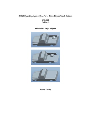
2. Purpose
In the United States, especially in Iowa, pickup trucks are a common vehicle with
very little research done on the aerodynamic drag on a truck. As prices of fuel increase
there is a growing awareness of fuel efficiency among the vehicles people drive. There is a
widely held belief that putting down the tailgate can decrease the drag and improve
efficiency. The airflow around trucks is more complicated than most because of the sharp
corners and large gap in the bed of the truck that is strictly for storage with no
consideration of aerodynamics. This project was created in order to observe the
differences between three different options that are available for the bed of a pickup truck:
lift gate up, down, and covered with a top.
Originally the model was tested trying to examine the effects of forces at a speed of
80 mph but was unable to obtain convergence with the limited mesh size and intricate
design of the pickup truck. A speed of 35 mph (15.64 m/s) was modeled at the inlet of a
fluid that runs over a car 180 inches (4.57 m) in length and 80 inches (2.032 m) in width.
The three cases were tested and the resulting flow around the pickup truck bed was
analyzed with pressure plots, velocity contour plots, vector velocity plots, and the resulting
forces and coefficients of drag that were obtained at convergence.
CFD Process
First, the truck geometry was constructed. Standard length, width, bed dimensions,
and other dimensions were researched online for existing trucks and a sketch was made to
replicate. Dimensions that were not found were based off of relative dimensions in Figure
1:

3. Figure 1 Pickup truck model used to dimension CAD drawing
The truck was modeled in PRO ENGINEERING with an overall length of 180 inches in length
and 80 inches in width. This model was then saved as an IGES solid file in order to import
the model into ANSYS geometry.
Once the model was imported and generated the fluid was then drawn with a half
car length of fluid flow in front and a full car length behind in order to allow for proper fluid
simulation. This was then Boolean subtracted in order to remove the model of the car from
the fluid and allow for proper flow. Since the model was created in PRO ENGINEER there
were multiple named selections that needed to be done in order to allow for ease of use in
ANSYS Fluent. The following surfaces were all highlighted and named as follows:
1. Truck surfaces – truck
2. Front of mesh – velocity-inlet

4. 3. Back of mesh – pressure-outlet
4. Bottom of mesh – road
5. Top of mesh – symmetry-top
6. Side of mesh –symmetry-side
Once these were all labeled an extra sketch was made closer to the truck in order to create
a finer mesh closer to the truck resulting in a final CFD mesh seen in Figure 2.
Figure 2 Model mesh used for representing the flow of air around a truck with lift gate up
Originally the model was created in ICEM CFD but was unable to appropriately mesh the
intricate geometry that was created properly. Multiple trials were done until research was
done on how to properly import PRO ENGINEERING files into ANSYS. This meshing
process was repeated for all three models with a final car mesh example shown in Figure 3
below.

5. Figure 3 Car mesh imported and check in ANSYS Fluent used to model airflow around
Multiple dimension changes and were done to the mesh in order to import into the solver
software Fluent because of the 512,000 element restriction on the student version.
The Physical settings of the examination were then entered into the Fluent software
in order to make sure the case was properly solved for. The Reynolds number was first
calculated to determine whether or not the flow was turbulent, which resulted in a
Reynolds number greater than 5 × 105
. This meant the k-epsilon viscous model was to be
utilized throughout the study to properly simulate the fluid flow around the truck. The
fluid was then defined as the default air and the default settings were correct. The
boundary conditions which had already been previously labeled in ANSYS Geometry were
also properly defined. A slight modification to inlet velocity specifying the component of x
velocity equal to 15.64 m/s which was 45 mph. The ANSYS software was then used to
calculate the projected surface on x of the truck, which was 1.45 m2
, this was entered into
the reference values along with selecting velocity-inlet as the reference.

6. A drag monitor was set up to plot on the screen and print in the command window
of Fluent to monitor when the result leveled out. This was a force vector set to be in the
positive x direction based off of the flow of fluid and geometry of the truck. The standard
initialization method was selected for this study with convergence criteria set to 1 × 106
.
After all settings for the model were double checked the solution method was first set to
SIMPLE and 400 iterations were ran for each model. A coupled solution method was then
set to solve for the solution for the next 400 iterations. Different modifications were done
to the model in order to converge the coefficient of drag for each model with results below
Figure 4 Coefficient of drag convergence for tailgate up design Figure 5 Coefficient of drag convergence for tailgate down design
Figure 6 Coefficient of drag convergence for covered design

7. As it can be seen in Figures 5 and 6 the solution converged much easier with the tailgate
down and a covered back design for the truck with very level results within 300 and 750
iterations. The coefficient of drag for the tailgate up design took over 2000 iterations for
the coefficient of drag to finally start to level off with multiple adjustments that were made
to each model.
It can be seen from the residuals that the intricate design for the truck provided many
different areas where the models for the different tailgates could not converge to a solution
easily. This in part can be due to the many curves that were modeled for the design and the
Figure 7 Residuals for the tailgate up design Figure 8 Residuals for the tailgate down design
Figure 9 Residuals for the covered design

8. amount surfaces that represented the truck designs. After hours of calculations the
coefficient of drags eventually were able to level off to a steady number for each model and
was considered stable enough for analysis.
Results
When representing the different truck models the main goal was to model the drag
seen be each design for the truck and understand where the different areas of drag occur
and for what reason. Analysis of the results efficiently and correctly was very important in
understanding why the drag for each design varied and where the largest magnitude
occurred. Overall the largest area of drag occurs with the overall shape of the object,
depending on the size and curves that went into each truck design. The main point of
interest for this study is the rear of the truck near the bed. Drag force in external flow
problems is the resultant force in the direction of upstream velocity. This force was the
only one of concern. The drag force is comprised of two parts, viscous and pressure
components. The viscous component of force is generated from the shear stress of the
fluid, in our case air, moving over the object. The pressure component of the force is the
normal stress of the fluid passing the object. This was first analyzed visually in Figure 10:

9. It can be observed above that the pressure magnitudes were largest near the front of the
truck from the pressure build near the stagnation point. There are slight pressure
variations near the back of each design so the drag force from pressure cannot be ignored
for these calculations. Velocity contour plots were then generated in order to analyze the
different velocity magnitudes that are observed as the flow of air moves over the truck and
towards the back truck bed.
Figure 10 Pressure distribution for tailgate up design
Figure 11 Pressure distribution for tailgate down design
Figure 12 Pressure distribution for covered design

10. The largest magnitudes of velocity took place near the very top of trucks and slowly
subsided from there. There is a large inflection in velocity magnitude from when the fluid
flows over the top of the truck to where somewhat stagnant are is located in the truck beds
for each design. The most amount of stagnant air appears to occur for the truck with the
tailgate down design represented by the darkest blue color observed. These observations
could not definitively say anything about the drag force that would be caused by the
different designs so further analysis of the back of each truck was done with a velocity
vector field shown in Figures 14-16:
Figure 13 Magnitude of velocity plots combined

11. These plots revealed the most interesting data for each of the flows. The tailgate up design
was iterated more in order to further analyze the result and revealed some interesting
features
Figure 17 Further analysis of velocity vector field in tailgate up design
Figure 14 Velocity vector for tailgate up design model Figure 15 Velocity vector for tailgate down design model
Figure 16 Velocity vector for a covered design model

12. Figure 17 really shows everything that is going on inside of the truck bed. There is a
circulation of stagnant air that continuously circulates over and over with only very little
that leaves the bed. This provides a sort of bubble that protects against a shear force on the
entire bed length, which would provide more drag on the truck. Further analysis into the
other two fields resulted in different results.
Figure 18 Further analysis of velocity vector field in order to understand shear stress on the covered design
Figure 19 Further analysis of velocity vector field in order to understand shear stress on the lift down design
Figures 18 and 19 reveal that there are velocity vector fields running parallel at larger
magnitude than with the lift gate up design. This will in turn contribute to the shear force
acting on the truck bed contribution to a larger drag force.

13. The resulting coefficient of drag for each model calculated in Fluent can be seen in
Table 1:
Table 1 Coefficient of drag calculated by Fluent solver
Coefficient of Drag
Design Fluent
Tailgate Up 0.3093
Tailgate Down 0.3523
Covered Back 0.3500
As expected the tailgate up design resulted in the lowest coefficient of drag because of the
stagnant air bubble that was produced from the swirling effect the tailgate provided on the
fluid flow. Using these numbers the theoretical force from drag was then also calculated
using Equation 1 below:
𝐹𝑑 = 𝐶 𝑑 𝐴𝜌
𝑉2
2
(1)
The resulting Fluent calculated and theoretical forces were then compared in Table 2
below:
Table 2 Drag force comparison of Ansys calculated to theoretical
Force of Drag [N]
Design Fluent Theoretical
Tailgate Up 132.89 136.20
Tailgate Down 142.78 146.45
Covered Back 148.60 152.06
These were very close to the theoretical calculated force of drag, which conforms with the
results that we have and what is expected.

14. Conclusion
The flow around a typical truck was simulated at 35 mph with designs where the
truck has its tailgate up, tailgate down, and a covered truck bed to understand which design
provided the least amount of drag and would be most fuel-efficient. The results concluded
that the most fuel-efficient setup for a truck was to drive with the tailgate up and
uncovered. This resulted in the least amount of drag force and a drag coefficient that was
almost 0.5 less than the other designs. Results from the simulations coincided with the
theoretical values for the drag force that the trucks would receive just slightly larger. From
the vector velocity fields of the different designs it could be stated that there are different
ways that the drag force for the tailgate down design and covered back. One option to
reduce the amount of drag would be to add a small device near the back of the truck beds
which would redirect the flow of air back towards the front of the truck created a similar
stagnant air pocket like in the lift gate up design. The truck design where an added taller
back that is flush with the cab was not modeled and compared to these different designs
but would be a very interesting addition to this study in order to better understand the
different drag forces on the truck. An initial guess would suggest that the drag force would
be large because of a larger amount of shear stress throughout the entire top of the truck
similar to a covered back design.

15. References
- Munson, Bruce Roy, Donald F. Young, and Theodore Hisao Okiishi. Fundamentals of
Fluid Mechanics. 7th ed. Hoboken, NJ: J. Wiley & Sons, 2006. Print.

16. Appendix
Figure 20 Vector velocity plots combined