This dataset contains information on accidental drug-related deaths in Connecticut from 2012 to June 2016. It includes details on the victim such as age, race, location of death, and specific drugs involved. The analysis found that areas with high death counts tend to have lower incomes and larger minority populations. For most races, heroin was the leading cause of death, but cocaine caused more deaths among black victims. While heroin remains a major problem, deaths related to fentanyl have grown rapidly in recent years. The highest death rates occur among adults ages 40-49, though most victims are between 20-60 years old. Addressing lack of education and employment opportunities in vulnerable communities could help curb the drug crisis.
This investigation analyzed the relationship between a country's GDP per capita and its male suicide rate per 100,000 people. Data on GDP and male suicide rates for 39 countries was collected from NationMaster.com and analyzed using statistical tests. A scatter plot, least squares regression, Pearson's correlation coefficient, and Chi-square test showed little to no correlation. The Chi-square test result supported the conclusion that male suicide rates and relative individual wealth of countries are independent factors. Limitations include potential inaccuracies in suicide rate data collected by some countries.
Statistics is the science of dealing with numbers and is used for collecting, summarizing, presenting, and analyzing data. It plays important roles in health care planning and evaluation, epidemiological studies, diagnosing community health problems, and comparing diseases and health status. Data can be quantitative or qualitative, discrete or continuous. Data is commonly presented using tables and graphs like bar charts, pie charts, histograms, scatter plots, and line graphs. Key measures used to summarize data include the mean, median, and mode for measures of central tendency, and the range, variance, and standard deviation for measures of dispersion.
Epidemiologists measure disease frequency and health status in populations using various metrics. Morbidity is measured using incidence rates which describe new cases over time. Incidence can be calculated as cumulative incidence from a stable population or incidence density using person-time. Mortality is measured using rates like crude death rate from the total population or age-adjusted rates to control for demographic factors. Rates express the probability of an event and are calculated by dividing the number of events by the population at risk over a specified time period.
This document analyzes potential excess death data from the United States from 2005 to 2015. It describes the datasets and variables, and performs various data refinements including removing missing values and misspelled text. Several visualizations and analyses are presented, examining trends in expected and observed deaths by year and age range, relationships between population and observed deaths by state, and social media discussions around different causes of death. Prediction models are developed to forecast future observed deaths based on variables like expected deaths, population, and region. A dashboard presents key findings visually.
1 LAB 3 INSTRUCTIONS ONE-SAMPLE AND TWO-SAMP.docxjoyjonna282
1
LAB 3 INSTRUCTIONS
ONE-SAMPLE AND TWO-SAMPLE INFERENCES
The primary purpose of the lab instructions is to demonstrate how the inferential tools in StatCrunch can be
applied to one-sample and two–sample problems about the mean and the difference in two population
means, respectively. In particular, you will learn how to obtain confidence intervals for the population
parameters of interest and how to test statistical hypotheses about the parameters. We will consider two
classes of inferential procedures available in StatCrunch depending on whether the population standard
deviation(s) are known or unknown.
1. One-Sample Inferences about the Mean
Statistical inference is inference about a population from a random sample drawn from it. We will
consider two important methods of statistical inference: interval estimation (confidence intervals)
and hypothesis testing (tests of significance).
(a) Confidence Intervals about the Mean
The purpose of a confidence interval is to estimate an unknown population parameter with an
indication of how accurate the estimate is and of how confident we are the result is correct. In
summary, a confidence interval contains the most plausible values for the parameter.
Any confidence interval has the form
Estimate of the parameter Margin of error.
A (1-α)∙100% confidence interval for the mean of a normal population with known standard
deviation , based on a random sample of size n, is given by
where se= / n is the standard error and / 2z is the z-score corresponding to the confidence
level 1-α. The z-score has right-tail probability α/2. In particular, z=1.96 when 1-α =0.95 (95%
confidence interval).
The confidence level C states the probability that the method will produce a confidence interval
containing the population parameter. That is, if you obtain 95% confidence intervals repeatedly, in
the long run 95% of your intervals will contain the true population parameter. However, you
cannot know whether a particular confidence interval contains the parameter.
When the population standard deviation σ is unknown, the standard error se is estimated by the
ratio /s n , where s is the sample standard deviation. In this case, the confidence interval is
based on the formula
where
/ 2
t
is the t-score of the t-distribution with (n-1) degrees of freedom and it has right tail
probability of α/2.
/ 2
( ),x z se
/ 2
( ),x t se
2
(b) Tests about the Mean
Another inferential method about the population mean μ called hypothesis testing analyzes the
evidence that the sample data provide in favor of a specific claim about the mean. In general, in
any hypothesis testing problem there are two alternative claims under consideration: the null
hypothesis denoted by H0 (the claim initially assumed to be true) and the alternative hypothesis
denoted by Ha (the claim we suspect is true instead of H0). Both h ...
The document analyzes the relationship between human birth rates and death rates in 18 countries. A scatter plot showed a strong negative correlation, indicating that higher birth rates were associated with lower death rates. Calculations for standard deviation, least squares regression, and Pearson's correlation coefficient supported this relationship. A chi-square test rejected independence, showing that birth and death rates were dependent. However, limitations included older data and lack of representation from all global regions. Overall, the analysis found an interdependent relationship between birth and death rates.
4. Performed statistical analysis on a chosen data table and understood relationship amongst different data fields using IBM SPSS software.
Methodologies: Multi linear regression, Logistic linear regression
IBM SPSS
The Judgement by Kafka Summary The leading character Geo.docxjmindy
This document summarizes key statistical concepts including descriptive statistics like measures of central tendency (mean, median, mode), measures of variability (range, variance, standard deviation), and measures of relationship. It provides examples to demonstrate how to calculate these statistics, such as calculating the mean, median, mode, range, sum of squares, variance and standard deviation for a sample dataset on truancy scores. It also discusses how regression analysis can be used to describe relationships between variables.
We are leading online solution provider for Statistics assignment.
Tutors here are excellent in data analysis using softwares like SPSS,
Stata ,Minitab, R, Excel, SAS, EViews etc. We also provide Statistic
assignment help for Time Series, Stochastics Problems and Linear
Programming. Email to info@statisticshelptutors.com for statistics
homework help.
The purpose of this document is to collect in a summarized way the main results of fire statistics recently published by different entities, both national and international.
Furthermore, an objective analysis of these results is performed and the most obvious conclusions are showed.
Cardiovascular epidemiology studies large patient databases and long-term followups to analyze risk factors for heart disease and sudden cardiac death. The unit conducts statistical analysis on clinical trial data and applies new approaches like data mining to generate insights. Most sudden cardiac deaths over age 35 are due to ischemic heart disease, while younger patients may experience conditions like hypertrophic cardiomyopathy.
An overview of a key statistical technique in epidemiology – standardization - is introduced. The process and application of both direct and indirect standardization in improving the validity of comparisons between populations are described.
This document analyzes the longitudinal medical costs of hypertensive diseases in Mexico from 2012 to 2050. It calculates probabilities of disease detection, treatment, and death by age and sex using historical Mexican health data. Medical costs are projected under base, optimal, and worse economic growth scenarios. Costs are higher for women and increase significantly after age 50. The maximum number of patients in treatment is between ages 20-29, decreasing until ages 65-69 for men and 60-64 for women before rising again with other age-related illnesses. Hypertensive disease costs are more expensive than diabetes and projected to increase as the population ages.
1. The document discusses several cases involving the use of demographic indices and statistical methods to analyze mortality data. These include calculating standardized mortality ratios to compare mortality rates between populations while adjusting for differences in age structure.
2. Indirect standardization is used in one case to compare the mortality of the Colombian department of Vichada to the overall mortality in Colombia using age-specific mortality rates.
3. Another case examines mortality trends among foundry workers using standardized mortality ratios and discusses methods to address potential biases from issues like loss to follow up.
Briefly describing:
(1.) Crude Death Rate
(2.) Specific Death Rate
(3.) Proportional Mortality Rate
(4.) Maternal Mortality Ratio (MMR)
(5.) Odds Ratio
(6.) Standardized Mortality Ratio (SMR)
(7.) Case Fatality Rate (CFR)
COVID-19 Update (Summary): September 28, 2020 Steve Shafer
This document provides context and sources for COVID-19 analyses and projections. It notes that the analyses are conducted independently of Stanford by an anesthesiologist to understand the trajectory of the pandemic. Models use a Gompertz function for case projections and log-linear regression for deaths. Locations are chosen based on the analyst's connections or significance. Data sources include Johns Hopkins, the COVID Tracking Project, and Oxford COVID-19 Government Response Tracker. Analyses aim to be apolitical while occasionally noting misrepresentations or risks from government policies.
COVID-19 Update (Summary): October 3, 2020 Steve Shafer
This document provides an overview and analysis of COVID-19 cases and projections worldwide and in several locations. It summarizes daily global and location-specific COVID-19 case and death numbers, and uses statistical modeling to project future case numbers. The document also explains data sources and modeling approaches, and provides figures with trend lines and projections for various geographies.
COVID-19 Update (Summary): October 9, 2020Steve Shafer
The document provides an overview and analysis of COVID-19 cases and projections globally and for several specific locations. It notes the data sources and modeling approaches used, and includes explanations of the various figures and metrics presented on the COVID-19 projections. The analysis is aimed at understanding the trajectory of the pandemic without political bias.
An empirical estimate of the infection fatality rate of COVID-19 from the fir...Guy Boulianne
1. The study estimates the infection fatality rate of COVID-19 in one of the hardest hit areas in Lombardy, Italy using demographic and death records data without relying on testing or death count data.
2. They estimate an overall infection fatality rate of 1.29% but find large differences by age, with a low rate of 0.05% for under 60 years old and a higher 4.25% for people over 60.
3. Sensitivity analysis found that even if only 10-15% of the population was infected, the fatality rate would still be below 1% for under 60s, showing COVID-19 has a low lethality for younger people but higher rates for older
PRIVATE AGE ADJUSTMENTWhen analyzing epidemiologic dat.docxsleeperharwell
PRIVATE
AGE ADJUSTMENT
When analyzing epidemiologic data, researchers often wish to adjust for the influence of some variable so that the "true" effect of other variables can be seen more clearly. Consider the example of a study to determine if gray hair is related to mortality risk. Two statements stand out in this study:
1. People with gray hair have a higher death rate when compared to other people.
2. People with gray hair are older than others people.
Because of this second statement the meaning of statement one is obscure. The possible link between gray hair and mortality risk is confused by the effect of age on mortality risk. Age is considered a confounding factor that needs to be accounted for to accurately assess the impact of gray hair on mortality rates. Epidemiologists use many tools to sort through information and overcome this confusion of information by adjusting data. The purpose of data adjustment is to disentangle the relationship so that we can evaluate a variables effect free from confusion and distortion. For the gray hair investigation, adjustment would permit us to determine whether persons of the same age who have gray hair have different mortality risks. (Sempos 1989)
Confounding Variables
Confounding variables are variables whose effects confuse the true relationships between factors and diseases. This is why there is a need for data adjustment. In order for a variable to be considered a confounding variable, it must be related to the disease or condition of interest and to the risk factor being investigated (Miettinen 1970). But if the possible confounding variable is truly related only to the disease of interest, it may still be desirable to adjust for it (Mantel 1986). One reason is the adjustment could possibly reduce the sampling variance of the comparison that is being investigated.
Adjustments
A common example of data adjustment is the age adjustment of mortality rates. While the age adjustment technique is most often applied to mortality (death) rates, it could also be applied to incidence of disease, prevalence, or any other kind of proportional rates. Age adjustment allows comparison of mortality risk for various groups free from the distortion of one group having a different age distribution than another. There are two types of age adjustments in relation to mortality rates -- direct and indirect age adjustments.
Direct Adjustment
Direct adjustment, or direct standardization, is to superimpose the age distribution of a standard population on the two study groups to be compared. Standardized rates are then calculated for each population, making use of the standard age distribution. These adjusted rates are then compared, and any difference between them can no longer be due to difference in age distribution because age has been taken into account. The direct method uses two inputs called age-specific rates and standard population.
Age-Specific Rates
A set of age-specif.
This document discusses a study examining the relationship between non-fatal motor vehicle collision (MVC) injuries, economic growth, and political governance. The study uses panel data from 64 countries between 1970 and 2009. Results show there is an inverted U-shaped relationship between income per capita and injury rate, consistent with the Kuznets curve. Additionally, factors like more vehicles per capita, urban population growth, and improvements in medical care were associated with lower injury rates. The study aims to better understand how economic and political factors impact road safety outcomes.
COVID-19 Update (Summary): October 6, 2020 Steve Shafer
The document provides an overview and analysis of COVID-19 cases and projections globally and in several locations. It notes the data sources and modeling approaches used, including Gompertz and log linear regression models. Charts and graphs displayed in the analysis provide daily case and death numbers, comparisons between locations, and rankings of countries. The analysis aims to be apolitical and provide daily updates on the COVID-19 trajectory.
COVID-19 Update (Summary): October 10, 2020Steve Shafer
The document provides context and explanations for COVID-19 projections and analyses. It notes that the analysis is conducted independently and aims to be apolitical. Data sources and modeling approaches are described, including using a Gompertz function to model case growth and log-linear regression for deaths. Locations are selected based on factors like family/friends or economic importance. Updates are typically daily, though clinical duties may cause delays.
This document summarizes a study examining variation in county-level stroke mortality rates in China between 1986-1988 and potential risk factors. The study found nearly a 7-fold difference in stroke mortality rates between counties for both men and women. Higher latitude was correlated with higher mortality. For women, higher blood pressure, green vegetable consumption, BMI, and HDL cholesterol were also correlated, but no single factor explained more than 20% of the variation. The study suggests stroke risk is influenced by combinations of multiple factors.
COVID-19 Update (Summary): September 27, 2020 Steve Shafer
This document provides context and explanations for COVID-19 projections and analyses. It notes that the analysis is conducted independently and aims to be apolitical. Data sources and modeling approaches are described, including using a Gompertz function to model case growth and log-linear regression for deaths. Locations are selected based on factors like family/friends or economic importance. Updates are typically daily, though clinical duties may cause delays.
COVID-19 Update (Summary): October 5, 2020 Steve Shafer
This document provides an overview and analysis of COVID-19 cases and projections globally and in several locations. It summarizes models and data sources used in the analysis and projections. Updates are typically provided daily, with this report on October 5th finding over 35 million global cases and over 1 million deaths, with the US reporting over 7.4 million cases and over 209,000 deaths.
[M3A2] Data Analysis and Interpretation Specialization Andrea Rubio
The document discusses testing a linear regression model to analyze the relationship between the number of terrorists participating in an incident (explanatory variable) and the total number of fatalities (response variable) using data from the Global Terrorism Database. Code is presented that imports data, converts variables to numeric, and runs an OLS regression. The results show a statistically significant positive association between the number of terrorists and fatalities. A codebook defining and explaining the variables is also included.
COVID-19 Update (Summary): October 8, 2020 Steve Shafer
This document provides context and explanations for COVID-19 analyses and projections. It notes that the analyses are conducted independently and aim to be apolitical. Data sources and modeling approaches are described, including using a Gompertz function to model cumulative cases and log-linear regression for deaths. Locations are selected based on factors like family/friends or economic impact. Updates are typically daily, though clinical duties may cause delays.
More Related Content
Similar to Analysis of drug related deaths in state of Connecticut
We are leading online solution provider for Statistics assignment.
Tutors here are excellent in data analysis using softwares like SPSS,
Stata ,Minitab, R, Excel, SAS, EViews etc. We also provide Statistic
assignment help for Time Series, Stochastics Problems and Linear
Programming. Email to info@statisticshelptutors.com for statistics
homework help.
The purpose of this document is to collect in a summarized way the main results of fire statistics recently published by different entities, both national and international.
Furthermore, an objective analysis of these results is performed and the most obvious conclusions are showed.
Cardiovascular epidemiology studies large patient databases and long-term followups to analyze risk factors for heart disease and sudden cardiac death. The unit conducts statistical analysis on clinical trial data and applies new approaches like data mining to generate insights. Most sudden cardiac deaths over age 35 are due to ischemic heart disease, while younger patients may experience conditions like hypertrophic cardiomyopathy.
An overview of a key statistical technique in epidemiology – standardization - is introduced. The process and application of both direct and indirect standardization in improving the validity of comparisons between populations are described.
This document analyzes the longitudinal medical costs of hypertensive diseases in Mexico from 2012 to 2050. It calculates probabilities of disease detection, treatment, and death by age and sex using historical Mexican health data. Medical costs are projected under base, optimal, and worse economic growth scenarios. Costs are higher for women and increase significantly after age 50. The maximum number of patients in treatment is between ages 20-29, decreasing until ages 65-69 for men and 60-64 for women before rising again with other age-related illnesses. Hypertensive disease costs are more expensive than diabetes and projected to increase as the population ages.
1. The document discusses several cases involving the use of demographic indices and statistical methods to analyze mortality data. These include calculating standardized mortality ratios to compare mortality rates between populations while adjusting for differences in age structure.
2. Indirect standardization is used in one case to compare the mortality of the Colombian department of Vichada to the overall mortality in Colombia using age-specific mortality rates.
3. Another case examines mortality trends among foundry workers using standardized mortality ratios and discusses methods to address potential biases from issues like loss to follow up.
Briefly describing:
(1.) Crude Death Rate
(2.) Specific Death Rate
(3.) Proportional Mortality Rate
(4.) Maternal Mortality Ratio (MMR)
(5.) Odds Ratio
(6.) Standardized Mortality Ratio (SMR)
(7.) Case Fatality Rate (CFR)
COVID-19 Update (Summary): September 28, 2020 Steve Shafer
This document provides context and sources for COVID-19 analyses and projections. It notes that the analyses are conducted independently of Stanford by an anesthesiologist to understand the trajectory of the pandemic. Models use a Gompertz function for case projections and log-linear regression for deaths. Locations are chosen based on the analyst's connections or significance. Data sources include Johns Hopkins, the COVID Tracking Project, and Oxford COVID-19 Government Response Tracker. Analyses aim to be apolitical while occasionally noting misrepresentations or risks from government policies.
COVID-19 Update (Summary): October 3, 2020 Steve Shafer
This document provides an overview and analysis of COVID-19 cases and projections worldwide and in several locations. It summarizes daily global and location-specific COVID-19 case and death numbers, and uses statistical modeling to project future case numbers. The document also explains data sources and modeling approaches, and provides figures with trend lines and projections for various geographies.
COVID-19 Update (Summary): October 9, 2020Steve Shafer
The document provides an overview and analysis of COVID-19 cases and projections globally and for several specific locations. It notes the data sources and modeling approaches used, and includes explanations of the various figures and metrics presented on the COVID-19 projections. The analysis is aimed at understanding the trajectory of the pandemic without political bias.
An empirical estimate of the infection fatality rate of COVID-19 from the fir...Guy Boulianne
1. The study estimates the infection fatality rate of COVID-19 in one of the hardest hit areas in Lombardy, Italy using demographic and death records data without relying on testing or death count data.
2. They estimate an overall infection fatality rate of 1.29% but find large differences by age, with a low rate of 0.05% for under 60 years old and a higher 4.25% for people over 60.
3. Sensitivity analysis found that even if only 10-15% of the population was infected, the fatality rate would still be below 1% for under 60s, showing COVID-19 has a low lethality for younger people but higher rates for older
PRIVATE AGE ADJUSTMENTWhen analyzing epidemiologic dat.docxsleeperharwell
PRIVATE
AGE ADJUSTMENT
When analyzing epidemiologic data, researchers often wish to adjust for the influence of some variable so that the "true" effect of other variables can be seen more clearly. Consider the example of a study to determine if gray hair is related to mortality risk. Two statements stand out in this study:
1. People with gray hair have a higher death rate when compared to other people.
2. People with gray hair are older than others people.
Because of this second statement the meaning of statement one is obscure. The possible link between gray hair and mortality risk is confused by the effect of age on mortality risk. Age is considered a confounding factor that needs to be accounted for to accurately assess the impact of gray hair on mortality rates. Epidemiologists use many tools to sort through information and overcome this confusion of information by adjusting data. The purpose of data adjustment is to disentangle the relationship so that we can evaluate a variables effect free from confusion and distortion. For the gray hair investigation, adjustment would permit us to determine whether persons of the same age who have gray hair have different mortality risks. (Sempos 1989)
Confounding Variables
Confounding variables are variables whose effects confuse the true relationships between factors and diseases. This is why there is a need for data adjustment. In order for a variable to be considered a confounding variable, it must be related to the disease or condition of interest and to the risk factor being investigated (Miettinen 1970). But if the possible confounding variable is truly related only to the disease of interest, it may still be desirable to adjust for it (Mantel 1986). One reason is the adjustment could possibly reduce the sampling variance of the comparison that is being investigated.
Adjustments
A common example of data adjustment is the age adjustment of mortality rates. While the age adjustment technique is most often applied to mortality (death) rates, it could also be applied to incidence of disease, prevalence, or any other kind of proportional rates. Age adjustment allows comparison of mortality risk for various groups free from the distortion of one group having a different age distribution than another. There are two types of age adjustments in relation to mortality rates -- direct and indirect age adjustments.
Direct Adjustment
Direct adjustment, or direct standardization, is to superimpose the age distribution of a standard population on the two study groups to be compared. Standardized rates are then calculated for each population, making use of the standard age distribution. These adjusted rates are then compared, and any difference between them can no longer be due to difference in age distribution because age has been taken into account. The direct method uses two inputs called age-specific rates and standard population.
Age-Specific Rates
A set of age-specif.
This document discusses a study examining the relationship between non-fatal motor vehicle collision (MVC) injuries, economic growth, and political governance. The study uses panel data from 64 countries between 1970 and 2009. Results show there is an inverted U-shaped relationship between income per capita and injury rate, consistent with the Kuznets curve. Additionally, factors like more vehicles per capita, urban population growth, and improvements in medical care were associated with lower injury rates. The study aims to better understand how economic and political factors impact road safety outcomes.
COVID-19 Update (Summary): October 6, 2020 Steve Shafer
The document provides an overview and analysis of COVID-19 cases and projections globally and in several locations. It notes the data sources and modeling approaches used, including Gompertz and log linear regression models. Charts and graphs displayed in the analysis provide daily case and death numbers, comparisons between locations, and rankings of countries. The analysis aims to be apolitical and provide daily updates on the COVID-19 trajectory.
COVID-19 Update (Summary): October 10, 2020Steve Shafer
The document provides context and explanations for COVID-19 projections and analyses. It notes that the analysis is conducted independently and aims to be apolitical. Data sources and modeling approaches are described, including using a Gompertz function to model case growth and log-linear regression for deaths. Locations are selected based on factors like family/friends or economic importance. Updates are typically daily, though clinical duties may cause delays.
This document summarizes a study examining variation in county-level stroke mortality rates in China between 1986-1988 and potential risk factors. The study found nearly a 7-fold difference in stroke mortality rates between counties for both men and women. Higher latitude was correlated with higher mortality. For women, higher blood pressure, green vegetable consumption, BMI, and HDL cholesterol were also correlated, but no single factor explained more than 20% of the variation. The study suggests stroke risk is influenced by combinations of multiple factors.
COVID-19 Update (Summary): September 27, 2020 Steve Shafer
This document provides context and explanations for COVID-19 projections and analyses. It notes that the analysis is conducted independently and aims to be apolitical. Data sources and modeling approaches are described, including using a Gompertz function to model case growth and log-linear regression for deaths. Locations are selected based on factors like family/friends or economic importance. Updates are typically daily, though clinical duties may cause delays.
COVID-19 Update (Summary): October 5, 2020 Steve Shafer
This document provides an overview and analysis of COVID-19 cases and projections globally and in several locations. It summarizes models and data sources used in the analysis and projections. Updates are typically provided daily, with this report on October 5th finding over 35 million global cases and over 1 million deaths, with the US reporting over 7.4 million cases and over 209,000 deaths.
[M3A2] Data Analysis and Interpretation Specialization Andrea Rubio
The document discusses testing a linear regression model to analyze the relationship between the number of terrorists participating in an incident (explanatory variable) and the total number of fatalities (response variable) using data from the Global Terrorism Database. Code is presented that imports data, converts variables to numeric, and runs an OLS regression. The results show a statistically significant positive association between the number of terrorists and fatalities. A codebook defining and explaining the variables is also included.
COVID-19 Update (Summary): October 8, 2020 Steve Shafer
This document provides context and explanations for COVID-19 analyses and projections. It notes that the analyses are conducted independently and aim to be apolitical. Data sources and modeling approaches are described, including using a Gompertz function to model cumulative cases and log-linear regression for deaths. Locations are selected based on factors like family/friends or economic impact. Updates are typically daily, though clinical duties may cause delays.
Similar to Analysis of drug related deaths in state of Connecticut (20)
Analysis of drug related deaths in state of Connecticut
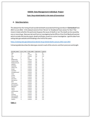
1. IS6030: Data Management-Individual Project
Topic: Drug related deaths in the state of Conncecticut
A. Data Description:
Thisdatasethas the listingof eachaccidental deathassociatedwithdrugoverdosein Connecticutfrom
2012 to June 2016. Inthisdatasetcolumnsfrom‘Heroin’to‘AnyOpioid’have valuesYor Null.That
meansitstateswhetherthe particulardrugwas the cause of deathor not.The deathcan be causedby
one or more drugs. Data was derivedfromaninvestigationbythe Office of the Chief Medical Examiner
whichincludesthe toxicityreport,deathcertificate,aswell asa scene investigation. Igotthisdata from
catlog.data.govwebsite andfollowingisthe linkforthe same:
https://catalog.data.gov/dataset/accidental-drug-related-deaths-january-2012-sept-2015
Followingtabledescribesthe datatypesstoredineachof the columns and theirprecisionandlength:
Table: 1
2. Afterimportingthe datasetinSQLserver,Imade sure that all data typesare appropriate anddata is
importedcorrectly.(Code forthe same isincludedincode file).Inthe nextstepIdidsome basicchecks
on importantcolumnslike findingoutdistinct values,numberof null recordsandmaximum, minimum
and average valuesforthe numerical variablesetc.:
Sex:
Race:
Death cause:
Death locations:
Thisdata can be normalizedusing‘Case Number’asthe primarykey(Thiscolumnwasremovedfrom
datasetas it wasnot necessaryforanalysis).Andthe othercolumnslike age,race,‘ImmeddiatecauseA’
etc.can be put intodifferenttable withforeignkeyinthe maintable.
B. Data Issues:
There were manydata issuesthatneededtobe resolvedbeforestartingthe analysisonthe data:
1. Null Values:There were some null valuesinsome columnsof the dataset.Asthe numberwas
not verylarge (max:7) these recordswere removedfromthe dataset. Thiswasdone inexcel.
2. Date Format: While importingdatasetinTableu,Ifoundthatdate format is not consistent.(Idid
not face thisissue inwhile importingdatainSQL).To solve thisIcreatedtwomore columnsfor
yearand month.(Before doingthissome yearvaluesweremissingfromthe visualizationdue to
improperformat)
3. Data structure: With the currentdata structure it wasnot possible togetrequiredvisualizations
inTableu.Data was restructuredinexcel togetthe same.
4. Inconsistencyin time frame: Inorder to compare the data across the years,average death
count permonthwas usedas foryear 2016, data of onlysix monthsisavailable.
Most of these operationsweredone inusingExcel.Alsofunctionslike‘SUMIFS’,‘CONCAT’,
‘RIGHT’, ‘MID’,‘YEAR()’,‘MONTH()’etc.were used.
3. C. Data Analysis in SQL:
Total Numberof rows:
Total numberof columns:
Numberof deathsbyyear: (countfor2016 will be lessasit has onlysix monthsdata):
Numberof deathsbySex:
Numberof deathsbyage bracket:
Max, minand average valuesforage:
4. Numberof deathsbyRace:
D. Primary Data Analysis using Tableau :
Average deathcountpermonthis increasingwithalmostconstantrate overpast5 years:
Fig. 1
5. From Figures2,3 and 4, we can see thatthoughthe numberof average deathspermonthis maximum
for White people,areaswith maximumnumberof deaths (countof all deathsfrom2012-2016) are
mainly concentratednearthe locationswherepopulationof Black,HispanicandLatinopeople isdense:
Fig. 2
Fig. 3
6. Fig. 4
For all the races exceptBlackHeroinwasthe leading cause of death,butincase of blacks Cocaine was
the leadingcause:
Fig. 5
7. Numberof average deathspermonth ismaximumforage group of 40-49 and inall age group20-60 is
the primary victim:
Fig. 6
Heroinisthe main cause of deathsfollowedby cocaine:
Fig. 7
8. Comparedtoall otherdrugsFentanyl hasthe highestincrease inthe deathsoverthe years.Aswe can
see fromthe figure below,deathcount because of all otherdrugsincreasessteadily,butthere isajump
inthe numberof deathsbecause of Fentanyl (speciallyin2016):
Fig. 8
From the following plot, we canclearlysee thatareaswithmaximumnumberof deathsare
concentratedexactlynearthe locationswherepercapitaincome isquite low:
Fig. 9
9. Followingisthe graphof Age vstotal numberof deathsfromyear2012-2016. From the thisgraph we
can see that there isa strong positive correlationbetweenage andnumberof deathsinthe lower
spectrumof age and a strongnegative correlationinhigherspectrumof age.
Fig. 10
E. Correlation and Regression Analysis using R-studio:
Let’scheck the correlationandrunthe regressionanalysisonthe same:
R-studiowasusedtorun the statistical analysisonthe data.
a. CorrelationAnalysis:
1. Followingisthe correlationbetweenage (lowerage group15-25) and the average numberof
deathsperyear (i.e.Total numberof deaths/4.5,astotal numberof yearsis 4.5):
0.9812866
2. Followingisthe correlationbetweenage (Middle age group26-44) and the average numberof
deathsperyear:
0.1022106
3. Followingisthe correlationbetweenage (higherage group45-80) and the average numberof
deathsperyear:
-0.955015
10. b. RegressionAnalysis:
As we can see fromabove valuesthere ishighcorrelationin lowerandhigherrange of agesand
the average numberof deathsperyear. Now we will runthe regressionanalysis (UsingR-studio)
on these age groups:
1. Regressionanalysison Lower Age group (15-25):
Followingisthe plotof the lowerage groupvsaverage numberof deathsperyear:
Fig. 11
Let’srun the regressionmodel onthe data:
11. From the above outputwe can see that ‘P’valuesforbothage and interceptare lessthan0.05. This
meansthat ‘Beta’coefficientforage issignificantlydifferentfrom 0 andage issignificantfactorinthe
regressionmodel. Asthisissimple linearregressionmodel we getthe same Pvaluesfort-testandF-
test.
Alsothe valuesforR-square andadjustedR-square are quite highi.e.0.9629 and 0.9583 respectively.
So, the final model thatwe generate fromabove analysis:
Average number of deathsper year=1.7576*(Age) - 28.1160
Let ustake a lookat the plotof residualsvsfittedvalues:
s
Fig. 12
As we can see fromthe above plotthere isno specificpatterninthe residuals,theyare randomly
scattered. Thismeansthatwe have capturedmost of the signal fromthe data indeterministicpartof
our model andremainingisjustarandom noise.
12. Now,let’scheck the normalityof the residuals usingthe q-qplot.Thisisourassumptionandwe needto
validate that:
Fig. 13
We can clearlysee thatabove q-qplotisprettymuch a straightline passingthrough0 whichvalidates
our assumptionof normalityof errors withmean0 (asline ispassingthrough0).
13. 2. Regressionanalysison Higher Age group (45-80):
Followingisthe plotof the higherage groupvsaverage numberof deathsperyear:
Fig. 14
Now,let’srunthe regressionmodel onthe data:
14. From the above outputwe can see that ‘P’valuesforbothage and interceptare lessthan0.05 for
higherage groupas well.Thismeansthat‘Beta’coefficientforage issignificantlydifferentfrom0and
age issignificantfactorinthe regressionmodel. As thisissimple linearregressionmodelwe getthe
same P valuesfort-testandF-test.
Alsothe valuesforR-square andadjustedR-square are quite highi.e.0.9121 and 0.9089 respectively.
So,the final model thatwe generate fromabove analysis:
Average number of deathsper year=(-0.91072)*(Age) +65.06579
Let ustake a lookat the plotof residualsvsfittedvalues:
Fig. 15
As we can see fromthe above plot there isa straightline of residualsinthe lowerregionof fittedvalues,
but onoverall level itlooksquite scattered. Thismeansthatwe have capturedmostof the signal from
the data (specificallyinhigherfittedvalue spectrum) indeterministicpartof our model andremainingis
justa randomnoise.
15. Now,let’scheckthe normalityof the residuals usingthe q-qplot.Thisisourassumptionandwe needto
validate that:
Fig. 16
We can see fromabove plotthat apart fromthe curvature at the (-1) quantile,ourplotismostlya
straightline.
16. F. Key Findings and Insights:
1. The areas withmaximumnumberof deathsare concentratedexactlynearthe locationswhere
percapita income isquite low
2. The areas withmaximumnumberof deathsare mainlyconcentratednearthe locationswhere
populationof Black,HispanicandLatinopeople is dense thoughtthe numberof deathsbydrug
are maximumforwhite people
3. For all the races exceptBlack, Heroinwasthe leadingcause of death,butincase of blacksit was
Cocaine
4. ThoughHeroinisthe maincause,Fentanyl hasthe highest rate of increase inthe deaths count
overthe years.
5. Numberof average deathspermonthismaximumforage group of 40-49
6. We couldsee the peaksinthe deathcount aroundage 30 andage 50 and there isa dipin the
deathcount aroundage 40.
G. Suggestions:
1. As we clearly see thatage group 20-60, whichisthe backbone generationof anynation, isthe
primaryvictimof the drugs and thatis mainlydue tolow income whichinturnI thinkisdue to
lack of education(whichcanprovide themwithdecentjobs).Thisisthe bigconcern as number
isincreasingeveryyearandgovernmentneedstoaddressthisissue andplantoprovide basic
educationtothese people whichcanmake thememployable.
2. As Fentanyl hasthe highestgrowthinthe drugcount,it isnot enoughtocurb the supplyof just
heroinorcocaine
H. Challenges:
1. Many data issuesneededtobe resolvedwhile plottingdatainTableau.Learnedvarious
functionsinexcel toovercome them.
2. As there were toomanyvariablesinthe data,itwas difficulttocarryout the structured
exploratorydataanalysistogainmeaningfulinsights.Example,variableslike age,race,typesof
drugsetc. formnumerousnumberof combinationsonwhichthe trendof deathcountcouldbe
analyzed.