Advanced data structure concepts

1. CS200: Algorithm Analysis
Mathematical Foundations for this class
are found in book appendices - begin
reviewing Appendix A.

2. Introduction to Algorithms - CH1
What is an algorithm?
•A well-defined general computational
process that takes a set of values as input
and produces a set of values as output,
{process is finite, output is correct}.
•A function that maps an input instance to a
correct output instance and halts, f(a) = b.

3. What is algorithm analysis?
•Application of mathematical
techniques to determine the relative
efficiency of an algorithm
Why analyze algorithms?
•Programmer maturity
•Select the best algorithm for the job
•Identify intractable problems (NP-
complete)
•Computers are not infinitely fast nor is
memory unlimited

4. Example: Two Fibonacci algorithms,
which is more efficient and why?
How to measure efficiency? What
efficiency metric should be used? How is
the metric quantified?
•Recursive algorithm is elegant but time efficiency is
exponential in n, space efficiency is linear in n -
repeated sub-problems (more later)
•Loop algorithm has a linear time efficiency in n and
uses a constant amount of space - a simple dynamic
programming algorithm (more later)
•Recursion is still a powerful tool

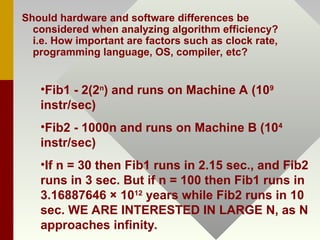
5. Should hardware and software differences be
considered when analyzing algorithm efficiency?
i.e. How important are factors such as clock rate,
programming language, OS, compiler, etc?
•Fib1 - 2(2n
) and runs on Machine A (109
instr/sec)
•Fib2 - 1000n and runs on Machine B (104
instr/sec)
•If n = 30 then Fib1 runs in 2.15 sec., and Fib2
runs in 3 sec. But if n = 100 then Fib1 runs in
3.16887646 × 1012
years while Fib2 runs in 10
sec. WE ARE INTERESTED IN LARGE N, as N
approaches infinity.

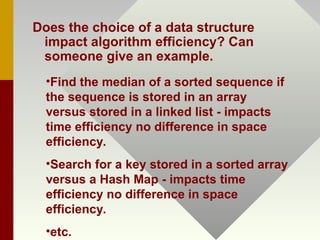
6. Does the choice of a data structure
impact algorithm efficiency? Can
someone give an example.
•Find the median of a sorted sequence if
the sequence is stored in an array
versus stored in a linked list - impacts
time efficiency no difference in space
efficiency.
•Search for a key stored in a sorted array
versus a Hash Map - impacts time
efficiency no difference in space
efficiency.
•etc.

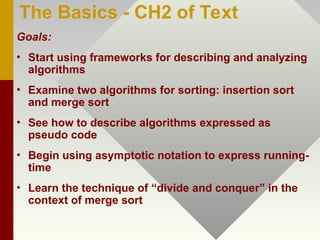
7. The Basics - CH2 of Text
Goals:
• Start using frameworks for describing and analyzing
algorithms
• Examine two algorithms for sorting: insertion sort
and merge sort
• See how to describe algorithms expressed as
pseudo code
• Begin using asymptotic notation to express running-
time
• Learn the technique of “divide and conquer” in the
context of merge sort

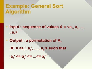
8. Example: General Sort
Algorithm
• Input : sequence of values A = <a1, a2, ...
, an>
• Output : a permutation of A,
A' = <a1', a2', ... , an'> such that
a1' <= a2' <= ...<= an'

9. Insertion Sort Pseudo Code Example
InsertionSort(A)
1. for j = 2 to n do
2. key = A[j]
4. i = j – 1
5. while(i>0)and(A[i]>key) do
6. A[i+1] = A[i]
7. i = i -1
8. A[i + 1] = key
A good algorithm for sorting a small number of
elements.
It works the way you might sort a hand of playing
cards.

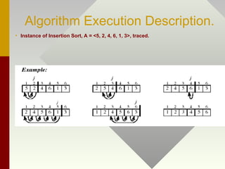
10. Algorithm Execution Description.
• Instance of Insertion Sort, A = <5, 2, 4, 6, 1, 3>, traced.
• Animation - https://en.wikipedia.org/wiki/Insertion_sort

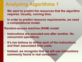
11. Analyzing Algorithms 1
• We want to predict the resources that the algorithm
requires. Usually, running time.
• In order to predict resource requirements, we need
a computational model.
Random-access machine (RAM) model
• Instructions are executed one after another. No
concurrent operations.
• It’s too tedious to define each of the instructions
and their associated time costs.
• Instead, we recognize that we will use instructions
commonly found in real computers:

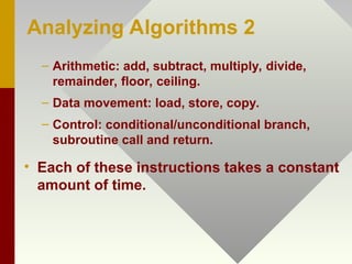
12. Analyzing Algorithms 2
– Arithmetic: add, subtract, multiply, divide,
remainder, floor, ceiling.
– Data movement: load, store, copy.
– Control: conditional/unconditional branch,
subroutine call and return.
• Each of these instructions takes a constant
amount of time.

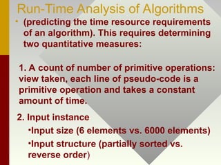
13. Run-Time Analysis of Algorithms
• (predicting the time resource requirements
of an algorithm). This requires determining
two quantitative measures:
1. A count of number of primitive operations:
view taken, each line of pseudo-code is a
primitive operation and takes a constant
amount of time.
2. Input instance
•Input size (6 elements vs. 6000 elements)
•Input structure (partially sorted vs.
reverse order)

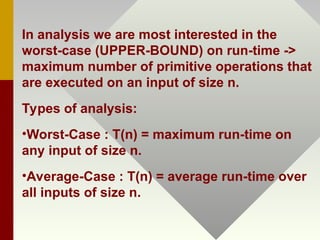
14. In analysis we are most interested in the
worst-case (UPPER-BOUND) on run-time ->
maximum number of primitive operations that
are executed on an input of size n.
Types of analysis:
•Worst-Case : T(n) = maximum run-time on
any input of size n.
•Average-Case : T(n) = average run-time over
all inputs of size n.

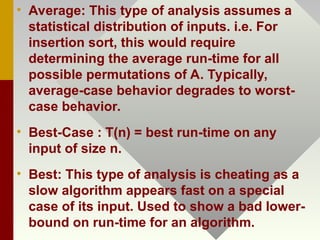
15. • Average: This type of analysis assumes a
statistical distribution of inputs. i.e. For
insertion sort, this would require
determining the average run-time for all
possible permutations of A. Typically,
average-case behavior degrades to worst-
case behavior.
• Best-Case : T(n) = best run-time on any
input of size n.
• Best: This type of analysis is cheating as a
slow algorithm appears fast on a special
case of its input. Used to show a bad lower-
bound on run-time for an algorithm.

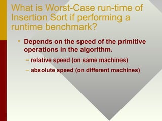
16. What is Worst-Case run-time of
Insertion Sort if performing a
runtime benchmark?
• Depends on the speed of the primitive
operations in the algorithm.
– relative speed (on same machines)
– absolute speed (on different machines)

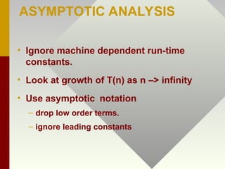
17. ASYMPTOTIC ANALYSIS
• Ignore machine dependent run-time
constants.
• Look at growth of T(n) as n –> infinity
• Use asymptoticnotation
– drop low order terms.
– ignore leading constants

18. Formal Application of Asymptotic
Notation
Insertion Sort Analysis
Cost Times
1. for j = 2 to n do c1 n
2. key = A[j] c2 n-1
4. i = j -1 c4 n-1
5. while(i>0) and (A[i]>key) do
c5  (tj)
6. A[i+1] = A[i] c6 (tj-1)
7. i = i -1 c7 (tj-1)
8. A[i+1] = key c8 n-1

19. Collecting Terms (proof)
T(n)=c1n+c2(n-1)+c4(n-1)+c5( tj)+c6([ tj-1])+
c7( [tj-1])+c8(n-1) bound on each summation is j = 2 … n
• Worst-case occurs when array is in reverse sorted
order: tj = j for j = 2, 3, ... , n because each A[j] must be
compared to each element in the sorted sub-array.
• Simplify T(n) by finding closed form for summations
and gathering terms.
• T(n) = an2
+bn + c = (n2
) Worst Case

20. • Average-case run time for insertion sort
occurs when all permutations of elements
are equally likely: tj = j/2 because on
average half of the elements in A[1..j-1] are
< A[j] and half are > A[j].
• Simplify T(n) by finding closed form for
summations and gathering terms.
• T(n) = an2
+bn + c = (n2
) Average Case

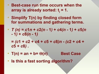
21. • Best-case run time occurs when the
array is already sorted: tj = 1.
• Simplify T(n) by finding closed form
for summations and gathering terms.
• T (n) = c1n + c2(n - 1) + c4(n - 1) + c5(n
- 1) + c8(n - 1)
= (c1 + c2 + c4 + c5 + c8)n - (c2 + c4 +
c5 + c8) .
• T(n) = an + b= (n) Best Case
• Is this a fast sorting algorithm?

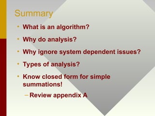
22. Summary
• What is an algorithm?
• Why do analysis?
• Why ignore system dependent issues?
• Types of analysis?
• Know closed form for simple
summations!
– Review appendix A