R cheat sheet

1. Advanced R
Cheat Sheet
Environment Basics
RStudio® is a trademark of RStudio, Inc. • CC BY Arianne Colton, Sean Chen • data.scientist.info@gmail.com • 844-448-1212 • rstudio.com Updated: 2/16
Environments
Environment – Data structure (with two
components below) that powers lexical scoping
1. Named list (“Bag of names”) – each name
points to an object stored elsewhere in
memory.
If an object has no names pointing to it, it
gets automatically deleted by the garbage
collector.
• Access with: ls('env1')
2. Parent environment – used to implement
lexical scoping. If a name is not found in
an environment, then R will look in its
parent (and so on).
• Access with: parent.env('env1')
Four special environments
1. Empty environment – ultimate ancestor of
all environments
• Parent: none
• Access with: emptyenv()
2. Base environment - environment of the
base package
• Parent: empty environment
• Access with: baseenv()
3. Global environment – the interactive
workspace that you normally work in
• Parent: environment of last attached
package
• Access with: globalenv()
4. Current environment – environment that
R is currently working in (may be any of the
above and others)
• Parent: empty environment
• Access with: environment()
1. Enclosing environment - an environment where the
function is created. It determines how function finds
value.
• Enclosing environment never changes, even if the
function is moved to a different environment.
• Access with: environment(‘func1’)
2. Binding environment - all environments that the
function has a binding to. It determines how we find
the function.
• Access with: pryr::where(‘func1’)
Example (for enclosing and binding environment):
3. Execution environment - new created environments
to host a function call execution.
• Two parents :
I. Enclosing environment of the function
II. Calling environment of the function
• Execution environment is thrown away once the
function has completed.
4. Calling environment - environments where the
function was called.
• Access with: parent.frame(‘func1’)
• Dynamic scoping :
• About : look up variables in the calling
environment rather than in the enclosing
environment
• Usage : most useful for developing functions that
aid interactive data analysis
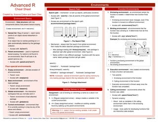
Function Environments
Search path – mechanism to look up objects, particularly functions.
• Access with : search() – lists all parents of the global environment
(see Figure 1)
• Access any environment on the search path:
as.environment('package:base')
Figure 1 – The Search Path
• Mechanism : always start the search from global environment,
then inside the latest attached package environment.
• New package loading with library()/require() : new package is
attached right after global environment. (See Figure 2)
• Name conflict in two different package : functions with the same
name, latest package function will get called.
Figure 2 – Package Attachment
search() :
'.GlobalEnv' ... 'Autoloads' 'package:base'
library(reshape2); search()
'.GlobalEnv' 'package:reshape2' ... 'Autoloads' 'package:base‘
NOTE: Autoloads : special environment used for saving memory by
only loading package objects (like big datasets) when needed
Search Path
Binding Names to Values
Assignment – act of binding (or rebinding) a name to a value in an
environment.
1. <- (Regular assignment arrow) – always creates a variable in the
current environment
2. <<- (Deep assignment arrow) - modifies an existing variable
found by walking up the parent environments
Warning: If <<- doesn’t find an existing variable, it will create
one in the global environment.
y <- 1
e <- new.env()
e$g <- function(x) x + y
• function g enclosing environment is the global
environment,
• the binding environment is "e".
Create environment: env1<-new.env()
Created by: Arianne Colton and Sean Chen

2. Human readable description of any R data structure :
Every Object has a mode and a class
1. Mode: represents how an object is stored in memory
• ‘type’ of the object from R’s point of view
• Access with: typeof()
2. Class: represents the object’s abstract type
• ‘type’ of the object from R’s object-oriented programming
point of view
• Access with: class()
RStudio® is a trademark of RStudio, Inc. • CC BY Arianne Colton, Sean Chen • data.scientist.info@gmail.com • 844-448-1212 • rstudio.com Updated: 2/16
Data Structures
1. Factors are built on top of integer vectors using two attributes :
2. Useful when you know the possible values a variable may take,
even if you don’t see all values in a given dataset. Base Type (C Structure)
S3
R has three object oriented systems :
1. S3 is a very casual system. It has no formal
definition of classes. It implements generic
function OO.
• Generic-function OO - a special type of
function called a generic function decides
which method to call.
• Message-passing OO - messages
(methods) are sent to objects and the object
determines which function to call.
2. S4 works similarly to S3, but is more formal.
Two major differences to S3 :
• Formal class definitions - describe the
representation and inheritance for each class,
and has special helper functions for defining
generics and methods.
• Multiple dispatch - generic functions can
pick methods based on the class of any
number of arguments, not just one.
3. Reference classes are very different from S3
and S4:
• Implements message-passing OO -
methods belong to classes, not functions.
• Notation - $ is used to separate objects and
methods, so method calls look like
canvas$drawRect('blue').
1. About S3 :
• R's first and simplest OO system
• Only OO system used in the base and stats
package
• Methods belong to functions, not to objects or
classes.
2. Notation :
• generic.class()
3. Useful ‘Generic’ Operations
• Get all methods that belong to the ‘mean’
generic:
- Methods(‘mean’)
• List all generics that have a method for the
‘Date’ class :
- methods(class = ‘Date’)
4. S3 objects are usually built on top of lists, or
atomic vectors with attributes.
• Factor and data frame are S3 class
• Useful operations:
Object Oriented (OO) Field Guide
mean.Date()
Date method for the
generic - mean()
Example: drawRect(canvas, 'blue')
Language: R
Example: canvas.drawRect('blue')
Language: Java, C++, and C#
Check if object is
an S3 object
is.object(x) & !isS4(x) or
pryr::otype()
Check if object
inherits from a
specific class
inherits(x, 'classname')
Determine class of
any object
class(x)
class(x) -> 'factor'
levels(x) # defines the set of allowed values
Factors
Warning on Factor Usage:
1. Factors look and often behave like character vectors, they
are actually integers. Be careful when treating them like
strings.
2. Most data loading functions automatically convert character
vectors to factors. (Use argument stringAsFactors = FALSE
to suppress this behavior)
Object Oriented Systems
R base types - the internal C-level types that underlie
the above OO systems.
• Includes : atomic vectors, list, functions,
environments, etc.
• Useful operation : Determine if an object is a base
type (Not S3, S4 or RC) is.object(x) returns FALSE
Homogeneous Heterogeneous
1d Atomic vector List
2d Matrix Data frame
nd Array
Note: R has no 0-dimensional or scalar types. Individual numbers
or strings, are actually vectors of length one, NOT scalars.
typeof() class()
strings or vector of strings character character
numbers or vector of numbers numeric numeric
list list list
data.frame list data.frame
str(variable)
• Internal representation : C structure (or struct) that
includes :
• Contents of the object
• Memory Management Information
• Type
- Access with: typeof()

3. Function Basics
RStudio® is a trademark of RStudio, Inc. • CC BY Arianne Colton, Sean Chen • data.scientist.info@gmail.com • 844-448-1212 • rstudio.com Updated: 2/16
Functions
Functions – objects in their own right
All R functions have three parts:
Every operation is a function call
• +, for, if, [, $, { …
• x + y is the same as `+`(x, y)
Primitive Functions
Function Arguments
Return Values
What is Lexical Scoping?
• Looks up value of a symbol. (see
"Enclosing Environment")
• findGlobals() - lists all the external
dependencies of a function
• R relies on lexical scoping to find
everything, even the + operator.
Arguments – passed by reference and copied on modify
1. Arguments are matched first by exact name (perfect matching), then
by prefix matching, and finally by position.
2. Check if an argument was supplied : missing()
3. Lazy evaluation – since x is not used stop("This is an error!")
never get evaluated.
4. Force evaluation
5. Default arguments evaluation
body() code inside the function
formals()
list of arguments which
controls how you can
call the function
environment()
“map” of the location of
the function’s variables
(see “Enclosing
Environment”)
Lexical Scoping
f <- function() x + 1
codetools::findGlobals(f)
> '+' 'x'
environment(f) <- emptyenv()
f()
# error in f(): could not find function “+”
f <- function(x = ls()) {
a <- 1
x
}
f() -> 'a' 'x' ls() evaluated inside f
f(ls()) ls() evaluated in global environment
f <- function(x) {
force(x)
10
}
f <- function(x) {
10
}
f(stop('This is an error!')) -> 10
i <- function(a, b) {
missing(a) -> # return true or false
}
• Last expression evaluated or explicit return().
Only use explicit return() when returning early.
• Return ONLY single object.
Workaround is to return a list containing any number of objects.
• Invisible return object value - not printed out by default when you
call the function.
f1 <- function() invisible(1)
Influx Functions
Replacement Functions
What are Primitive Functions?
1. Call C code directly with .Primitive() and contain no R code
2. formals(), body(), and environment() are all NULL
3. Only found in base package
4. More efficient since they operate at a low level
print(sum) :
> function (..., na.rm = FALSE) .Primitive('sum')
What are Influx Functions?
1. Function name comes in between its arguments, like + or –
2. All user-created infix functions must start and end with %.
3. Useful way of providing a default value in case the output of
another function is NULL:
`%+%` <- function(a, b) paste0(a, b)
'new' %+% 'string'
`%||%` <- function(a, b) if (!is.null(a)) a else b
function_that_might_return_null() %||% default value
What are Replacement Functions?
1. Act like they modify their arguments in place, and have the
special name xxx <-
2. Actually create a modified copy. Can use pryr::address() to
find the memory address of the underlying object
`second<-` <- function(x, value) {
x[2] <- value
x
}
x <- 1:10
second(x) <- 5L
Note: the backtick (`), lets you refer to
functions or variables that have
otherwise reserved or illegal names.

4. Simplifying vs. Preserving Subsetting
RStudio® is a trademark of RStudio, Inc. • CC BY Arianne Colton, Sean Chen • data.scientist.info@gmail.com • 844-448-1212 • rstudio.com Updated: 2/16
Subsetting
1. Simplifying subsetting
• Returns the simplest possible
data structure that can represent
the output
2. Preserving subsetting
• Keeps the structure of the output
the same as the input.
• When you use drop = FALSE, it’s
preserving
Simplifying behavior varies slightly
between different data types:
1. Atomic Vector
• x[[1]] is the same as x[1]
2. List
• [ ] always returns a list
• Use [[ ]] to get list contents, this
returns a single value piece out of
a list
3. Factor
• Drops any unused levels but it
remains a factor class
4. Matrix or Array
• If any of the dimensions has
length 1, that dimension is
dropped
5. Data Frame
• If output is a single column, it
returns a vector instead of a data
frame
Data Frame Subsetting
$ Subsetting Operator
Data Frame – possesses the characteristics of both lists and
matrices. If you subset with a single vector, they behave like lists; if
you subset with two vectors, they behave like matrices
1. Subset with a single vector : Behave like lists
2. Subset with two vectors : Behave like matrices
The results are the same in the above examples, however, results are
different if subsetting with only one column. (see below)
1. Behave like matrices
• Result: the result is a vector
2. Behave like lists
• Result: the result remains a data frame of 1 column
1. About Subsetting Operator
• Useful shorthand for [[ combined with character subsetting
2. Difference vs. [[
• $ does partial matching, [[ does not
3. Common mistake with $
• Using it when you have the name of a column stored in a variable
Examples
Simplifying* Preserving
Vector x[[1]] x[1]
List x[[1]] x[1]
Factor x[1:4, drop = T] x[1:4]
Array x[1, ] or x[, 1]
x[1, , drop = F] or
x[, 1, drop = F]
Data
frame
x[, 1] or x[[1]]
x[, 1, drop = F] or
x[1]
Subsetting returns a copy of the
original data, NOT copy-on modified
x <- list(abc = 1)
x$a -> 1 # since "exact = FALSE"
x[['a']] -> # would be an error
var <- 'cyl'
x$var
# doesn't work, translated to x[['var']]
# Instead use x[[var]]
1. Lookup tables (character subsetting)
2. Matching and merging by hand (integer subsetting)
Lookup table which has multiple columns of information:
First Method
Second Method
3. Expanding aggregated counts (integer subsetting)
• Problem: a data frame where identical rows have been
collapsed into one and a count column has been added
• Solution: rep() and integer subsetting make it easy to
uncollapse the data by subsetting with a repeated row index:
rep(x, y) rep replicates the values in x, y times.
4. Removing columns from data frames (character subsetting)
There are two ways to remove columns from a data frame:
5. Selecting rows based on a condition (logical subsetting)
• This is the most commonly used technique for extracting
rows out of a data frame.
x <- c('m', 'f', 'u', 'f', 'f', 'm', 'm')
lookup <- c(m = 'Male', f = 'Female', u = NA)
lookup[x]
> m f u f f m m
> 'Male' 'Female' NA 'Female' 'Female' 'Male' 'Male'
unname(lookup[x])
> 'Male' 'Female' NA 'Female' 'Female' 'Male' 'Male'
grades <- c(1, 2, 2, 3, 1)
info <- data.frame(
grade = 3:1,
desc = c('Excellent', 'Good', 'Poor'),
fail = c(F, F, T)
)
df1$countCol is c(3, 5, 1)
rep(1:nrow(df1), df1$countCol)
> 1 1 1 2 2 2 2 2 3
Set individual columns to NULL df1$col3 <- NULL
Subset to return only columns you want df1[c('col1', 'col2')]
df1[c('col1', 'col2')]
df1[, c('col1', 'col2')]
str(df1[, 'col1']) -> int [1:3]
str(df1['col1']) -> ‘data.frame’
x$y is equivalent to x[['y', exact = FALSE]]
df1[df1$col1 == 5 & df1$col2 == 4, ]
id <- match(grades, info$grade)
info[id, ]
rownames(info) <- info$grade
info[as.character(grades), ]

5. Debugging Methods
RStudio® is a trademark of RStudio, Inc. • CC BY Arianne Colton, Sean Chen • data.scientist.info@gmail.com • 844-448-1212 • rstudio.com Updated: 2/16
Debugging, Condition Handling and Defensive Programming
1. traceback() or RStudio's error inspector
• Lists the sequence of calls that lead to
the error
2. browser() or RStudio's breakpoints tool
• Opens an interactive debug session at
an arbitrary location in the code
3. options(error = browser) or RStudio's
"Rerun with Debug" tool
• Opens an interactive debug session
where the error occurred
• Error Options:
options(error = recover)
• Difference vs. 'browser': can enter
environment of any of the calls in the
stack
options(error = dump_and_quit)
• Equivalent to ‘recover’ for non-
interactive mode
• Creates last.dump.rda in the current
working directory
In batch R process :
In a later interactive session :
Condition Handling of Expected Errors
Defensive Programming
dump_and_quit <- function() {
# Save debugging info to file
last.dump.rda
dump.frames(to.file = TRUE)
# Quit R with error status
q(status = 1)
}
options(error = dump_and_quit)
load("last.dump.rda")
debugger()
result = tryCatch(code,
error = function(c) "error",
warning = function(c) "warning",
message = function(c) "message"
)
Use conditionMessage(c) or c$message to extract the message
associated with the original error.
1. Communicating potential problems to users:
I. stop()
• Action : raise fatal error and force all execution to terminate
• Example usage : when there is no way for a function to continue
II. warning()
• Action : generate warnings to display potential problems
• Example usage : when some of elements of a vectorized input are
invalid
III. message()
• Action : generate messages to give informative output
• Example usage : when you would like to print the steps of a program
execution
2. Handling conditions programmatically:
I. try()
• Action : gives you the ability to continue execution even when an error
occurs
II. tryCatch()
• Action : lets you specify handler functions that control what happens
when a condition is signaled
Basic principle : "fail fast", to raise an error as soon as something goes wrong
1. stopifnot() or use ‘assertthat’ package - check inputs are correct
2. Avoid subset(), transform() and with() - these are non-standard
evaluation, when they fail, often fail with uninformative error messages.
3. Avoid [ and sapply() - functions that can return different types of output.
• Recommendation : Whenever subsetting a data frame in a function, you
should always use drop = FALSE
Subsetting continued
Boolean Algebra vs. Sets
(Logical and Integer Subsetting)
1. Using integer subsetting is more effective
when:
• You want to find the first (or last) TRUE.
• You have very few TRUEs and very
many FALSEs; a set representation may
be faster and require less storage.
2. which() - conversion from boolean
representation to integer representation
• Integer representation length : is always
<= boolean representation length
• Common mistakes :
I. Use x[which(y)] instead of x[y]
II. x[-which(y)] is not equivalent to
x[!y]
Subsetting with Assignment
1. All subsetting operators can be combined
with assignment to modify selected values
of the input vector.
2. Subsetting with nothing in conjunction with
assignment :
• Why : Preserve original object class and
structure
Recommendation:
Avoid switching from logical to integer
subsetting unless you want, for example, the
first or last TRUE value
df1[] <- lapply(df1, as.integer)
which(c(T, F, T F)) -> 1 3
df1$col1[df1$col1 < 8] <- 0