Hypothesis Testing: Central Tendency – Normal (Compare 2+ Factors)Matt Hansen
An extension on a series about hypothesis testing, this lesson reviews the ANOVA test as a central tendency measurement for normal distributions. It also explains what residuals and boxplots are and how to use them with the ANOVA test.
Hypothesis Testing: Central Tendency – Non-Normal (Compare 2+ Factors)Matt Hansen
An extension on hypothesis testing, this lesson reviews the Mood’s Median & Kruskal-Wallis tests as central tendency measurements for non-normal distributions.
Hypothesis Testing: Central Tendency – Normal (Compare 1:1)Matt Hansen
An extension on a series about hypothesis testing, this lesson reviews the 2 Sample T & Paired T tests as central tendency measurements for normal distributions.
An extension on hypothesis testing, this lesson introduces the concepts of a correlation and regression as part of measuring statistical relationships.
Hypothesis Testing: Central Tendency – Non-Normal (Compare 1:Standard)Matt Hansen
An extension on hypothesis testing, this lesson reviews the 1 Sample Sign & Wilcoxon tests as central tendency measurements for non-normal distributions.
Big Data Analytics Tools..DS_Store__MACOSXBig Data Analyti.docxtangyechloe
Big Data Analytics Tools./.DS_Store
__MACOSX/Big Data Analytics Tools./._.DS_Store
Big Data Analytics Tools./ Final Exam/PROJECT - BETTER UNDERSTAND ATTRITION.docx
FINAL EXAM – EXERCISE – To Better Understand Attrition.
This is a final project – you are going to exam the HR-BalanceSheet dataset and write a short report on what you found. I will guide you through the analysis, but as we go through the analysis you are going to need to capture data for the final report.
1. Load the dataset into Statistica
2. Generate Histograms for all of the data
a. Make notes on what you observe from the histograms. Can you learn anything about the business from these histograms?
b. Capture all of the histograms.
3. Now generate a correlation matrix to see if any variables are highly correlated. If variables are highly correlated and you are doing a supervised method (e.g., decision tree), then one of them must be omitted from the analysis. Do you know why?
Statistics->Nonparametrics->Correlations Okay.
Now select ALL of the variables and select “Spearman rank R”.
4. Let’s copy this out to Excel.
a. Open a blank Excel file
b. Go to Statistica – the output correlation matrix –
i. Hit Ctrl – A - this will select everything.
ii. Right Click - select “Copy with Headers”
iii. Go To Excel – select Paste
5. Select all of the numbers in Excel
a. Go To Conditional Formatting
i. Highlight all values greater than 0.70
6. This tells you the values that are highly correlated. Record what they are – these cannot be used in a supervised modeling exercise together. For example, JobLevel and TotalWorkingYears are highly correlated.
a. Make a list of all of the variables that are highly correlated (>0.7).
BUSINESS PROBLEM: The company has employee data for the last several years. In this data set we have a wide range of data, including whether or not they left the company (i.e., Attrition). If Attrition is set to “Yes”, they left the company. If Attrition is set to “No”, they did not leave the company.
The first thing we want to do is take a “high” level look at those people who left the company.
Go to Selection Criteria – that is accessible through the Sel:Off setting at the bottom of the Statistica window. Click on “Sel:Off”
Set the selection criteria to Attribute = “Yes”.
7. Generate Histograms for all of the data
a. Make notes on what you observe from the histograms. Can you learn anything about the business from these histograms?
b. Capture the histograms that tell you something about the business.
Go back to the selection criteria and turn the Sel: back to “Off”.
8. Now build a decision tree (C&RT) to see if we can find out what influences where or not individuals decide to leave the company.
If you exclude the variables that are highly correlated, you can generate a tree.
Generate a C&RT tree
Pick your variables (Quick)
· Attrition is your dependent variable
· Select the categorical and continuous v.
Anomly and fraud detection using AI - Artivatic.aiArtivatic.ai
Artivatic team did study for the problems considering the output, need and processes to identify the best solution for anomaly detection based on time series data and fraud detection in multiple sectors.
Introduction
Anomaly detection is the identification of items, events or observations which do not conform to an expected pattern or other items in a dataset. The goal of anomaly detection is to identify unusual or suspicious cases based on deviation from the norm within data that is seemingly homogeneous
Artivatic team did study for the problems considering the output, need and processes to identify the best solution for anomaly detection based on time series data and fraud detection in multiple sectors.
Introduction
Anomaly detection is the identification of items, events or observations which do not conform to an expected pattern or other items in a dataset. The goal of anomaly detection is to identify unusual or suspicious cases based on deviation from the norm within data that is seemingly homogeneous.
PROFES 2018, Wolfsburg: Talk by Tilman Seifert (Principal IT Consultant at QAware)
=== Please download slides if blurred! ===
Abstract: Processes cannot just be judged as ``good'' or ``efficient''---they must be appropriate for the type of project. As the type of a project changes over time,
the processes must adjust in order to stay efficient and appropriate.
We accompanied the transformation of a large and fast-growing project, using agile development methods and cloud-native technologies, from the very first steps of a prototype to the development of a customer-ready product.
This experience report shows patterns we found on the way.
It argues that systematic process evolution can be done without documentation overhead or relying on questionable process KPIs.
We only used information which is available anyway; this includes our archive of sprint retro boards which allows to create a clear picture of the project's evolution, regarding both the process and the product quality.
According to our customer surveys and confirmed by industry statistics, manual testers spend 50-70% of their effort on finding and preparing appropriate test data. Considering the fact that manual testing still accounts for 80+% of test operation efforts, up to half (!) of the overall testing effort goes into dealing with test data.
Find out how Tosca Testsuite can help you to lower the maintenance effort of your test data and operating costs of your test environment while building an efficient test data management strategy.
Creating a culture that provokes failure and boosts improvementBen Dressler
Everyone fails - but not everyone uses failed attempts as a source of learning and improvement. This talk outlines a framework to turn failure into gaining knowledge by understanding IF, HOW and WHY something fails.
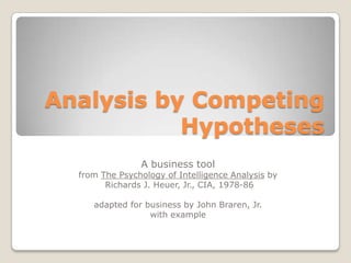
1. Analysis by Competing
Hypotheses
A business tool
from The Psychology of Intelligence Analysis by
Richards J. Heuer, Jr., CIA, 1978-86
adapted for business by John Braren, Jr.
with example
2. Why this presentation?
To put some extra time to good use while
between contracts, I decided to create
several presentations of some tools I believe
could be useful for business.
This is the first presentation.
I have made this as brief as possible in an
attempt to not kill interest, but I have no
doubt some points deserve more
development. Please feel free to contact me
at JBraren@nc.rr.com if you want to discuss
this further, or to offer comments to improve
the presentation and the clarity.
3. BI is probably wrong / FBDM
TMI- Too much information. Fact Based Decision
Making can mean more “volume” and less
“quality”.
Too many biases built in to collection
Programmed BI causes pre-filtering and
predetermined hierarchies and answers
Limits data with collection mechanisms
4. Current Process is troublesome
Select solution and find “proof”
This can yield the wrong answer for all the
right reasons
50:50 chance to get right answer - for all
the wrong reasons
5. Two bad examples
Wrong decision, for right reasons
Buy a copier that is cheap, saves $$ and ink, has small foot
print
But – can‟t print from remote, can‟t queue job for off-
hours, and only holds 100 sheets so need to monitor all
jobs
Right decisions, for wrong reasons
Build a bridge:
1- let‟s make out of steel, it‟s nice and shiny
2- I don‟t like driving over water, so let‟s put at
narrow point of river
3- Make lowest point of bridge at least 76‟ over water;
the mast on my sailboat is 72‟
6. So why does „satisficing‟ and
FBDM persist?
Habit and comfort
◦ More comfortable with failure than change
We are surrounded by the practice of
deciding and then developing CYA support
◦ Rather than stretching to find the most possibilities
and then expending effort to disprove most of them
More lucrative to sell BI tools and code than
a decision making skill
7. What is ACH?
Analysis by comparative hypotheses
Developed for the CIA in 1978 – 1986
Based on:
◦ - finding most possible answers
◦ - applying ALL pro/con data against ALL
hypotheses
◦ - disproving possibilities, not „proving‟
selections
8. The steps 1 – 4 of 8
1. Identify all the possible hypotheses to be
considered.
2. List all significant evidence and arguments for
and against. Combine to one matrix – all
evidence for all hypotheses.
3. Identify the evidence and arguments that were
most diagnostic.
a) All + or all – of no decision making value
4. Refine the matrix definitions as needed-
Hypothesis, Evidence, Original Question.
9. The steps 5 – 8 0f 8
5. Evaluate each hypothesis. Disprove hypotheses
and eliminate, rather than prove them.
6. Find the lynchpin items of evidence. Scrutinize
these.
e) The conflicting + and – decision points
7. Report the conclusions. Discuss the relative
likelihood of all the hypotheses, not just the most
likely one.
8. Identify milestones for future observation, to
monitor and re-evaluate analysis conclusions.
11. Which is best vest to buy?
V1 V2 V3 V4 V5 V6
Color F Orange F Orange F Green F Green Black Tan
Size Small All All All All All
Cost $1 $2 $3 $4 $ .10 $ .05
V5 and V6 might seem best buys, but colors don‟t seem right.
Need to add element of “Visibility”.
12. Which is best vest to buy? - 2
V1 V2 V3 V4 V5 V6
Color F Orng F Orng F Green F Green Black Tan
Size Small All All All All All
Cost $1 $2 $3 $4 $ .10 $ .05
Visibility 2 mile ½ mile ¼ mile 1 mile 1/100 1/100
mile mile
**With Visibility added, we see color isn‟t a decision factor.
**Small only size won‟t work for all our users, so eliminate V1. V5
and V6 are unacceptable distances, so eliminate these.
**V3 is less visible for more money than V2; eliminate V3
**And back to Visibility, what do we need? 1 mile for hunting season
or ½ mile for traffic visibility? This is our Lynchpin data.
13. A Real Example
The worst answer for all the best reasons
This real example works through a brief
version of the steps that went into making
a less valuable decision.
99+% consensus was the first decision was
best.
14. Where do we start a new business
system?
The three options were:
US based established company plant which
produces for largest (80% revenue) customer
Foreign established plant, no large customer
production
Newly acquired US plant, no large customer
production
15. The Evidence for hypotheses - #1
This was the evidence used to make the actual decision. It seems
to lead to an obvious conclusion (“new facility”) based on the
positive data. This was the path that was followed.
ACH forces the search for the lynchpin evidence and guards against
finding support for the obvious, which is too often wrong.
80% facilities Non-80% facilities New facilities, non-
80%
1. Can‟t afford to trouble
80% customer
_ _ __ ++ ++
2. Most of team from 80%
facility, want to avoid stress
n/a _ +
3. Need to learn new
system, so might as well do
n/a n/a ++
once
15
16. The Evidence for hypotheses - #2
With the help of hindsight, I have added the last three elements
of evidence to the matrix. If the search for evidence had been an
active exercise to consider all stake-holders and the complete
„state‟ of the implementation, these elements would have been
discovered and considered from the start.
80% facilities Non-80% facilities New facilities, non-80%
1. Can‟t afford to trouble 80%
customer
____ ++ ++
2. Most of team from 80%
facility, want to avoid stress
n/a _ +
3. Need to learn new system,
so might as well do once
n/a n/a ++
4. Employees feel pain, want
new system
+ + n/a
5. Employees need to keep
some of old, don‟t want new
n/a n/a _
system
6. Unique unfamiliar
measurement system
n/a n/a _
16
17. Evaluating Evidence through #2
1. The first hypothesis of starting with the 80% customer
facility has a huge negative and can be eliminated with
confidence. (Note that significance of evidence mat be
very subjective. If there is any doubt, the hypothesis
probably should be kept in play.)
2. If we look at evidence element 2 (team from 80%
facility), we can see that the evidence might be re-stated
as “Team from outside facility”, in which case it carries
the same negative (or positive) weight for both
remaining facility types.
3. And now elements 5 &6 add two negatives to the „new
facility‟ hypothesis which makes this our next best choice
to cut as an option.
4. But now we want to add a 7th piece of evidence.
17
18. The Evidence for hypothesis - #3
80% facilities Non-80% facilities New facilities, non-80%
1. Can‟t afford to trouble
80% customer
___ ++ ++
2. Most of team from 80%
facility, want to avoid stress
n/a _ _
3. Need to learn new system,
so might as well do once
n/a n/a ++
4. Employees feel pain, want
new system
+ + n/a
5. Employees need to keep
some of old, don‟t want new
n/a n/a __
system
6. Unique unfamiliar
measurement system
n/a n/a _
7. Rationalizations usually
add to scope, but:
Bringing facility into 80% n/a + +
methods will build “corporate
team” perception
18
19. Review each hypothesis
Review validity of each hypothesis; eliminate as
possible
Evaluating Evidence through #3
◦ Evidence elements 2 & 7 have equal values so they can
be eliminated as not useful.
◦ Because we are trying to disprove hypotheses, the two
negatives (elements 5 & 6) for “new facility” become the
only two valuable elements. These are the lynchpins.
19
20. The Conclusion
80% facilities Non-80% facilities New facilities, non-80%
1. Can‟t afford to trouble
80% customer
___ ++ ++
2. Most of team from 80%
facility, want to avoid stress
n/a _ _
3. Need to learn new system,
so might as well do once
n/a n/a ++
4. Employees feel pain, want
new system
+ + n/a
5. Employees need to keep
some of old, don‟t want new
n/a n/a __
system
6. Unique unfamiliar
measurement system
n/a n/a _
7. Rationalizations usually
add to scope, but:
Bringing facility into 80% n/a + +
methods will build corporate
team sense
20
21. Conclusion note - Item 4
80% facilities Non-80% facilities New facilities, non-80%
4. Employees feel + + n/a
pain, want new
system
Note that while this point may seem important, the fact is that it
was a non-starter from the beginning.
** With 2 “reasons for” and an “n/a” it had no dis-prove value.
** And even after eliminating the “80% facility”, it still had no
dis-prove value for the last two choices.
** This is a clear example where bias for a solution can be seen
as contrary to making a best choice decision.
21
22. ACH Steps Review
1. Identify all the possible hypotheses to be considered.
2. List all significant evidence and arguments for and against.
Combine to one matrix – all evidence for all hypotheses.
3. Identify the evidence and arguments that were most
diagnostic.
4. Refine the matrix- Hypothesis, Evidence, Original Question.
5. Evaluate each hypothesis. Disprove hypotheses and
eliminate, rather than prove them.
6. Find the lynchpin items of evidence. Scrutinize these.
7. Report the conclusions. Discuss the relative likelihood of all
the hypotheses, not just the most likely one.
8. Identify milestones for future observation, to monitor and
re-evaluate analysis conclusions.
23. Exercise
As a group, or individually, apply the ACH process to a
decision you might make, or best, to one decision that
worked and one that did not work.
The comparison of the historical decisions might drive
home the value of the ACH approach.
The exercise can be done quickly and still show its
value:
Identify question, refine, and follow through rest of
steps quickly
Best done on flip chart or white board, or an Excel
grid. Whatever works.
24. The Evidence for using ACH
Select and then find ACH Process
support
1. Find most possible
solutions or responses - ++
2. Disqualify options that do
- ++
not work
3. Keep options until they
are disproved; scientific - ++
4. Refine the question, the
evidence, and the solution - ++
throughout the process
5. Avoid bias - ++
24