AACE_Communicating expected estimate accuracy.pdf

1
0
4
R
-
1
9
C
O
M
M
U
N
I
C
A
T
I
N
GE
X
P
E
C
T
E
D
E
S
T
I
M
A
T
E
A
C
C
U
R
A
C
Y

Copyright © AACE® International AACE® International Recommended Practices
Single user license only. Copying and networking prohibited.
This document is copyrighted by AACE International and may not be reproduced without permission. Organizations may obtain permission
to reproduce a limited number of copies by entering into a license agreement. For information please contact editor@aacei.org
AACE® International Recommended Practice No. 104R-19
COMMUNICATING EXPECTED ESTIMATE ACCURACY
TCM Framework: 7.3 – Cost Estimating and Budgeting
Rev. February 22, 2021
Note: As AACE International Recommended Practices evolve over time, please refer to web.aacei.org for the latest
revisions.
Any terms found in AACE Recommended Practice 10S-90, Cost Engineering Terminology, supersede terms defined in
other AACE work products, including but not limited to, other recommended practices, the Total Cost Management
Framework, and Skills & Knowledge of Cost Engineering.
Contributors:
Disclaimer: The opinions expressed by the authors and contributors to this recommended practice are their own and do
not necessarily reflect those of their employers, unless otherwise stated.
Larry R. Dysert, CCP CEP DRMP FAACE Hon. Life
(Primary Contributor)
John K. Hollmann, PE CCP CEP DRMP FAACE Hon. Life
(Primary Contributor)
Dr. David T. Hulett, FAACE
Gordon R. Lawrence
Michael Lesnie
Michael L. Myers, PE CCP
Quinton van Eeden

AACE®
International Recommended Practice No. 104R-19
COMMUNICATING EXPECTED ESTIMATE ACCURACY
TCM Framework: 7.3 – Cost Estimating and Budgeting
February 22, 2021
TABLE OF CONTENTS
Table of Contents ..........................................................................................................................................................1
1. Introduction...............................................................................................................................................................2
2. Recommended Practice.............................................................................................................................................2
2.1. Definition of Uncertainty and Risk......................................................................................................................2
2.2. Definition of an Estimate....................................................................................................................................3
2.3. Definition of Estimate Accuracy..........................................................................................................................4
2.4. Presenting Estimate Accuracy ............................................................................................................................4
2.5 Estimate Accuracy and Estimate Classification..................................................................................................10
2.6. Estimate Accuracy and Risks.............................................................................................................................12
2.7. Estimate Accuracy and Quantitative Risk Analysis ...........................................................................................13
2.8. Estimate Accuracy as a Quality or Performance Measure................................................................................13
2.9. Estimate Accuracy as a Standard or Target ......................................................................................................14
3. Summary..................................................................................................................................................................15
4. References...............................................................................................................................................................16
5. Contributors.............................................................................................................................................................16
Appendix A...................................................................................................................................................................17
A.1. Probability Distributions...................................................................................................................................17

104R-19: Communicating Expected Estimate Accuracy 2 of 20
February 22, 2021
1. INTRODUCTION
This recommended practice (RP) of AACE International defines expected estimate accuracy; and describes how the
concept of estimate accuracy should be communicated to a stakeholder or decision maker that is interested in
understanding the potential variability or predictability that is associated with a particular estimate.
The results of the estimating process are often conveyed as a single value of cost or time. However, since estimates
are predictions of an uncertain future, it is recommended that all estimate results should be presented as a
probabilistic distribution of possible outcomes in consideration of risk. However, because probabilistic methods are
difficult to communicate, its concepts are reduced to an expression called expected estimate accuracy that is a
simplified means of communicating uncertainty as a single expression. Discussions of expected estimate accuracy
often describe estimate accuracy in terms of +/- percentages that bound the published single estimate value, but
too often fail to convey other significant information that is required by an estimate stakeholder to truly assess what
the +/- percentages indicate. Worse, rule-of-thumb percentages often fail to reflect the true risk and uncertainty at
all.
This RP applies to estimates of both cost and time (duration). Its subject matter deals with the integration of the
disciplines of decision and risk management, cost estimating and planning and scheduling within the AACE
International community. Where a discussion in the RP focuses on either cost or time specifically, it is noted as
appropriate.
This RP is intended to provide guidelines (i.e., not a standard) to be used in conveying the expected accuracy level
of an estimate to a stakeholder that are considered to be good practices that can be relied on and that would be
recommended for use where applicable. This RP will present an estimate as a probabilistic range of potential values
in consideration of risk, discuss the typical shapes of the probability distribution associated with the range of
potential values, discuss the concept of estimate contingency, and identify the elements required to convey
information about expected estimate accuracy to stakeholders. When referring to cost or duration estimating, this
RP focuses on cost or duration estimating for a project or dedicated effort to accomplish a scope of work or activities.
This RP does not discuss the calculation or determination of the variability of the indicated accuracy of an estimate
after completion of the associated project or effort (a comparison of an estimate with actual results). When the term
estimate accuracy is used in this RP, it is intended to convey expected estimate accuracy.
2. RECOMMENDED PRACTICE
2.1. Definition of Uncertainty and Risk
This RP addresses practices for communicating the probabilistic nature of estimates. As such, its subject matter
requires basic understanding of statistical and risk analysis concepts and terms. In particular, the following terms are
important to understand and will be discussed further in the RP:
• Error: where this term is used, it refers to its statistical meaning of error of prediction and does not mean a
mistake by the team or estimator unless so stated (although mistakes can be a contributing factor to error).
• Uncertainty: in respect to this RP, the term has two possible meanings. It can be used as a general synonym
for what the accuracy +/- range represents regardless of the cause of that range; or it may reflect the analyst
view that distinguishes between risk types wherein uncertainties are variability risks with 100 percent
probability of occurrence (i.e., not risk conditions and events).
• Risks: in respect to this RP, the term has two possible meanings. It can be used as a general synonym for
uncertainty and what the accuracy +/- range represents regardless of the cause of that range. Or, it may

February 22, 2021
reflect the analyst’s view that distinguishes between risk types wherein risks are identifiable conditions or
events with less than 100 probability of occurrence but contribute to error.
The fact that alternate definitions of uncertainty and risk are used and valid implies that those who communicate
about estimate accuracy must also communicate the meaning and context of these supporting terms.
2.2. Definition of an Estimate
AACE International defines an estimate as: A prediction or forecast of the resources (i.e., time, cost, materials, etc.)
required to achieve or obtain an agreed upon scope (i.e., for an investment, activity, project, etc.). [1] It applies to
both cost and time (duration).
AACE International defines a cost estimate as: The prediction of the probable costs of a project or effort, for a given
and documented scope, including a defined location and point of time in the future. [1]The results of a cost estimate
are expressed in a currency value.
In respect to cost, estimating is the predictive process used to quantify, cost, and price all of the resources required
by the scope of an investment option, activity, or project. [2] The output of the estimating process, the cost estimate,
is typically used to establish a project budget, but may also be used for other purposes, such as:
• Determining the economic feasibility of a project.
• Evaluating between project alternatives.
• Providing a basis for project and schedule control.
Activity duration estimating is defined as: Estimation of the number of work periods that will be needed to complete
the activity. [1]For duration (activity or project), the periods can be expressed in hours, days, months or any defined
time segment.
Every estimate is a prediction of the expected final cost or duration of a proposed project or effort (for a given scope
of work). By its nature, an estimate involves assumptions and uncertainties. Performing the work is also subject to
risk conditions and events that are often difficult to identify and quantify. Therefore, every estimate presented as a
single value of cost or duration will likely deviate from the final outcome (i.e., statistical error). In simple terms, this
means that every base estimate value will likely prove to be wrong. Optimally, the estimator will analyze the
uncertainty and risks and produce a probabilistic estimate that provides decision makers with the probabilities of
over-running or under-running any particular cost or duration value. Given this probabilistic nature of an estimate,
it should not be regarded as a single point cost or duration. Instead, an estimate actually reflects a range of potential
outcomes, with each value within this range associated with a probability of occurrence.
Typically, a single value (within the range of potential costs or durations) is communicated as the estimate value;
however, it is important for the estimator to convey the uncertainty associated with that single point value, to
describe the true probabilistic nature of the estimate, and the causes of the uncertainty to the estimate stakeholders.
In typical use, the point value represents either a base estimate value or an end use value. The base estimate is the
first value the estimator derives before considering and quantifying uncertainty and risks. The end use value includes
at least some consideration for uncertainty and risks and represents the estimate value applicable to a decision (e.g.,
authorization of funds, a bid price, approval of a schedule, etc.). In either case, a point value for an estimate (whether
the base or end use value) is in actuality just one point on a probability distribution curve that represents the range
of potential cost outcomes.
Most of the end uses of an estimate require a single point value within the range of probable values to be selected.
For example, at project sanction the funds to be authorized and acquired are represented by a single monetary
value. Likewise, for schedules a completion date representing a single duration value is communicated. When taking

February 22, 2021
into account the uncertainty associated with an estimate (including risk conditions and events), amounts known as
contingency and management reserve are added to base estimates to derive a single value suited for the end budget
or funding use. Note that depending on a specific organization’s polices, management reserve may be added to the
value of the base estimate or the value of the base estimate plus contingency. When determined effectively, the
end use value addresses uncertainty and risks considering stakeholder risk tolerance and confidence levels; and for
their purpose, represents the best single point value to support a project decision.
2.3. Definition of Estimate Accuracy
Accuracy is the degree to which an initial measurement or calculation varies to its final actual value. Accuracy is a
distinct and separate concept from precision. Precision is the degree to which a series of calculated values will show
similar results. Accuracy can be considered an expression or measure of predictability as well.
AACE International defines expected estimate accuracy as: An indication of the degree to which the value of a cost
or duration estimate may vary from the final actual outcome of the completed project or activity. [1]
As indicated above, an estimate should be regarded as a range of potential outcomes, with associated probabilities
of occurrence. Estimate accuracy is based on a probabilistic assessment of uncertainties and risks that forecasts how
far a project’s final cost may potentially vary from the single point value that is selected to represent the estimate,
whether a base estimate or end use value. The estimate range (the variability between the potential lowest
reasonable value for the estimate and the highest reasonable value) is driven by the uncertainties, and risks
associated with the project or activity being estimated.
2.4. Presenting Estimate Accuracy
Individual estimates should always have their accuracy ranges determined by a quantitative risk analysis study that
results in an estimate probability distribution when appropriate. The estimate probability distribution is typically
skewed. Research shows the skew is typically to the right (positive skewness with a longer tail to the right side of the
distribution) for large and complex projects. [3] In part, this is because the impact of risk is often unbounded on the
high side. For example, if a base estimate assumed 2 lost days of work per month due to weather based on local
historical data, the best would be 0 days, but the worst could be 10 or 20 or more.
High side skewness implies that there is potential for the high range of the estimate to exceed the median value of
the probability distribution by a higher absolute value than the difference between the low range of the estimate
and the median value of the distribution. When a probability distribution is positively skewed, the median is a higher
value than the mode, and the mean is typically higher than the median (see the appendix information on probability
distributions). Some complex projects may have bi-modal, long and/or fat tails or other unusual distributions
depending on the nature of the risks.
Some skewness may be due to bias in the base estimate. For example, small projects and others with less pressure
on cost and more on safety or other objectives are often estimated with a conservative bias to minimize the
bureaucratic entanglements that cost overruns may provoke. These may display skewness to the left; a tendency to
underrun. On the other hand, as projects become larger and the focus on minimizing costs becomes greater, the
base estimate may have an aggressive bias (optimism bias). Bias should be minimized, but one must assume that
every base estimate has some bias, and risk analysis must attempt to identify and quantify it (the topics of estimate
validation and benchmarking are covered in other RPs).
Figure 1 shows a positively skewed distribution for a sample cost estimate risk analysis that has a base estimate (the
value before adding contingency) of $88.5. As illustrated in Figure 1, typically the value of the base estimate before

February 22, 2021
contingency is less than the mode, median and mean values of the distribution.1
Also, note that the tails of the
distribution in this example range from $80 to $115, and there would be a temptation to describe the estimate range
as between $80 and $115 with 100% certainty. Note: Many of the figures included in this RP were created using
Palisade @Risk for Excel, Version 6.3.1 Professional Edition.
Figure 1 – Sample Estimate Probability Distribution with a Base Estimate before Contingency of $88.52
It is not best practice, however, to express the potential range of the estimate with 100% certainty because it implies
specific absolute limits to potential underrun or overrun of the estimate value. Although the calculated probability
distribution from the estimate risk analysis may identify absolute lower and upper bounds, it is unrealistic to specify
absolute limit to the tails of the estimate probability distribution in actual practice (See Figure 2). This does not imply
that the lower and upper bounds of the estimate are indefinite (i.e., that the costs are unbounded); but that the
specific lower and upper values of the estimate range are indeterminate for the purposes of risk or uncertainty
assessment.
1
The point value (before consideration of risk and uncertainty for the estimate) will typically lie to the left of the mode of the resulting cost
probability distribution from a risk analysis. Although an estimator may (in theory) select a most-likely or mode value for individual items in an
estimate, that value is usually selected without consideration of the estimate-wide systemic and project-specific risks and uncertainties. Thus, a
level of contingency is required to achieve the most-likely (mode) value of the estimate total (in consideration of project risks); and since the
cost distribution is typically skewed, additional contingency is required to achieve the p50 (median) or the mean value of the cost distribution
resulting from risk analysis (to the right of the mode). Also, note that the most-likely (mode) values for individual estimate items comprising the
estimate are also typically based on skewed distributions for each of those individual items. One cannot add the mode values of the individual
items to obtain the mode value of the overall estimate (only the means of individual cost distributions are additive for anything other than
normal or other symmetrical distributions).
2
Note that the probability distribution graphics in this RP are shown as relative frequency probability distributions, not cumulative probability
distributions. The skewness of the distribution is more easily recognized and displayed in a relative frequency distribution, which is important to
this discussion of estimate accuracy. In a formal risk analysis report, it may be more prevalent to display risk results as a cumulative probability
distribution. The advantage of a cumulative probability distribution in reporting of risk analysis results is that many will find it easier to
associate a cost value with a given level of underrun (P value), as the y-axis of a cumulative probability distribution ranges from 0% probability
of underrun to 100% probability of underrun. The y-axis of a relative frequency distribution identifies the central tendencies and skewness of
the distribution, but the values of the y-axis are not meaningful.

February 22, 2021
Figure 2 – The Tails of the Probability Distribution
In fact, research shows that even the best analyses are poor predictors of the extreme tails; and final high-end
outcomes at the 100% confidence interval (worst case) are often many multiples of the base estimate value (i.e., the
high tail is for practical purposes unbounded and asymptotic). [3] For those reasons, estimate ranges should never
be expressed with 100% confidence interval. The estimate range should typically be presented with no better than
a 90% confidence interval (the range between the P5 and P95 confidence level values of the estimate probability
distribution) and more practically at an 80% confidence interval (between the P10 and P90 confidence level values
of the distribution). The evaluation of uncertainty and risk identification (including assessment of the probabilities
of risks occurring and the range of potential impact to cost or duration should they occur) is itself a stochastic process
subject to uncertainty. Indicating extremely high confidence levels (higher than 90%) would imply a level of precision
to risk analysis and the resulting cost distribution that is unrealistic.
For example, as shown in Figure 3, it can be stated that there is a 90% confidence that the final outcome will be
between $85 and $103, considering appropriate rounding.

February 22, 2021
Figure 3 – Estimate Range at a 90% Confidence Interval
As shown in the previous figures, the point base estimate before including contingency typically has a relatively small
probability of underrun and a large probability of overrun. This is due to the fact that base estimates by design should
exclude risks (though they have inherent uncertainties) that are addressed by the quantitative risk analysis study
used to model the estimate probability distribution associated with the estimate. [4] Therefore an amount of money
is typically added to the point base estimate value to improve the probability of not overrunning the final end use
value (or improve the probability of underrun).
For example, in Figure 4, a contingency of $4.5 (approximately 5%) is required to achieve a 50% probability of
underrun, which increases the final end use value to $93. Note that this RP is intended to describe the concepts but
not to recommend specific confidence levels for funding contingency or management reserves of particular projects;
that depends on the stakeholder risk attitude and tolerance.

February 22, 2021
Figure 4 – Adding Contingency to Achieve a P50 Value of Underrun versus Overrun
Note that adding contingency to the base point estimate does not affect estimate accuracy in absolute terms as it
has not affected the estimate probability distribution (i.e., high and low values are the same). Adding contingency
simply increases the probability of underrunning the final end use estimate value and decreases the probability of
overrunning the final estimate value. In Figure 4, the estimate range with a 90% confidence interval remains between
$85 and $103 regardless of the contingency value.
Contingency in this context is the funds or time required to be added to the original point base estimate to achieve
a given probability of not overrunning the estimate within the defined project scope. Typically, the value of
contingency will be established as the amount of funds or duration to reach the mean value of the probability
distribution; or more commonly to reach the P50 (median) value of the probability distribution (which is close to the
mean for most distributions). Using the mean value for contingency determination has an advantage across a
portfolio of projects because the means of probability distributions can be additive, whereas medians of probability
distributions are not.3
When contingency is determined at the mean or P50 values of the probability distribution, it
should be expected that it will be expended during project execution (i.e., it is not considered a slush fund).
If a greater value is chosen as the end use value for the estimate, (a value greater than the mean or P50 value) to
provide an acceptable level of risk to the stakeholder, then the difference between that greater amount and
contingency is often designated as management reserve. In bidding or pricing, it may represent a margin. Typically,
management (whether project management or corporate management) establishes the acceptable level of risk, and
hence the final end use value for the estimate. The estimator’s role is limited to developing the base estimate and
supporting the quantitative risk analysis to communicate meaningful information to the decision maker.
Figure 5 illustrates expressing estimate accuracy as a percentage range for a given point value. In this example, when
estimate accuracy is expressed as a percentage range at a 90% confidence interval, the estimate accuracy range
3
For a positively skewed distribution, the mean will be greater than the median as it is more highly weighted by the extreme high values at the
right tail of the distribution. For a typical skewed cost risk analysis, the mean tends to lie around the P55 to p60 point (55% to 60% probability
of underrun) of the cost distribution. [3] When the cost distribution is highly skewed, it may be preferred to select the mean value of the cost
distribution for contingency determination rather than the median value.

February 22, 2021
around the P50 estimate value of $93 is approximately -8% / +10%. Note that one should avoid too much precision;
the methods are stochastic and arguably one should limit reported values to two or three significant figures.
Figure 5 – Expressing Estimate Accuracy in Percentage Terms around the P50 Estimate Value
When expressing estimate accuracy in terms of percentages, both the confidence interval and the reference
estimate value upon which the percentage range is based must be specified. As an example of why one must state
these conditions, consider Figure 6. In this example, the end use value of the estimate has been increased to the P70
confidence level of $96.0 (which may include both contingency and management reserve funds).

February 22, 2021
Figure 6 – Expressing Estimate Accuracy in Percentage Terms around the P70 Estimate Value
In Figure 6, when estimate accuracy is expressed as a percentage range, the 90% confidence interval around the P70
confidence level of $96.0 is approximately -11% / +7% compared to the -8% / + 10% in Figure 5 around the P50
reference value. Figures 5 and 6 show two different percentage ranges for the same estimate distribution; if one did
not explain what the reference point (confidence level) was and the confidence interval, the estimate accuracy range
in percentage terms may be misleading or misinterpreted. It is recommended to always communicate the estimate
accuracy range in terms of absolute values for a declared confidence interval.
2.5 Estimate Accuracy and Estimate Classification
Expected estimate accuracy tends to improve (i.e., the range of probable values narrows) as the level of project
scope definition improves. In terms of the AACE International estimate classifications, increasing levels of project
definition are associated with moving from Class 5 estimates (lowest level of scope definition) to Class 1 estimates
(highest level of scope definition). This concept is illustrated in Figure 7.

February 22, 2021
Figure 7 – Estimate Accuracy Improves as the Level of Project Definition Improves
Figure 7 is intended to illustrate only the general relationship trend between estimate accuracy and the level of
project definition. As described in the AACE International recommended practices on estimate classification, there
is no absolute, pre-determined standard range for any estimate or class of estimate. As an example, for the process
industries, typical estimate ranges described in RP 18R-97: Cost Estimate Classification – As Applied in Engineering,
Procurement, and Construction for the Process Industries [5] are illustrated as a range of ranges (there are RPs that
cover other industries that may have different values):
• Class 5 Estimate
• High range typically ranges from +30% to +100%
• Low range typically ranges from -20% to -50%

February 22, 2021
Note that these +/- percentage measures associated with an estimate class are intended as rough indicators of the
accuracy trend provided the company and project are well managed and no major risks occur. These are merely a
useful simplification given the reality that every individual estimate will be associated with a unique probability
distribution explaining its unique level of uncertainty and risk that must be determined through a quantitative risk
analysis for each particular estimate. Note that the estimate classification RPs provide +/- percentages around the
reference estimate including contingency to obtain a 50% probability of underrun/overrun and an 80% confidence
interval. This does not preclude a specific actual project result from falling inside or well outside of the indicated
accuracy range of ranges in the appropriate industry classification RPs. In fact, research indicates that for weak
project systems and complex or otherwise risky projects, the high ranges may be two to three times the high end of
the classification RP values (this can be mitigated somewhat by allowing for very high contingency). [3]
2.6. Estimate Accuracy and Risks
Although level of project definition (generally correlated with percent of engineering complete) is an important
determinant or risk driver of estimate accuracy, there are many other uncertainty and risk drivers that also affect
accuracy. In respect to risk quantification methods, AACE International defines three main types of risks: systemic,
project-specific, and escalation (including currency where applicable). All must be considered. Keeping in mind that
expected estimate accuracy is an expression of an estimate’s predicted closeness to the final actual value; anything
included in that final actual, be it the result of general uncertainty, risk conditions and events, price escalation,
currency or anything else within the project scope, is something that estimate accuracy measures must
communicate in some manner. With that in mind, it should be clear why standard accuracy range values are not
applicable to individual estimates.
The level of project definition reflected in the estimate is a key risk driver and hence is at the heart of estimate
classification. The level of scope definition is called a systemic risk because it is usually a key objective of project
phase-gate systems. Systemic risks are attributes of the project system that result in uncertainty. As attributes, they
are simply elements that can be rated or measured, i.e., their probability of occurrence is 100% (some might call
them issues). The weaker and more unreliable the project system, including definition, the more risk there is and
the less accuracy there will be. Some of these systemic risks or factors include the strength of team development
(i.e., are roles filled, is competency high, etc.), the maturity of the project process, the maturity and capabilities of
the project control process and systems, and so forth. Also, the higher the level of technology and complexity in the
project scope, and complexity of the execution strategy, the greater the uncertainty. Probability of occurrence of
systemic risks is 100%. The range of potential impact on an estimate will vary based on the factors such as those
discussed above and requires careful evaluation in the risk analysis process.
A subset of systemic risks, as an element of project process maturity and capability, is what can be called estimating
process uncertainty. Included in this category are:
• The quality of the quantity takeoffs.
• The quality of reference estimating data (for cost, material pricing, labor hours, labor wage rates, etc.).
• The quality of the assumptions used in preparing the estimate.
• The experience and skill level of the estimator.
• The degree of integration of estimating with scheduling and other project functions.
• The reliability of the specific estimating techniques and tools employed.
• The level of effort budgeted to prepare the estimate.
Estimating process uncertainty will be discussed later in respect to using estimate accuracy as targets.
Other risk drivers include project-specific risks. These are conditions or risk events such as the possibility of
discovering unanticipated rock in the soil, the occurrence of an unusual weather event, or a piece of critical
equipment falling off a truck and being damaged. Typically, the probability of occurrence is less than 100 percent. A

February 22, 2021
project system attribute that changes during the course of a project could be considered a risk event as well (e.g., a
strong project team is in place at kick-off, but turnover in key roles occurs during execution). Risk management
processes themselves, including the ability of the project team to effectively manage identified risks and
opportunities, must also be considered in evaluation of project uncertainty.
The last major type of risk is escalation and currency exchange. These include economic driven changes in prevailing
price levels and changes in the relative value of currencies used. The longer the project duration and more volatile
the economy, the greater these risks are. Often, the ownership of these external risks is assumed by company
finance, i.e., the project is indemnified such that their impact to the final cost is corrected for, and therefore may
not play into the accuracy question. It is important to clearly state if these risks are or are not included when
discussing accuracy ranges.
In short, given all these sources of uncertainty and risks, it is simply not possible to define a range of estimate
accuracy based solely on the level of project definition or class of estimate. It is possible to have a Class 5 estimate
with a very narrow estimate accuracy range, particularly for repeat projects with good historical costs upon which
to base the estimate. Conversely, it is possible to have a Class 3 or Class 2 estimate with a very wide accuracy range,
particularly for first-of-a-kind projects, those employing new technologies, or those with untested execution
strategies or high complexity.
When discussing estimate accuracy, it is also important to realize that for early conceptual estimates, variations or
lack of clarity in the design basis will have the greatest impact on costs. Estimating tools and methods, while
important, are not usually the main problem during the early stages of a project when estimate accuracy is poorest.
In the early phases of a project, effort should be directed towards establishing a better design basis, and historical
data aligned with that, than concentrating on utilizing more detailed estimating methods in order to improve
estimate accuracy.
2.7. Estimate Accuracy and Quantitative Risk Analysis
Quantitative risk analysis is a process that applies a scientific approach to understanding the uncertainties and risks
associated with the cost and schedule of a project and generating the estimate probability distributions for cost and
duration. When prepared effectively, it not only supports the determination of the amount of contingency and
management reserves to be added to a base estimate to provide an acceptable confidence level of underrun, but
clearly identifies the risks driving the probability distribution so they can be managed. The quality management
practices of estimate validation and benchmarking should be allied with risk analysis because they objectively
identify and quantify the bias risk in the estimate. AACE International has several recommended practices for
integrated project cost and schedule risk quantification as well as validation and benchmarking; they are not covered
in this RP. The key point is that risk quantification results in the probabilistic distribution and hence the measure of
estimate accuracy.
2.8. Estimate Accuracy as a Quality or Performance Measure
A project that produces all of the technical and project deliverables required for a particular estimate class, and that
has good quality cost reference information, project history to rely on, and mature estimating and risk management
processes and methods will tend to have narrower estimate accuracy ranges than projects without them. Similarly,
an organization that consistently supports and delivers strong capabilities to its project teams will have narrower
accuracy ranges for its portfolio. As such, many companies use estimate accuracy as a quality measure or key
performance indicator (KPI) for its projects and project system (i.e., the portfolio of projects). For example, a goal to
achieve +/- 10% accuracy on individual projects is often observed. For a portfolio, the finance function is often a
particularly strong advocate of such a measure given that stockholders see capital spending predictability as a KPI.

February 22, 2021
However, caution must be used in applying estimate accuracy as a predictability metric. The problem is that used
alone, the easiest way to achieve tight accuracy and predictability is to over-estimate the project (often
subconsciously) and execute the project while spending the inflated budget. This padding also detracts from project
control discipline. Over estimation is known to be a common result of using estimate accuracy as a single KPI. The
recommended practice is to also measure cost or capital effectiveness or competitiveness which is a measure of
achieving lower absolute cost for the same scope over time, or in comparison to peer companies. Using predictability
and competitiveness KPIs together in consideration of management’s risk tolerance tempers potential incentive to
over-estimate.
A worse practice is using estimate accuracy as an element of employee (usually the estimator, but sometimes the
entire project team) performance rating. As discussed, estimate accuracy is driven by many risks for which the
estimator and project team have little control and feeble methods to predict their occurrence or impact. Using
accuracy as a personal performance measure is almost guaranteed to result in over-estimation.
2.9. Estimate Accuracy as a Standard or Target
Related to the topic of KPIs, many if not most companies have established their own standard estimate accuracy
ranges. These are usually documented as part of the company’s stage or phase-gate project scope development and
planning process, sometimes called a Front-End Loading (FEL) or Front-End Planning (FEP) process. AACE
International estimate classes are intentionally designed to support phase-gate systems. Typical ranges one may find
specified by companies are +100/-50% for Class 5, +30/-15% for Class 4 and +15/-10% or tighter for Class 3. Prior to
1997, AACE literature also quoted ranges such as this, but they were replaced by range-of-ranges with development
of the classification RPs because it became clear that fixed ranges were being misinterpreted and causing distortions
in risk analysis and ultimately contributing to worse project outcomes (re: the KPI discussion). Also, as projects have
grown in size and complexity, these legacy ranges are often understated by a factor of 2 to 3 (e.g., +250/-50% at
Class 5 is not uncommon for a new technology or very complex project even with a generous contingency).
As quantitative risk analysis practices evolved, research showed that seemingly sophisticated project cost risk
analyses were generating probability distributions that replicated the misinterpreted standards regardless of the
risks that were identified. [6] Just as estimators are incentivized to over-estimate costs and duration when accuracy
KPIs are used alone, risk analysts are incentivized to meet management expectations communicated via fixed
accuracy standards. It can be much more convenient to bias a risk analysis (e.g., simply ignore key risk drivers such
as a weak project system) then to treat the risk (e.g., to improve the project system). Given methodological
complexity, bias can readily enter the risk analysis, usually subconsciously. As such, it is recommended that such
accuracy range standards either not be quoted, or explicitly defined as indicators of relative phase-gate accuracy
progression (i.e., from Class 4 to Class 3 one should expect accuracy range span to tighten by a factor of about 2). If
quoted they should at least be based on empirical research of one’s actual experience. They should not be used as
KPIs, personal performance rating metrics, or hard targets.
For example, if a quantitative risk analysis of a project at a Class 3 level of scope definition is +32/-18% around the
base estimate with contingency at an 80% confidence interval, then that is what it is for the identified risk. It does
not necessarily reflect a poor project system, a bad estimate, or an unskilled estimator. If the company has a target
of +15/-10% at Class 3 and management will not accept a wider range for an individual estimate, the only way to
achieve improving the estimate accuracy range is to recycle the project through improved planning and scope
definition deliverables to support the estimate, and to treat and manage the risks (e.g., mitigate, transfer, etc.)
accordingly. If the indicated cost at the high end of the probability distribution (to achieve a high probability of
underrun) is too much to meet project economics, then the project should consider changing scope, not changing
the estimate.
That is not to say the legacy standard ranges have no meaning. They were originally intended to reflect the
estimating process uncertainty discussed previously (a subset of systemic risks). In other words, if the project system

February 22, 2021
is mature and strong, no significant design changes are made, no significant risk events occur, there is no new
technology and low complexity, execution performance is good, and the economy and markets are stable, these
legacy ranges can reasonably be expected. They represent the range of uncertainty resulting from the estimating
process alone (i.e., the takeoff, pricing quality, assumptions, methods used, etc.). Unfortunately, management and
decision makers often do not interpret them in such a narrow way, so it is better to avoid the risk of incentivizing
biased estimating and risk analysis by not quoting such pre-determined accuracy ranges.
3. SUMMARY
All cost estimates are predications that involve uncertainties and risks (and this exists for virtually all individual
elements of the estimate as well). This uncertainty means that an estimate result must be presented probabilistically.
All cost and duration estimates should reflect a range of potential outcomes that need to be effectively
communicated to the estimate stakeholders along with the causes of the range.
Formal quantitative risk analysis should always be used to determine the estimate probability distribution associated
with a specific estimate. This supports determination of the contingency and management reserve required to select
the single value for the project budget and completion date based on the level of confidence or risk acceptable to
management.
When describing estimate accuracy range to stakeholders, identify the confidence interval (typically 80% or 90%)
associated with the estimate range between the indicated lower and upper absolute cost or duration values. If the
estimate range is presented as a +/- percentage, then the reference point must be also be defined that the
percentage variations represent (e.g., the base estimate or end use value). If a single end use value is stated, the
probability of underrun (confidence level) associated with that value must also be stated.
The estimate accuracy range-of-ranges percentages described in AACE International estimate classification
recommended practices are intended only as an illustration of the general, relative relationship between estimate
accuracy and the level of project definition (and thereby class of estimate); and should not be relied upon for an
individual estimate. It is not possible to define a precise range of estimate accuracy based solely on the level of
project definition or class of estimate. Any specific estimate may not exhibit the patterns described in an estimate
classification recommended practice and should always have its accuracy determined through a quantitative risk
analysis process.
Every base estimate should reliably predict the costs to deliver the project or effort, given the scope and assumptions
reflected in the estimate and stated in the basis of estimate, but not considering risk. Every final estimate should
reflect a probabilistic outcome considering all identified risks including bias (bias is not desirable, but common and
should be addressed explicitly). Estimate uncertainty is reflected in the estimate probability distribution and
resulting estimate accuracy range derived from a risk analysis study for the specific estimate. Care should be taken
when using accuracy as a quality or performance measure, or target accuracy ranges by class, as that practice often
results in bias and loss of integrity in the estimating, risk analysis, and even the project control process. Quoting
standard or pre-determined accuracy ranges for individual estimates or estimate classes is discouraged.
The estimate should provide sufficient accuracy to support the decision and level of risk tolerance at hand. To
improve estimate accuracy, the project scope as reflected in the technical and project deliverables supporting the
estimate, and/or the capability of the project system and organization must be improved, and/or other risks treated,
to reduce risks and uncertainty. Accuracy cannot be significantly improved by the estimator doing a better estimate.
Properly quantified, interpreted and communicated, accuracy is a key measure supporting the predictability aspect
of achieving more profitable or capital effective outcomes.

February 22, 2021
4. REFERENCES
[1] AACE International, Recommended Practice No. 10S-90, Cost Engineering Terminology, Morgantown, WV:
AACE International, Latest revision.
[2] L. R. Dysert, "(EST.01) Is "Estimate Accuracy" an Oxymoron?," in AACE International Transactions,
Morgantown, WV, 2006.
[3] J. K. Hollmann, Project Risk Quantification, Sugarland, TX: Probabilistic Publishing, 2016.
[4] AACE International, Recommended Practice No. 40R-08, Contingency Estimating – General Principles,
Morgantown, WV: AACE International, Latest revision.
[5] AACE International, Recommended Practice No. 18R-97, Cost Estimate Classification System – As Applied in
Engineering, Procurement, and Construction for the Process Industries, Morgantown, WV: AACE International,
Latest revision.
[6] S. E. Burroughs and G. Juntima, "(EST.03) Exploring Techniques for Contingency Setting," in AACE International
Transactions, Morgantown, WV, 2004.
[7] AACE International, Recommended Practice No. 66R-11, Selecting Probability Distribution Functions for Use in
Cost and Schedule Risk Simulation Models, Morgantown, WV: AACE International, Latest revision.
[8] D. Vose, Risk Analysis: A Quantitative Guide, Third ed., West Sussex, England: John Wiley & Sons Ltd., 2008.
[9] H. L. Stephenson, Ed., Total Cost Management Framework: An Integrated Approach to Portfolio, Program and
Project Management, 2nd ed., Morgantown, WV: AACE International, Latest revision.
5. CONTRIBUTORS
Disclaimer: The opinions expressed by the authors and contributors to this recommended practice are their own and
do not necessarily reflect those of their employers, unless otherwise stated.
Larry R. Dysert, CCP CEP DRMP FAACE Hon. Life (Primary Contributor)
John K. Hollmann, PE CCP CEP DRMP FAACE Hon. Life (Primary Contributor)
Dr. David T. Hulett, FAACE
Gordon R. Lawrence
Michael Lesnie
Michael L. Myers, PE CCP
Quinton van Eeden

February 22, 2021
APPENDIX A.
A.1. Probability Distributions
This appendix will provide a short primer on probability distributions. Please reference a probability and statistics
text for a more thorough understanding of the concepts. Also, AACE RP 66R-11 [7] describes probability distribution
functions often used for cost and schedule risk simulation modeling.
David Vose states that “probability is a numerical measurement of the likelihood of an outcome of some stochastic
process”, and defines a probability distribution as describing the “range of values the variable may take, together
with the probability (likelihood) that the variable will take a specific value.” [8] When displayed graphically, a
probability distribution shows the range of possible values for a variable along the x-axis, and the probability of
occurrence (or relative probability of occurrence) along the y-axis.
Probability distributions may be discrete, which describes a distribution where only specific values within the range
may be possible (e.g. the roll of a die can only be integer values from 1 to 6); or continuous where any value within
the range may be possible (e.g. the result of an estimate risk analysis where any value between the range of $80 and
$115 may be possible, as illustrated in Figure 1).
For continuous probability distribution, the shape of the probability density curve may take many different shapes;
some are shown in the following examples.
Figure 8 shows a uniform distribution, where the variable may take any value within the range of 80 and 120. Every
value between (and including) 80 and 120 have an equal probability of occurrence. Note that for a continuous
probability distribution, the y-axis values are essentially meaningless. They are completely dependent on the number
of bins or x-axis sub-ranges used to create the graphic. In this case, the x-axis was developed with 40 sub-ranges
with each sub-range (e.g. between 80 and 81, or between 90 and 91) having a 2.5% probability of occurrence. Any
specific x-axis value, such as 87.3645, has an infinitesimally small value of occurrence; which is why the y-axis is often
referred to as showing relative probability.
Figure 8 – Example Uniform Probability Distribution

February 22, 2021
Figure 9 illustrates a normal probability distribution, with a range from 80 to 120; and a mean, median, and mode
value of 100 (it is symmetrical). A normal distribution is often referred to as a bell curve. A normal probability
distribution exhibits the concept of central tendency, where the probability of occurrence for values within the range
tend to be higher for some value near the center of the distribution. The mean is the probability-weighted average
of the distribution (or expected value). The median (also known as the P50 value) is the value at which there is an
equal 50/50 chance of an actual occurrence for the variable being below or higher than the median value. The mode
is the (typically single) value that has the highest probability of occurrence. In a normal (or uniform) distribution, the
mean, median and mode values are equal.
When a Pxx value is referred to, it references the value of the distribution at which xx% of the values of the
distribution lie at or below the Pxx value. Therefore, a P10 value of a probability distribution is that value where 10%
of the possible values lie at or below the P10 value (i.e. 10% of the area under the probability distribution curve lie
to the left of the P10 value). Similarly, 90% of the possible values of the distribution lie to the left of the P90 value
of the distribution.
Figure 9 – Example Normal Probability Distribution
Figures 10 and 11 illustrate skewed distributions. Skewness is a measure of how lopsided a probability distribution
may be. Positive skewness indicates a long right tail to the distribution; and negative skewness indicates a long left
tail to the distribution.

February 22, 2021
Figure 10 – Example Positive (Right) Skewed Distribution
Figure 11 – Example Negative (Left) Skewed Distribution
Note that in Figures 10 and 11, the probability distributions are shown as histograms rather than continuous curves.
The probability distributions that result from Monte Carlo risk analysis simulations are histograms that indicate the
number of bins (or sub-ranges of x-axis values) used to create the graphic, and from which a curve can be generated.

February 22, 2021
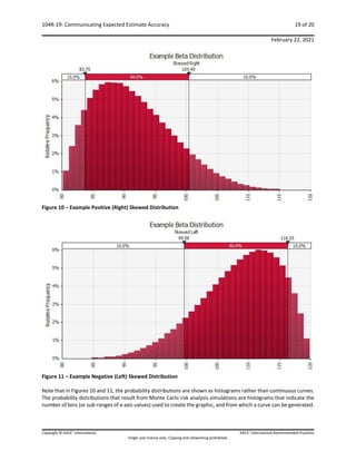
In skewed distributions, the mean, median and mode will usually be different values. When a probability distribution
is positively skewed, the median is a higher value than the mode, and the mean is typically higher than the median
(refer to Figure 1). For the results of a risk analysis to determine estimate accuracy, the mean and the median are
the most important measures of central tendency. The indicated mode from a risk analysis can only indicate the area
in which most of the values lie, since the probability of any one specific value occurring is so small.
Many organizations will budget at the P50 value (median) of a resulting estimate risk analysis but should be aware
that the P50 value is less than the expected value (mean) of the risk analysis results. The more skewness, the greater
the difference (the mean can be said to be more risk weighted). So, funding at P50 may still result in overrunning
the budget even when risk is adequately managed and controlled. The mean has an additional advantage of being
additive for a portfolio.
Many studies support the overall positive skewness to estimate accuracy for large projects. However, small project
systems often have an overall negative skewness implying that small maintenance projects (or others whose cost do
not have much individual impact on capital budgets) are often over-estimated within many operating owner
organizations. Care should be taken to understand this dichotomy. Further, some project risk profiles may result in
bimodal or other non-linear risk outcomes; a condition that simplistic accuracy ranges do not communicate well. [3]

AACE_Communicating expected estimate accuracy.pdf

More Related Content

Similar to AACE_Communicating expected estimate accuracy.pdf

Recently uploaded

AACE_Communicating expected estimate accuracy.pdf