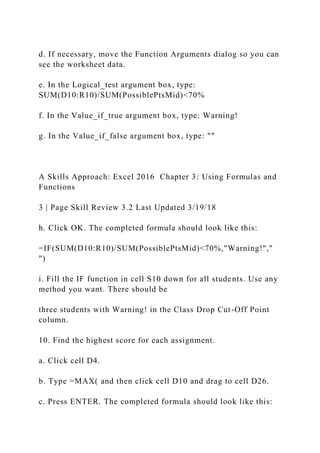
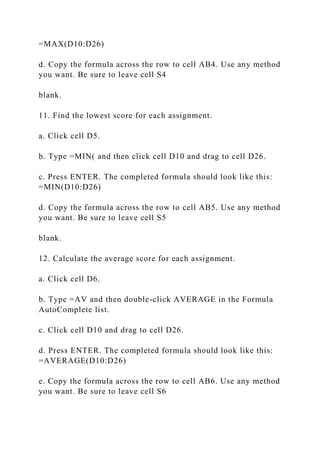
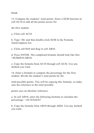
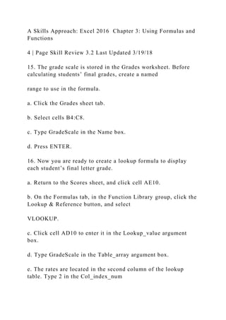
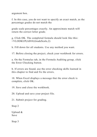
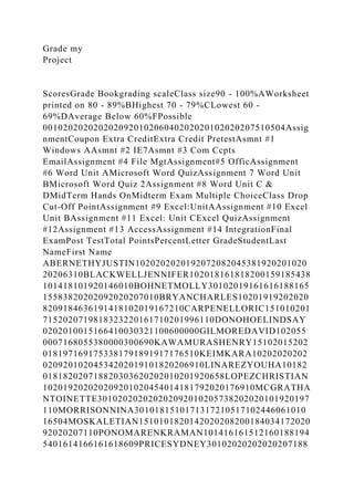
A Skills Approach: Excel 2016 Chapter 3: Using Formulas and
Functions
1 | Page Skill Review 3.2 Last Updated 3/19/18
Skill Review 3.2
In this project you will edit a worksheet to compute student
grades and grade statistics. Be sure to save your
work often!
Skills needed to complete this project:
• Using Date and Time Functions
• Using CONCAT to Combine Text
• Formatting Text Using Functions
• Creating Formulas Using Counting Functions
• Using Formula AutoComplete to Enter Functions
• Displaying and Printing Formulas
• Naming Ranges of Cells
• Using the Logical Function IF
• Using the Function Arguments Dialog to Enter Functions
• Working with Named Ranges
• Finding Minimum and Maximum Values
• Calculating Averages
• Finding Data Using the VLOOKUP Function
• Checking Formulas for Errors
1. Open the start file EX2016-SkillReview-3-2. The file will be
renamed automatically to include your
name. Change the project file name if directed to do so by your
instructor, and save it. Click the Enable
Editing button in the Message Bar at the top of the workbook so
you can modify it.
2. Take a look at the two sheets. The first sheet contains the
students' names and their scores. The second
sheet will be used to look up the letter grade for each student.
3. On the Scores worksheet, enter a function in cell B3 to
display the current date and time.
a. If necessary, click the Scores worksheet tab. Click cell B3.
b. On the Formulas tab, in the Function Library group, click the
Date &Time button.
c. Click NOW.
d. Click OK.
4. The first column should display the full student name. Use
CONCAT to combine the values from the
First Name and Last Name columns.
a. Click cell A10.
b. On the Formulas tab, in the Function Library group, click the
Text button, and select CONCAT.
IMPORTANT: If you do not see CONCAT in the list, use
CONCATENATE function instead.
c. Click cell C10 to enter the cell reference in the Text1
argument box.
d. Press TAB to move to the Text2 argument box.
e. Type " " to place a space between the first and last names.
f. Press TAB to move to the Text3 argument box.
Step 1
Download
start file
A Skills Approach: Excel 2016 Chapter 3: Using Formulas and
Functions
2 | Page Skill Review 3.2 Last Updated 3/19/18
g. Click cell B10 to enter the text reference in the Text3
argument box.
h. Click OK. The completed formula should look like this:
=CONCAT(C10," ",B10)
5. Add the PROPER function to the formula so student names
do not appear in all uppercase.
a. Double-click cell A10 to edit the formula.
b. Create a nested formula by typing PROPER( between the =
symbol and CONCAT.
c. Type another ) at the end of the formula.
d. Press ENTER. The completed formula should look like this:
=PROPER(CONCAT(C10," ",B10))
e. Copy the formula from cell A10 to A11:A26 to fill the list of
student names. Use any method you
want.
6. Count the number of students to calculate the class size.
a. Click cell B2.
b. Type =COU
c. Double-click COUNTA in the Formula AutoComplete list.
d. Click cell A10 and drag to cell A26.
e. Press ENTER. The completed formula should look like this:
=COUNTA(A10:A26)
7. Display your formulas to check for accuracy.
a. On the Formulas tab, in the Formula Auditing group, click
the Show Formulas button.
b. When you are ready to continue, hide the formulas and
display formula values by clicking the Show
Formulas button again.
8. Define a named range for the total possible points up to the
class drop cut-off point.
a. Select cells D7:R7.
b. In the Name box, type: PossiblePtsMid
c. Press ENTER.
9. Find out which students have a grade below C at the cut-off
point for dropping the class. Enter an IF
function in cell S10 to check if the student’s total points
divided by the total possible points through the
midterm is less than 70% (the lowest percentage for a C grade).
Use SUM functions within the IF
function. Be sure to use the range name you just defined for
possible points. If the student is below a C
grade, display Warning! in the cell; otherwise leave the cell
blank.
a. Click cell S10.
b. On the Formulas tab, in the Function Library group, click
Logical.
c. Click IF.
d. If necessary, move the Function Arguments dialog so you can
see the worksheet data.
e. In the Logical_test argument box, type:
SUM(D10:R10)/SUM(PossiblePtsMid)<70%
f. In the Value_if_true argument box, type: Warning!
g. In the Value_if_false argument box, type: ""
A Skills Approach: Excel 2016 Chapter 3: Using Formulas and
Functions
3 | Page Skill Review 3.2 Last Updated 3/19/18
h. Click OK. The completed formula should look like this:
=IF(SUM(D10:R10)/SUM(PossiblePtsMid)<70%,"Warning!","
")
i. Fill the IF function in cell S10 down for all students. Use any
method you want. There should be
three students with Warning! in the Class Drop Cut-Off Point
column.
10. Find the highest score for each assignment.
a. Click cell D4.
b. Type =MAX( and then click cell D10 and drag to cell D26.
c. Press ENTER. The completed formula should look like this:
=MAX(D10:D26)
d. Copy the formula across the row to cell AB4. Use any method
you want. Be sure to leave cell S4
blank.
11. Find the lowest score for each assignment.
a. Click cell D5.
b. Type =MIN( and then click cell D10 and drag to cell D26.
c. Press ENTER. The completed formula should look like this:
=MIN(D10:D26)
d. Copy the formula across the row to cell AB5. Use any method
you want. Be sure to leave cell S5
blank.
12. Calculate the average score for each assignment.
a. Click cell D6.
b. Type =AV and then double-click AVERAGE in the Formula
AutoComplete list.
c. Click cell D10 and drag to cell D26.
d. Press ENTER. The completed formula should look like this:
=AVERAGE(D10:D26)
e. Copy the formula across the row to cell AB6. Use any method
you want. Be sure to leave cell S6
blank.
13. Compute the students’ total points. Enter a SUM function in
cell AC10 to add all the points across for
the first student.
a. Click cell AC10.
b. Type =SU and then double-click SUM in the Formula
AutoComplete list.
c. Click cell D10 and drag to cell AB10.
d. Press ENTER. The completed formula should look like this:
=SUM(D10:AB10)
e. Copy the formula from AC10 through cell AC26. Use any
method you want.
14. Enter a formula to compute the percentage for the first
student. Divide the student’s total points by the
total possible points. You will be copying this formula, so make
sure the reference to the total possible
points uses an absolute reference.
a. In cell AD10, enter the following formula to calculate the
percentage: =AC10/$AC$7
b. Copy the formula from AD10 through AD26. Use any method
you want.
A Skills Approach: Excel 2016 Chapter 3: Using Formulas and
Functions
4 | Page Skill Review 3.2 Last Updated 3/19/18
15. The grade scale is stored in the Grades worksheet. Before
calculating students’ final grades, create a named
range to use in the formula.
a. Click the Grades sheet tab.
b. Select cells B4:C8.
c. Type GradeScale in the Name box.
d. Press ENTER.
16. Now you are ready to create a lookup formula to display
each student’s final letter grade.
a. Return to the Scores sheet, and click cell AE10.
b. On the Formulas tab, in the Function Library group, click the
Lookup & Reference button, and select
VLOOKUP.
c. Click cell AD10 to enter it in the Lookup_value argument
box.
d. Type GradeScale in the Table_array argument box.
e. The rates are located in the second column of the lookup
table. Type 2 in the Col_index_num
argument box.
f. In this case, you do not want to specify an exact match, as the
percentage grades do not match the
grade scale percentages exactly. An approximate match will
return the correct letter grade.
g. Click OK. The completed formula should look like this:
=VLOOKUP(AD10,GradeScale,2)
h. Fill down for all students. Use any method you want.
17. Before closing the project, check your workbook for errors.
a. On the Formulas tab, in the Formula Auditing group, click
the Error Checking button.
b. If errors are found, use the error checking skills learned in
this chapter to find and fix the errors.
18. When Excel displays a message that the error check is
complete, click OK.
19. Save and close the workbook.
20. Upload and save your project file.
21. Submit project for grading.
Step 2
Upload &
Save
Step 3
Grade my
Project
ScoresGrade Bookgrading scaleClass size90 - 100%AWorksheet
printed on 80 - 89%BHighest 70 - 79%CLowest 60 -
69%DAverage Below 60%FPossible
001020202020202092010206040202020102020207510504Assig
nmentCoupon Extra CreditExtra Credit PretestAsmnt #1
Windows AAsmnt #2 IE7Asmnt #3 Com Ccpts
EmailAssignment #4 File MgtAssignment#5 OfficAssignment
#6 Word Unit AMicrosoft Word QuizAssignment 7 Word Unit
BMicrosoft Word Quiz 2Assignment #8 Word Unit C &
DMidTerm Hands OnMidterm Exam Multiple ChoiceClass Drop
Cut-Off PointAssignment #9 Excel:UnitAAssignment #10 Excel
Unit BAssignment #11 Excel: Unit CExcel QuizAssignment
#12Assignment #13 AccessAssignment #14 IntegrationFinal
ExamPost TestTotal PointsPercentLetter GradeStudentLast
NameFirst Name
ABERNETHYJUSTIN1020202020192072082045381920201020
20206310BLACKWELLJENNIFER102018161818200159185438
101418101920146010BOHNETMOLLY30102019161616188165
15583820202092020207010BRYANCHARLES10201919202020
8209184636191418102019167210CARPENELLORIC151010201
7152020719818323220161710201996110DONOHOELINDSAY
0202010015166410030321100600000GILMOREDAVID102055
0007168055380000300690KAWAMURASHENRY15102015202
0181971691753381791891917176510KEIMKARA10202020202
02092010204534202019101820206910LINAREZYOUHA10182
018182020718820303620202010201920658LOPEZCHRISTIAN
102019202020209201020454014181792020176910MCGRATHA
NTOINETTE301020202020202092010205738202020101920197
110MORRISONNINA3010181510171317210517102446061010
16504MOSKALETIAN1510101820142020208200184034172020
92020207110PONOMARENKRAMAN101416161512160188194
5401614166161618609PRICESYDNEY30102020202020207188
20503620202082020206110ROMIGLAVONN301020202020202
09209185738202019101620196510
GradesLook Up Table For Gradestable column
#120%F60%D70%C80%B90%A

A Skills Approach Excel 2016 Chapter 3 Using Formulas and F.docx

  • 1.
    A Skills Approach:Excel 2016 Chapter 3: Using Formulas and Functions 1 | Page Skill Review 3.2 Last Updated 3/19/18 Skill Review 3.2 In this project you will edit a worksheet to compute student grades and grade statistics. Be sure to save your work often! Skills needed to complete this project: • Using Date and Time Functions • Using CONCAT to Combine Text • Formatting Text Using Functions • Creating Formulas Using Counting Functions • Using Formula AutoComplete to Enter Functions • Displaying and Printing Formulas • Naming Ranges of Cells • Using the Logical Function IF • Using the Function Arguments Dialog to Enter Functions • Working with Named Ranges • Finding Minimum and Maximum Values
  • 2.
    • Calculating Averages •Finding Data Using the VLOOKUP Function • Checking Formulas for Errors 1. Open the start file EX2016-SkillReview-3-2. The file will be renamed automatically to include your name. Change the project file name if directed to do so by your instructor, and save it. Click the Enable Editing button in the Message Bar at the top of the workbook so you can modify it. 2. Take a look at the two sheets. The first sheet contains the students' names and their scores. The second sheet will be used to look up the letter grade for each student. 3. On the Scores worksheet, enter a function in cell B3 to display the current date and time. a. If necessary, click the Scores worksheet tab. Click cell B3. b. On the Formulas tab, in the Function Library group, click the Date &Time button. c. Click NOW. d. Click OK. 4. The first column should display the full student name. Use CONCAT to combine the values from the
  • 3.
    First Name andLast Name columns. a. Click cell A10. b. On the Formulas tab, in the Function Library group, click the Text button, and select CONCAT. IMPORTANT: If you do not see CONCAT in the list, use CONCATENATE function instead. c. Click cell C10 to enter the cell reference in the Text1 argument box. d. Press TAB to move to the Text2 argument box. e. Type " " to place a space between the first and last names. f. Press TAB to move to the Text3 argument box. Step 1 Download start file A Skills Approach: Excel 2016 Chapter 3: Using Formulas and Functions 2 | Page Skill Review 3.2 Last Updated 3/19/18 g. Click cell B10 to enter the text reference in the Text3 argument box. h. Click OK. The completed formula should look like this: =CONCAT(C10," ",B10)
  • 4.
    5. Add thePROPER function to the formula so student names do not appear in all uppercase. a. Double-click cell A10 to edit the formula. b. Create a nested formula by typing PROPER( between the = symbol and CONCAT. c. Type another ) at the end of the formula. d. Press ENTER. The completed formula should look like this: =PROPER(CONCAT(C10," ",B10)) e. Copy the formula from cell A10 to A11:A26 to fill the list of student names. Use any method you want. 6. Count the number of students to calculate the class size. a. Click cell B2. b. Type =COU c. Double-click COUNTA in the Formula AutoComplete list. d. Click cell A10 and drag to cell A26. e. Press ENTER. The completed formula should look like this: =COUNTA(A10:A26) 7. Display your formulas to check for accuracy. a. On the Formulas tab, in the Formula Auditing group, click the Show Formulas button.
  • 5.
    b. When youare ready to continue, hide the formulas and display formula values by clicking the Show Formulas button again. 8. Define a named range for the total possible points up to the class drop cut-off point. a. Select cells D7:R7. b. In the Name box, type: PossiblePtsMid c. Press ENTER. 9. Find out which students have a grade below C at the cut-off point for dropping the class. Enter an IF function in cell S10 to check if the student’s total points divided by the total possible points through the midterm is less than 70% (the lowest percentage for a C grade). Use SUM functions within the IF function. Be sure to use the range name you just defined for possible points. If the student is below a C grade, display Warning! in the cell; otherwise leave the cell blank. a. Click cell S10. b. On the Formulas tab, in the Function Library group, click Logical. c. Click IF.
  • 6.
    d. If necessary,move the Function Arguments dialog so you can see the worksheet data. e. In the Logical_test argument box, type: SUM(D10:R10)/SUM(PossiblePtsMid)<70% f. In the Value_if_true argument box, type: Warning! g. In the Value_if_false argument box, type: "" A Skills Approach: Excel 2016 Chapter 3: Using Formulas and Functions 3 | Page Skill Review 3.2 Last Updated 3/19/18 h. Click OK. The completed formula should look like this: =IF(SUM(D10:R10)/SUM(PossiblePtsMid)<70%,"Warning!"," ") i. Fill the IF function in cell S10 down for all students. Use any method you want. There should be three students with Warning! in the Class Drop Cut-Off Point column. 10. Find the highest score for each assignment. a. Click cell D4. b. Type =MAX( and then click cell D10 and drag to cell D26. c. Press ENTER. The completed formula should look like this:
  • 7.
    =MAX(D10:D26) d. Copy theformula across the row to cell AB4. Use any method you want. Be sure to leave cell S4 blank. 11. Find the lowest score for each assignment. a. Click cell D5. b. Type =MIN( and then click cell D10 and drag to cell D26. c. Press ENTER. The completed formula should look like this: =MIN(D10:D26) d. Copy the formula across the row to cell AB5. Use any method you want. Be sure to leave cell S5 blank. 12. Calculate the average score for each assignment. a. Click cell D6. b. Type =AV and then double-click AVERAGE in the Formula AutoComplete list. c. Click cell D10 and drag to cell D26. d. Press ENTER. The completed formula should look like this: =AVERAGE(D10:D26) e. Copy the formula across the row to cell AB6. Use any method you want. Be sure to leave cell S6
  • 8.
    blank. 13. Compute thestudents’ total points. Enter a SUM function in cell AC10 to add all the points across for the first student. a. Click cell AC10. b. Type =SU and then double-click SUM in the Formula AutoComplete list. c. Click cell D10 and drag to cell AB10. d. Press ENTER. The completed formula should look like this: =SUM(D10:AB10) e. Copy the formula from AC10 through cell AC26. Use any method you want. 14. Enter a formula to compute the percentage for the first student. Divide the student’s total points by the total possible points. You will be copying this formula, so make sure the reference to the total possible points uses an absolute reference. a. In cell AD10, enter the following formula to calculate the percentage: =AC10/$AC$7 b. Copy the formula from AD10 through AD26. Use any method you want.
  • 9.
    A Skills Approach:Excel 2016 Chapter 3: Using Formulas and Functions 4 | Page Skill Review 3.2 Last Updated 3/19/18 15. The grade scale is stored in the Grades worksheet. Before calculating students’ final grades, create a named range to use in the formula. a. Click the Grades sheet tab. b. Select cells B4:C8. c. Type GradeScale in the Name box. d. Press ENTER. 16. Now you are ready to create a lookup formula to display each student’s final letter grade. a. Return to the Scores sheet, and click cell AE10. b. On the Formulas tab, in the Function Library group, click the Lookup & Reference button, and select VLOOKUP. c. Click cell AD10 to enter it in the Lookup_value argument box. d. Type GradeScale in the Table_array argument box. e. The rates are located in the second column of the lookup table. Type 2 in the Col_index_num
  • 10.
    argument box. f. Inthis case, you do not want to specify an exact match, as the percentage grades do not match the grade scale percentages exactly. An approximate match will return the correct letter grade. g. Click OK. The completed formula should look like this: =VLOOKUP(AD10,GradeScale,2) h. Fill down for all students. Use any method you want. 17. Before closing the project, check your workbook for errors. a. On the Formulas tab, in the Formula Auditing group, click the Error Checking button. b. If errors are found, use the error checking skills learned in this chapter to find and fix the errors. 18. When Excel displays a message that the error check is complete, click OK. 19. Save and close the workbook. 20. Upload and save your project file. 21. Submit project for grading. Step 2 Upload & Save Step 3
  • 11.
    Grade my Project ScoresGrade BookgradingscaleClass size90 - 100%AWorksheet printed on 80 - 89%BHighest 70 - 79%CLowest 60 - 69%DAverage Below 60%FPossible 001020202020202092010206040202020102020207510504Assig nmentCoupon Extra CreditExtra Credit PretestAsmnt #1 Windows AAsmnt #2 IE7Asmnt #3 Com Ccpts EmailAssignment #4 File MgtAssignment#5 OfficAssignment #6 Word Unit AMicrosoft Word QuizAssignment 7 Word Unit BMicrosoft Word Quiz 2Assignment #8 Word Unit C & DMidTerm Hands OnMidterm Exam Multiple ChoiceClass Drop Cut-Off PointAssignment #9 Excel:UnitAAssignment #10 Excel Unit BAssignment #11 Excel: Unit CExcel QuizAssignment #12Assignment #13 AccessAssignment #14 IntegrationFinal ExamPost TestTotal PointsPercentLetter GradeStudentLast NameFirst Name ABERNETHYJUSTIN1020202020192072082045381920201020 20206310BLACKWELLJENNIFER102018161818200159185438 101418101920146010BOHNETMOLLY30102019161616188165 15583820202092020207010BRYANCHARLES10201919202020 8209184636191418102019167210CARPENELLORIC151010201 7152020719818323220161710201996110DONOHOELINDSAY 0202010015166410030321100600000GILMOREDAVID102055 0007168055380000300690KAWAMURASHENRY15102015202 0181971691753381791891917176510KEIMKARA10202020202 02092010204534202019101820206910LINAREZYOUHA10182 018182020718820303620202010201920658LOPEZCHRISTIAN 102019202020209201020454014181792020176910MCGRATHA NTOINETTE301020202020202092010205738202020101920197 110MORRISONNINA3010181510171317210517102446061010 16504MOSKALETIAN1510101820142020208200184034172020 92020207110PONOMARENKRAMAN101416161512160188194 5401614166161618609PRICESYDNEY30102020202020207188
  • 12.