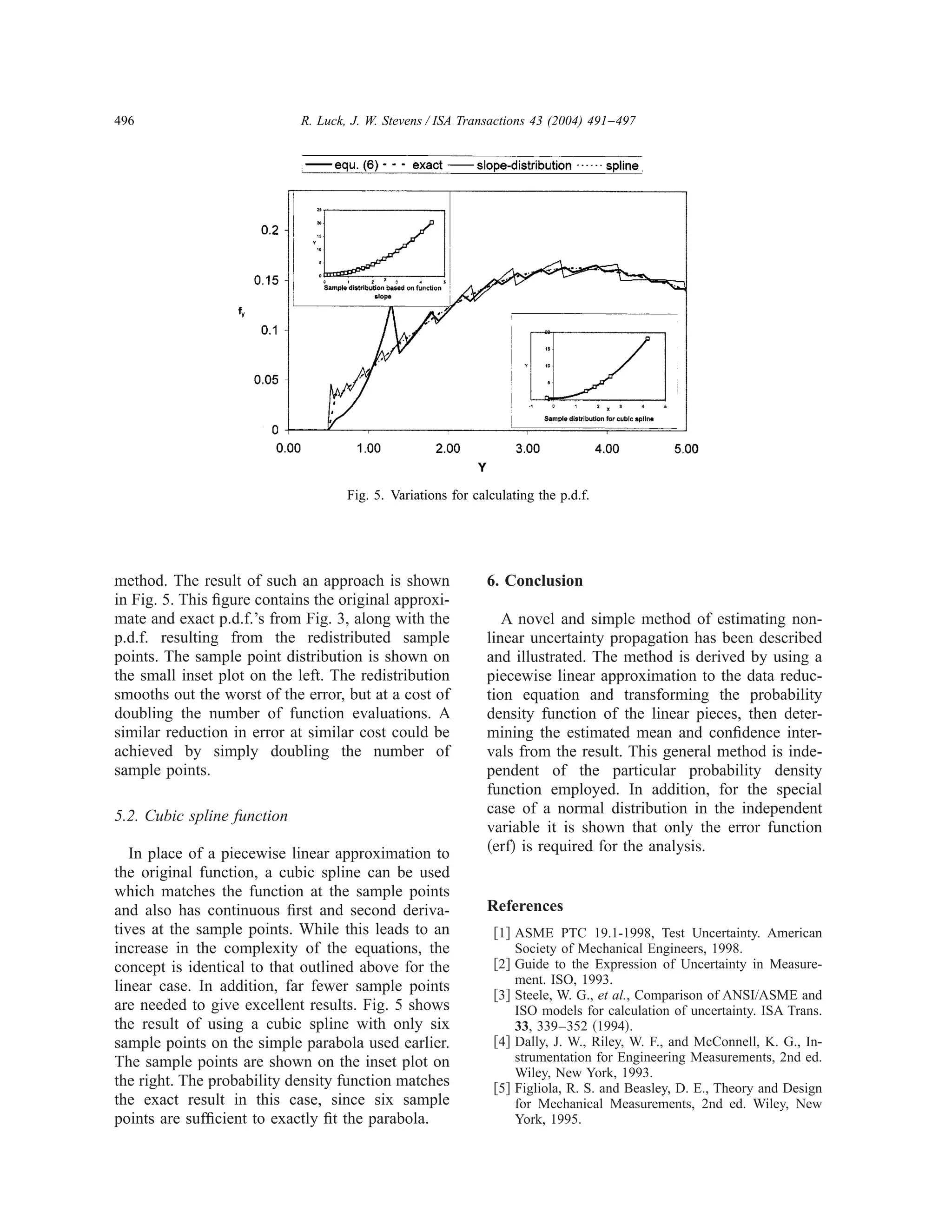
ISA
                                                                                                          TRANSACTIONS®
                                             ISA Transactions 43 ͑2004͒ 491–497


A simple numerical procedure for estimating nonlinear uncertainty
                         propagation
                                                        R. Luck*
     Mechanical Engineering Department, Mississippi State University, Mail Stop 9552, 210 Carpenter Building, P.O. Box ME,
                                              Mississippi State, MS 39762, USA

                                                    J. W. Stevens†
    Dept. of Mechanical and Aerospace Engineering, University of Colorado at Colorado Springs, 1420 Austin Bluffs Parkway,
                          Campus Box UH3, P.O. Box 7150, Colorado Springs, CO 80933-7150, USA
                                   ͑Received 25 September 2003; accepted 15 March 2004͒


Abstract
   Accurately determining the effect of the propagation of uncertainty in nonlinear applications can be awkward and
difficult. The Monte Carlo approach requires statistically significant numbers of function evaluations ͑typically 105 or
more͒ and analytical methods are intractable for all but the simplest cases. This paper derives and demonstrates a
method to estimate the propagation of uncertainty in nonlinear cases by representing the function in a piecewise fashion
with straight line segments. The probability density function of the result can be calculated from the transformation of
the line segments. The mean and confidence intervals of the result can then be calculated from the probability density
function. For the special case of a normal distribution in the independent variable, calculation of the mean and
confidence intervals requires evaluation of only the error function ͑erf͒. A simple example is presented to demonstrate
the technique. Variations on the basic approach are presented and discussed. © 2004 ISA—The Instrumentation,
Systems, and Automation Society.

Keywords: Uncertainty; Nonlinear


1. Introduction                                                   are based on an assumption of linear behavior for
                                                                  small perturbations in the measured variables. Un-
  One element of experimental uncertainty analy-                  certainty analysis for larger perturbations normally
sis deals with the manner in which uncertainty in                 must return to statistical methods.
measurements propagates into a final result. The                     Highly nonlinear functions are not uncommon
validity of the uncertainty estimate of the result                in engineering analyses. For example, near reso-
rests on both the validity of the measurement un-                 nance, the magnitude of the displacement of a
certainties and the method of propagation of those                mass-spring damper is very sensitive to errors in
uncertainties through the analysis equation. Most                 the frequency. Even relatively good experimental
approaches to engineering uncertainty propagation                 frequency resolution can result in nonlinear effects
                                                                  in determining the propagation of uncertainty to
  *Tel.: ͑662͒ 325-7307; fax: ͑662͒ 325-7223. E-mail ad-          other quantities of interest. Another example can
dress: luck@me.msstate.edu                                        be found in the highly nonlinear property relation-
  †
    Corresponding author. Tel.: ͑719͒ 262-3581; fax: ͑719͒        ships for most fluids close to the critical point.
262-3042. E-mail address: JStevens@eas.uccs.edu                   Measurements of such quantities as temperature,

0019-0578/2004/$ - see front matter © 2004 ISA—The Instrumentation, Systems, and Automation Society.
492                          R. Luck, J. W. Stevens / ISA Transactions 43 (2004) 491–497


pressure, and density are commonly used to fix the            and higher terms of the Taylor approximation are
thermodynamic state and to calculate other prop-             not negligible relative to the second term. The
erties such as enthalpy, internal energy, and en-            Taylor series for a function of one variable, R ( x ) ,
tropy. Propagation of uncertainty through such               expanded around x 0 is

                                                                                                               ͯ
calculations can readily lead to nonlinear effects in
the neighborhood of the critical point.                                                               dR
                                                                      R ͑ x ͒ ϷR ͑ x 0 ͒ ϩ                              ͑ xϪx 0 ͒
   Unfortunately, for many engineering applica-                                                       dx           x0
tions, the inversions of the analysis equations re-
quired for a proper analytical approach are either
unwieldy or impossible to obtain. Monte Carlo
computer simulations can yield satisfactory re-
                                                                                        ϩ
                                                                                            1 d 2R
                                                                                            2! dx 2    ͯ   x0
                                                                                                                   ͑ xϪx 0 ͒ 2 ϩ¯ .      ͑1͒

sults, but typically require very large numbers of
                                                             Then, the condition for the linear approximation to
function evaluations. This paper presents a direct
                                                             be valid is
approach to estimate nonlinear uncertainty propa-
gation by using a piecewise linear approximation
to the analysis function and a normal distribution
for the input variable. The approach can be used
                                                                      dR
                                                                      dx   ͯ   x0
                                                                                    ӷ
                                                                                        1 d 2R
                                                                                        2! dx 2   ͯ   x0
                                                                                                           ͑ xϪx 0 ͒


                                                                                                           ͯ
with any function including tabular data. Using the
                                                                                          1 d 3R
normal distribution, only the error function ͑erf͒                                      ϩ                           ͑ xϪx 0 ͒ 2 ϩ¯ .     ͑2͒
needs to be evaluated.                                                                    3! dx 3              x0

                                                             This condition tends to be violated by large higher
2. Background                                                derivatives or large uncertainty ( xϪx 0 ) . Thus
                                                             large uncertainty simply implies that the linear ap-
   The topic of estimation of experimental uncer-            proximation of the truncated Taylor series is inad-
tainty is covered in a wide variety of forums. The           equate to represent the data reduction equation.
American Society of Mechanical Engineers pub-                  An analytical approach for estimating nonlinear
lishes an uncertainty standard as part of the per-           uncertainty propagation is to transform the prob-
formance test codes: ASME PTC 19.1-1998, Test                ability density function ͑p.d.f.͒ of the measured
Uncertainty ͓1͔. The International Organization              variable through the data reduction equation to get
for Standardization ͑ISO͒ also publishes a guide             a probability density function for the result. The
on uncertainty calculation and terminology en-               expected mean and confidence intervals can then
titled ‘‘Guide to the Expression of Uncertainty in           be calculated from the p.d.f. of the result. If x is
Measurement’’ ͓2͔. These two approaches are                  the measured variable, and f x ( x ) is the p.d.f. of
compared by Steele et al. ͓3͔. Most textbooks on             that variable, and yϭh ( x ) is the data reduction
experimental measurements include a section on               equation, then the p.d.f. for the result can be cal-
uncertainty propagation as well ͑for example,                culated by
Refs. ͓4 – 6͔͒. Some textbooks specialize in uncer-
tainty ͓7,8͔. The technical literature also has nu-
merous treatments of uncertainty estimation and
propagation in specific applications ͑for example,
                                                                         f y ͑ y ͒ ϭ f x „h Ϫ1 ͑ y ͒ …               ͯ   dh Ϫ1 ͑ y ͒
                                                                                                                            dy      ͯ.   ͑3͒

Refs. ͓9–12͔͒.                                               While this works easily for simple functions, the
   While estimation of measurement uncertainty is            inversion of the analysis equation can become
treated in great detail in these references, the             very awkward or impossible for complicated func-
propagation of measurement uncertainty in data               tions or tabular data.
reduction or data analysis equations is invariably              The approach demonstrated in this paper is to
handled by a truncated Taylor expansion. This ap-            approximate the analysis function with a series of
proach to propagation assumes that the uncertainty           straight line segments. The transformation for the
in a measured variable is not too large for the data         line segments is straightforward and an approxi-
reduction equation to be represented well locally            mate p.d.f. for the dependent variable can be con-
by a straight line. More precisely in this context,          structed. From that p.d.f., an estimate of the mean
‘‘large’’ perturbations simply means that the third          and confidence intervals can be obtained. For the
R. Luck, J. W. Stevens / ISA Transactions 43 (2004) 491–497                                                          493


                                                              tities of primary interest. The mean can be ex-
                                                              pressed in terms of the probability density func-
                                                              tion by

                                                                                      ␮ yϭ       ͵    ϱ

                                                                                                      Ϫϱ
                                                                                                           y f y dy.                               ͑7͒

                                                              For an N segment, piecewise linear approximation
                                                              to the function this becomes

                                                                                       ͵
                                                                               NϪ1
                                                                                           x kϩ1
                                                                        ␮ yϭ ͚                        ͑ a k ␰ ϩb k ͒ f x ͑ ␰ ͒ d ␰
                                                                               kϭ0      xk


                                                                                           ͵
                                                                               NϪ1
                                                                                                 x kϩ1
                                                                           ϭ   ͚
                                                                               kϭ0
                                                                                      ak
                                                                                                 xk
                                                                                                           ͑ ␰ ͒ f x͑ ␰ ͒ d ␰
        Fig. 1. Nomenclature of line segments.
                                                                               ϩb k   ͵ xk
                                                                                           x kϩ1
                                                                                                      f x͑ ␰ ͒ d ␰ ,                               ͑8͒
special case of a normal distribution in the mea-
sured variable, the mean and confidence intervals              where ␰ is the dummy variable of integration be-
will be shown to depend only on evaluation of the             tween limits x k and x kϩ1 .
error function ͑erf͒.                                            Using integration by parts on the first term and
                                                              using the cumulative distribution function defined
3. Development                                                as

  Consider a linear function of the form: yϭax
ϩb, with a probability density function on the
                                                                                F x͑ x ͒ ϭ        ͵    x

                                                                                                       Ϫϱ
                                                                                                               f x͑ ␰ ͒ d ␰                        ͑9͒

independent variable of f x ( x ) . Then from Eq. ͑3͒,        then Eq. ͑8͒ can be written
the probability density function of the dependent

                                                                                  ͫ                                 ͵                          ͬ
                                                                        NϪ1
variable is given by                                                                                                    x kϩ1
                                                                  ␮ y ϭ ͚ a k ␰ F x ͑ ␰ ͒ ͉ x kϩ1 Ϫ
                                                                                            x
                                                                                                                                F x͑ ␰ ͒ d ␰
               f y͑ y ͒ϭ
                          1
                         ͉a͉ ͩ ͪ
                             fx
                                yϪb
                                 a
                                    .               ͑4͒
                                                                         kϭ0

                                                                                         x
                                                                        ϩb k F x ͑ ␰ ͒ ͉ x kϩ1 .
                                                                                                           k          xk


                                                                                                                                               ͑10͒
                                                                                             k
Over a range of interest, an analysis function or
tabular data may be approximated by a series of               3.2. Confidence interval
line segments of arbitrary length ͑see Fig. 1͒:
            yϭa k xϩb k ,   x k ϽxϽx kϩ1 .          ͑5͒         Approximate confidence intervals can be taken
                                                              directly from the cumulative distribution function
For each segment, the probability density function            of the dependent variable. For the N-segment
of the dependent variable is given by the piece-              piecewise linear approximation this is
wise version of Eq. ͑4͒:
                                                                                       ͵                            ͩ ͪ
                                                                                  P
                                                                                                               ␭Ϫb k
                     ͩ ͪ
                                                                                             y kϩ1        1
                 1     yϪb k                                          F y͑ y ͒ϭ ͚                            f       d␭, ͑11͒
     f y͑ y ͒ϭ       f       ,    y k ϽyϽy kϩ1 . ͑6͒                            kϭ0         yk         ͉ a k͉ x a k
               ͉ a k͉ x a k
                                                              where P is the interval containing the argument of
3.1. Mean                                                     the cumulative distribution function.

  Normally, the probability density function tends            3.3. Normal distribution
to be of lesser direct interest for the purposes of
engineering uncertainty analysis. Instead, the                  Eqs. ͑10͒ and ͑11͒ are valid for any probability
mean and confidence intervals are often the quan-              density function of the independent variable. For
494                                      R. Luck, J. W. Stevens / ISA Transactions 43 (2004) 491–497


the special ͑and most common͒ case of a normal
distribution, a further simplification for the evalu-
ation of Eqs. ͑10͒ and ͑11͒ is possible. However, it
must be emphasized that Eqs. ͑10͒ and ͑11͒ are
general in nature and are applicable to any prob-
ability density function. The additional steps de-
scribed below render the evaluation of Eqs. ͑10͒
and ͑11͒ very convenient for a single special case;
that of a normal distribution.
   For a normal distribution with mean ␮ x and
standard deviation ␴, the probability density func-
tion can be written                                                                         Fig. 2. Example function with data samples.

                             1                             2
                                                               /2␴ 2
             f x͑ z ͒ ϭ               e Ϫ ͑ zϪ ␮ x ͒                   .       ͑12͒   4. Simple example
                          ␴ ͱ2 ␲
                                                                                         A simple example will be used to illustrate this
The corresponding cumulative distribution func-
                                                                                      approach to uncertainty estimation. This rather
tion for a normal distribution is
                                                                                      trivial one-dimensional mathematical function was

      F͑ x ͒ϭ
      ˆ         ͵Ϫϱ
                    x
                    f
                                   1 1
                    ˆ x ͑ ␰ ͒ d ␰ ϭ ϩ erf
                                   2 2
                                          xϪ ␮ x
                                           ␴&
                                                 ,             ͩ ͪ                    chosen so that the exact analytical solution is
                                                                                      available for comparison in order to better illus-
                                                                                      trate the method. While many real one-
                                                  ͑13͒                                dimensional uncertainty problems exist ͑thermo-
where erf is the error function defined as                                             couple voltage-temperature curves, ideal gas
                                                                                      pressure-temperature relation at fixed volume,

                    erf͑ x ͒ ϭ
                                 2
                                 ͱ␲
                                    ͵e   0
                                            x
                                                    Ϫt 2
                                                           dt.                 ͑14͒
                                                                                      etc.͒, few are represented by such a conveniently
                                                                                      simple function. Hence this mathematical function
                                                                                      was chosen primarily for clarity in illustration.
After some algebra it can be shown that for the                                          Assume that the data reduction equation is a pa-
normal distribution ͓Eq. ͑12͔͒,                                                       rabola,


  ͵                                                      ␮x                                               yϭx 2 ϩ0.5,                     ͑18͒
       F x͑ ␰ ͒ d ␰ ϭ ͑ ␰ Ϫ ␮ x ͒ F x͑ ␰ ͒ ϩ ␴ f x͑ ␰ ͒ ϩ .
       ˆ                          ˆ                         2ˆ
                                                         2                            and that the uncertainty is to be evaluated around
                                                          ͑15͒                        xϭ2. The independent variable is distributed nor-
With this result, Eq. ͑10͒ can be expressed                                           mally with a standard deviation ␴ of 0.65.
                                                                                         Fig. 2 shows the parabola ͓Eq. ͑18͔͒ with 21

                        ͯͫ ͩ                           ͪ                   ͬ
            NϪ1
                                                     1                                data samples spaced, for this example, at even in-
      ␮ y ϭ ͚ a k ␮ x F x͑ ␰ ͒ Ϫ
      ˆ               ˆ                                Ϫ ␴ 2 ˆ x͑ ␰ ͒
                                                             f                        tervals of probability in a normal distribution. The
            kϭ0                                      2
                                                                                      sample spacing is not critical to the analysis.

            ϩb k F x ͑ ␰ ͒
                 ˆ         ͯ ␰ ϭx kϩ1


                             ␰ ϭx k
                                        .                                      ͑16͒
                                                                                         Fig. 3 shows the approximate probability den-
                                                                                      sity function for y calculated according to Eq. ͑6͒.
                                                                                      For comparison, the dashed line in Fig. 3 shows
                                                                                      the exact probability density function from Eq. ͑4͒
For evaluating the confidence interval ͓Eq. ͑11͔͒, it
                                                                                      which is easy to calculate for this simple case of a
can be shown that for the special case of the nor-
                                                                                      parabola. The triangles in Fig. 3 shows the results
mal distribution,
                                                                                      of the probability density function calculated from

        ͵ ˆf ͩ yϪb ͪ dyϭaͫ F ͩ yϪb ͪ Ϫ 2 ͬ .
             x
                a
                           ˆ
                                a
                                       1
                                                x                              ͑17͒
                                                                                      a Monte Carlo analysis with one million function
                                                                                      evaluations. By comparison, the approximate
                                                                                      probability density function calculated from Eq.
Thus, for this special case, both the mean and con-                                   ͑6͒ required only 21 function evaluations.
fidence interval can be evaluated using only the                                          The mean for y, ␮ y , calculated from Eq. ͑16͒
error function.                                                                       with the 21 data points shown in Fig. 2, is 4.9122
R. Luck, J. W. Stevens / ISA Transactions 43 (2004) 491–497                     495


                                                                solution. Also as expected, the error in the first-
                                                                order analysis increases rapidly with the level of
                                                                uncertainty in the independent variable, rising
                                                                from less than 0.5% at ␴ ϭ0.15 to nearly 17% at
                                                                ␴ ϭ0.95. This increase is approximately propor-
                                                                tional to the square of the standard deviation for
                                                                this particular case. The error from Eq. ͑16͒, on
                                                                the other hand, decreases slightly with increasing
                                                                independent variable uncertainty and is less than
                                                                0.3% over the range shown in Fig. 4.
                                                                   Using Eq. ͑11͒ with the simplification of Eq.
                                                                ͑17͒, the 5% and 95% confidence limits are calcu-
          Fig. 3. Probability density function.
                                                                lated at 1.382 and 9.987, respectively for the case
                                                                of ␴ ϭ0.65. For this simple case, the confidence
while the exact mean would be 4.9225, or a dif-                 limits calculated from the linear analysis are quite
ference of 0.2%. For comparison, the mean value                 close ͑1.366 and 9.92, respectively͒, but in gen-
calculated from a one-million-point Monte Carlo                 eral, they may differ significantly due to the non-
analysis is 4.9226, a difference of 0.002%. For a               linearity. The differences in confidence intervals
simple first-order uncertainty analysis the mean                 between those calculated by Eq. ͑11͒ and those
would be 4.5, or a difference of 8.6% from the                  from a first-order analysis increase with increasing
exact result. Thus, even on this simple equation                standard deviation in a manner similar to ␮ y , but
with relatively gentle curvature, there is a signifi-            with smaller magnitude.
cant effect of the nonlinearities on the uncertainty
propagation.                                                    5. Variations
  This effect is explored more fully in Fig. 4
where the percent error in ␮ y with respect to the                While one of the most attractive features of the
exact answer is plotted as a function of the stan-              method outlined above lies in its simplicity, the
dard deviation in the independent variable x. The               overall efficiency and accuracy of the method can
standard deviation is representative of the uncer-              be improved slightly at the expense of somewhat
tainty in the independent variable. The errors for              greater complexity. Two such variations are ex-
the one-million-point Monte Carlo analysis and                  plained below.
for Eq. ͑16͒ are plotted with the left vertical scale,
while the error in the first-order analysis is plotted           5.1. Sample distribution
with the right vertical scale.
  As would be expected, the one-million-point                      The probability density function from Eq. ͑6͒
Monte Carlo analysis is nearly exact, with very                 shown in Fig. 3 exhibits increasing instability as x
small random errors around the exact analytical                 approaches zero. This is because the transforma-
                                                                tion of the linear pieces becomes undefined at zero
                                                                slope. Furthermore, as the slope gets small, the
                                                                inverse of the slope ͓see Eq. ͑4͔͒ gets large, and
                                                                small changes in the slope are amplified. Thus
                                                                there are large changes between each piece of the
                                                                approximation. A possible improvement would be
                                                                for the sample points to be distributed more
                                                                closely in areas where the function slope is small.
                                                                For a fixed number of total sample points, this can
                                                                be accomplished relatively easily, but at the cost
                                                                of making two passes of function evaluations: one
                                                                to calculate the slopes, and another to redistribute
                                                                the sample points. This results in approximately
      Fig. 4. Error in calculated mean values ␮ y .             twice as many function evaluations as the original
496                          R. Luck, J. W. Stevens / ISA Transactions 43 (2004) 491–497


                                     Fig. 5. Variations for calculating the p.d.f.


method. The result of such an approach is shown               6. Conclusion
in Fig. 5. This figure contains the original approxi-
mate and exact p.d.f.’s from Fig. 3, along with the              A novel and simple method of estimating non-
p.d.f. resulting from the redistributed sample                linear uncertainty propagation has been described
points. The sample point distribution is shown on             and illustrated. The method is derived by using a
the small inset plot on the left. The redistribution          piecewise linear approximation to the data reduc-
smooths out the worst of the error, but at a cost of          tion equation and transforming the probability
doubling the number of function evaluations. A                density function of the linear pieces, then deter-
similar reduction in error at similar cost could be           mining the estimated mean and confidence inter-
achieved by simply doubling the number of                     vals from the result. This general method is inde-
sample points.                                                pendent of the particular probability density
                                                              function employed. In addition, for the special
5.2. Cubic spline function                                    case of a normal distribution in the independent
                                                              variable it is shown that only the error function
   In place of a piecewise linear approximation to            ͑erf͒ is required for the analysis.
the original function, a cubic spline can be used
which matches the function at the sample points
and also has continuous first and second deriva-               References
tives at the sample points. While this leads to an              ͓1͔ ASME PTC 19.1-1998, Test Uncertainty. American
increase in the complexity of the equations, the                    Society of Mechanical Engineers, 1998.
concept is identical to that outlined above for the             ͓2͔ Guide to the Expression of Uncertainty in Measure-
                                                                    ment. ISO, 1993.
linear case. In addition, far fewer sample points
                                                                ͓3͔ Steele, W. G., et al., Comparison of ANSI/ASME and
are needed to give excellent results. Fig. 5 shows                  ISO models for calculation of uncertainty. ISA Trans.
the result of using a cubic spline with only six                    33, 339–352 ͑1994͒.
sample points on the simple parabola used earlier.              ͓4͔ Dally, J. W., Riley, W. F., and McConnell, K. G., In-
The sample points are shown on the inset plot on                    strumentation for Engineering Measurements, 2nd ed.
                                                                    Wiley, New York, 1993.
the right. The probability density function matches             ͓5͔ Figliola, R. S. and Beasley, D. E., Theory and Design
the exact result in this case, since six sample                     for Mechanical Measurements, 2nd ed. Wiley, New
points are sufficient to exactly fit the parabola.                    York, 1995.
R. Luck, J. W. Stevens / ISA Transactions 43 (2004) 491–497                             497

͓6͔ Holman, J. P., Experimental Methods for Engineers,          ͓10͔ Kline, S. J. and McClintock, F. A., Describing uncer-
    5th ed. McGraw-Hill, New York, 1989.                             tainties in single sample experiments. Mech. Eng.
͓7͔ Barry, B. A., Engineering Measurements. Wiley, New               ͑Am. Soc. Mech. Eng.͒ 75, 3– 8 ͑1953͒.
    York, 1964.                                                 ͓11͔ Coleman, H. W. and Steele, W. G., Engineering appli-
͓8͔ Coleman, H. W. and Steele, W. G., Experimentation                cation of experimental uncertainty analysis. AIAA J.
    and Uncertainty Analysis for Engineers. Wiley, New               33, 1888 –1896 ͑1995͒.
    York, 1989.                                                 ͓12͔ Wyler, J. S., Estimating the uncertainty of spacial and
͓9͔ Moffat, R. J., Contributions to the theory of a single-          time average measurements. J. Eng. Power October
    sample uncertainty analysis. J. Fluids Eng. 104, 250–            97, 473– 476 ͑1975͒.
    260 ͑1982͒.

A simple numerical procedure for estimating nonlinear uncertainty propagation

  • 1.
    ISA TRANSACTIONS® ISA Transactions 43 ͑2004͒ 491–497 A simple numerical procedure for estimating nonlinear uncertainty propagation R. Luck* Mechanical Engineering Department, Mississippi State University, Mail Stop 9552, 210 Carpenter Building, P.O. Box ME, Mississippi State, MS 39762, USA J. W. Stevens† Dept. of Mechanical and Aerospace Engineering, University of Colorado at Colorado Springs, 1420 Austin Bluffs Parkway, Campus Box UH3, P.O. Box 7150, Colorado Springs, CO 80933-7150, USA ͑Received 25 September 2003; accepted 15 March 2004͒ Abstract Accurately determining the effect of the propagation of uncertainty in nonlinear applications can be awkward and difficult. The Monte Carlo approach requires statistically significant numbers of function evaluations ͑typically 105 or more͒ and analytical methods are intractable for all but the simplest cases. This paper derives and demonstrates a method to estimate the propagation of uncertainty in nonlinear cases by representing the function in a piecewise fashion with straight line segments. The probability density function of the result can be calculated from the transformation of the line segments. The mean and confidence intervals of the result can then be calculated from the probability density function. For the special case of a normal distribution in the independent variable, calculation of the mean and confidence intervals requires evaluation of only the error function ͑erf͒. A simple example is presented to demonstrate the technique. Variations on the basic approach are presented and discussed. © 2004 ISA—The Instrumentation, Systems, and Automation Society. Keywords: Uncertainty; Nonlinear 1. Introduction are based on an assumption of linear behavior for small perturbations in the measured variables. Un- One element of experimental uncertainty analy- certainty analysis for larger perturbations normally sis deals with the manner in which uncertainty in must return to statistical methods. measurements propagates into a final result. The Highly nonlinear functions are not uncommon validity of the uncertainty estimate of the result in engineering analyses. For example, near reso- rests on both the validity of the measurement un- nance, the magnitude of the displacement of a certainties and the method of propagation of those mass-spring damper is very sensitive to errors in uncertainties through the analysis equation. Most the frequency. Even relatively good experimental approaches to engineering uncertainty propagation frequency resolution can result in nonlinear effects in determining the propagation of uncertainty to *Tel.: ͑662͒ 325-7307; fax: ͑662͒ 325-7223. E-mail ad- other quantities of interest. Another example can dress: luck@me.msstate.edu be found in the highly nonlinear property relation- † Corresponding author. Tel.: ͑719͒ 262-3581; fax: ͑719͒ ships for most fluids close to the critical point. 262-3042. E-mail address: JStevens@eas.uccs.edu Measurements of such quantities as temperature, 0019-0578/2004/$ - see front matter © 2004 ISA—The Instrumentation, Systems, and Automation Society.
  • 2.
    492 R. Luck, J. W. Stevens / ISA Transactions 43 (2004) 491–497 pressure, and density are commonly used to fix the and higher terms of the Taylor approximation are thermodynamic state and to calculate other prop- not negligible relative to the second term. The erties such as enthalpy, internal energy, and en- Taylor series for a function of one variable, R ( x ) , tropy. Propagation of uncertainty through such expanded around x 0 is ͯ calculations can readily lead to nonlinear effects in the neighborhood of the critical point. dR R ͑ x ͒ ϷR ͑ x 0 ͒ ϩ ͑ xϪx 0 ͒ Unfortunately, for many engineering applica- dx x0 tions, the inversions of the analysis equations re- quired for a proper analytical approach are either unwieldy or impossible to obtain. Monte Carlo computer simulations can yield satisfactory re- ϩ 1 d 2R 2! dx 2 ͯ x0 ͑ xϪx 0 ͒ 2 ϩ¯ . ͑1͒ sults, but typically require very large numbers of Then, the condition for the linear approximation to function evaluations. This paper presents a direct be valid is approach to estimate nonlinear uncertainty propa- gation by using a piecewise linear approximation to the analysis function and a normal distribution for the input variable. The approach can be used dR dx ͯ x0 ӷ 1 d 2R 2! dx 2 ͯ x0 ͑ xϪx 0 ͒ ͯ with any function including tabular data. Using the 1 d 3R normal distribution, only the error function ͑erf͒ ϩ ͑ xϪx 0 ͒ 2 ϩ¯ . ͑2͒ needs to be evaluated. 3! dx 3 x0 This condition tends to be violated by large higher 2. Background derivatives or large uncertainty ( xϪx 0 ) . Thus large uncertainty simply implies that the linear ap- The topic of estimation of experimental uncer- proximation of the truncated Taylor series is inad- tainty is covered in a wide variety of forums. The equate to represent the data reduction equation. American Society of Mechanical Engineers pub- An analytical approach for estimating nonlinear lishes an uncertainty standard as part of the per- uncertainty propagation is to transform the prob- formance test codes: ASME PTC 19.1-1998, Test ability density function ͑p.d.f.͒ of the measured Uncertainty ͓1͔. The International Organization variable through the data reduction equation to get for Standardization ͑ISO͒ also publishes a guide a probability density function for the result. The on uncertainty calculation and terminology en- expected mean and confidence intervals can then titled ‘‘Guide to the Expression of Uncertainty in be calculated from the p.d.f. of the result. If x is Measurement’’ ͓2͔. These two approaches are the measured variable, and f x ( x ) is the p.d.f. of compared by Steele et al. ͓3͔. Most textbooks on that variable, and yϭh ( x ) is the data reduction experimental measurements include a section on equation, then the p.d.f. for the result can be cal- uncertainty propagation as well ͑for example, culated by Refs. ͓4 – 6͔͒. Some textbooks specialize in uncer- tainty ͓7,8͔. The technical literature also has nu- merous treatments of uncertainty estimation and propagation in specific applications ͑for example, f y ͑ y ͒ ϭ f x „h Ϫ1 ͑ y ͒ … ͯ dh Ϫ1 ͑ y ͒ dy ͯ. ͑3͒ Refs. ͓9–12͔͒. While this works easily for simple functions, the While estimation of measurement uncertainty is inversion of the analysis equation can become treated in great detail in these references, the very awkward or impossible for complicated func- propagation of measurement uncertainty in data tions or tabular data. reduction or data analysis equations is invariably The approach demonstrated in this paper is to handled by a truncated Taylor expansion. This ap- approximate the analysis function with a series of proach to propagation assumes that the uncertainty straight line segments. The transformation for the in a measured variable is not too large for the data line segments is straightforward and an approxi- reduction equation to be represented well locally mate p.d.f. for the dependent variable can be con- by a straight line. More precisely in this context, structed. From that p.d.f., an estimate of the mean ‘‘large’’ perturbations simply means that the third and confidence intervals can be obtained. For the
  • 3.
    R. Luck, J.W. Stevens / ISA Transactions 43 (2004) 491–497 493 tities of primary interest. The mean can be ex- pressed in terms of the probability density func- tion by ␮ yϭ ͵ ϱ Ϫϱ y f y dy. ͑7͒ For an N segment, piecewise linear approximation to the function this becomes ͵ NϪ1 x kϩ1 ␮ yϭ ͚ ͑ a k ␰ ϩb k ͒ f x ͑ ␰ ͒ d ␰ kϭ0 xk ͵ NϪ1 x kϩ1 ϭ ͚ kϭ0 ak xk ͑ ␰ ͒ f x͑ ␰ ͒ d ␰ Fig. 1. Nomenclature of line segments. ϩb k ͵ xk x kϩ1 f x͑ ␰ ͒ d ␰ , ͑8͒ special case of a normal distribution in the mea- sured variable, the mean and confidence intervals where ␰ is the dummy variable of integration be- will be shown to depend only on evaluation of the tween limits x k and x kϩ1 . error function ͑erf͒. Using integration by parts on the first term and using the cumulative distribution function defined 3. Development as Consider a linear function of the form: yϭax ϩb, with a probability density function on the F x͑ x ͒ ϭ ͵ x Ϫϱ f x͑ ␰ ͒ d ␰ ͑9͒ independent variable of f x ( x ) . Then from Eq. ͑3͒, then Eq. ͑8͒ can be written the probability density function of the dependent ͫ ͵ ͬ NϪ1 variable is given by x kϩ1 ␮ y ϭ ͚ a k ␰ F x ͑ ␰ ͒ ͉ x kϩ1 Ϫ x F x͑ ␰ ͒ d ␰ f y͑ y ͒ϭ 1 ͉a͉ ͩ ͪ fx yϪb a . ͑4͒ kϭ0 x ϩb k F x ͑ ␰ ͒ ͉ x kϩ1 . k xk ͑10͒ k Over a range of interest, an analysis function or tabular data may be approximated by a series of 3.2. Confidence interval line segments of arbitrary length ͑see Fig. 1͒: yϭa k xϩb k , x k ϽxϽx kϩ1 . ͑5͒ Approximate confidence intervals can be taken directly from the cumulative distribution function For each segment, the probability density function of the dependent variable. For the N-segment of the dependent variable is given by the piece- piecewise linear approximation this is wise version of Eq. ͑4͒: ͵ ͩ ͪ P ␭Ϫb k ͩ ͪ y kϩ1 1 1 yϪb k F y͑ y ͒ϭ ͚ f d␭, ͑11͒ f y͑ y ͒ϭ f , y k ϽyϽy kϩ1 . ͑6͒ kϭ0 yk ͉ a k͉ x a k ͉ a k͉ x a k where P is the interval containing the argument of 3.1. Mean the cumulative distribution function. Normally, the probability density function tends 3.3. Normal distribution to be of lesser direct interest for the purposes of engineering uncertainty analysis. Instead, the Eqs. ͑10͒ and ͑11͒ are valid for any probability mean and confidence intervals are often the quan- density function of the independent variable. For
  • 4.
    494 R. Luck, J. W. Stevens / ISA Transactions 43 (2004) 491–497 the special ͑and most common͒ case of a normal distribution, a further simplification for the evalu- ation of Eqs. ͑10͒ and ͑11͒ is possible. However, it must be emphasized that Eqs. ͑10͒ and ͑11͒ are general in nature and are applicable to any prob- ability density function. The additional steps de- scribed below render the evaluation of Eqs. ͑10͒ and ͑11͒ very convenient for a single special case; that of a normal distribution. For a normal distribution with mean ␮ x and standard deviation ␴, the probability density func- tion can be written Fig. 2. Example function with data samples. 1 2 /2␴ 2 f x͑ z ͒ ϭ e Ϫ ͑ zϪ ␮ x ͒ . ͑12͒ 4. Simple example ␴ ͱ2 ␲ A simple example will be used to illustrate this The corresponding cumulative distribution func- approach to uncertainty estimation. This rather tion for a normal distribution is trivial one-dimensional mathematical function was F͑ x ͒ϭ ˆ ͵Ϫϱ x f 1 1 ˆ x ͑ ␰ ͒ d ␰ ϭ ϩ erf 2 2 xϪ ␮ x ␴& , ͩ ͪ chosen so that the exact analytical solution is available for comparison in order to better illus- trate the method. While many real one- ͑13͒ dimensional uncertainty problems exist ͑thermo- where erf is the error function defined as couple voltage-temperature curves, ideal gas pressure-temperature relation at fixed volume, erf͑ x ͒ ϭ 2 ͱ␲ ͵e 0 x Ϫt 2 dt. ͑14͒ etc.͒, few are represented by such a conveniently simple function. Hence this mathematical function was chosen primarily for clarity in illustration. After some algebra it can be shown that for the Assume that the data reduction equation is a pa- normal distribution ͓Eq. ͑12͔͒, rabola, ͵ ␮x yϭx 2 ϩ0.5, ͑18͒ F x͑ ␰ ͒ d ␰ ϭ ͑ ␰ Ϫ ␮ x ͒ F x͑ ␰ ͒ ϩ ␴ f x͑ ␰ ͒ ϩ . ˆ ˆ 2ˆ 2 and that the uncertainty is to be evaluated around ͑15͒ xϭ2. The independent variable is distributed nor- With this result, Eq. ͑10͒ can be expressed mally with a standard deviation ␴ of 0.65. Fig. 2 shows the parabola ͓Eq. ͑18͔͒ with 21 ͯͫ ͩ ͪ ͬ NϪ1 1 data samples spaced, for this example, at even in- ␮ y ϭ ͚ a k ␮ x F x͑ ␰ ͒ Ϫ ˆ ˆ Ϫ ␴ 2 ˆ x͑ ␰ ͒ f tervals of probability in a normal distribution. The kϭ0 2 sample spacing is not critical to the analysis. ϩb k F x ͑ ␰ ͒ ˆ ͯ ␰ ϭx kϩ1 ␰ ϭx k . ͑16͒ Fig. 3 shows the approximate probability den- sity function for y calculated according to Eq. ͑6͒. For comparison, the dashed line in Fig. 3 shows the exact probability density function from Eq. ͑4͒ For evaluating the confidence interval ͓Eq. ͑11͔͒, it which is easy to calculate for this simple case of a can be shown that for the special case of the nor- parabola. The triangles in Fig. 3 shows the results mal distribution, of the probability density function calculated from ͵ ˆf ͩ yϪb ͪ dyϭaͫ F ͩ yϪb ͪ Ϫ 2 ͬ . x a ˆ a 1 x ͑17͒ a Monte Carlo analysis with one million function evaluations. By comparison, the approximate probability density function calculated from Eq. Thus, for this special case, both the mean and con- ͑6͒ required only 21 function evaluations. fidence interval can be evaluated using only the The mean for y, ␮ y , calculated from Eq. ͑16͒ error function. with the 21 data points shown in Fig. 2, is 4.9122
  • 5.
    R. Luck, J.W. Stevens / ISA Transactions 43 (2004) 491–497 495 solution. Also as expected, the error in the first- order analysis increases rapidly with the level of uncertainty in the independent variable, rising from less than 0.5% at ␴ ϭ0.15 to nearly 17% at ␴ ϭ0.95. This increase is approximately propor- tional to the square of the standard deviation for this particular case. The error from Eq. ͑16͒, on the other hand, decreases slightly with increasing independent variable uncertainty and is less than 0.3% over the range shown in Fig. 4. Using Eq. ͑11͒ with the simplification of Eq. ͑17͒, the 5% and 95% confidence limits are calcu- Fig. 3. Probability density function. lated at 1.382 and 9.987, respectively for the case of ␴ ϭ0.65. For this simple case, the confidence while the exact mean would be 4.9225, or a dif- limits calculated from the linear analysis are quite ference of 0.2%. For comparison, the mean value close ͑1.366 and 9.92, respectively͒, but in gen- calculated from a one-million-point Monte Carlo eral, they may differ significantly due to the non- analysis is 4.9226, a difference of 0.002%. For a linearity. The differences in confidence intervals simple first-order uncertainty analysis the mean between those calculated by Eq. ͑11͒ and those would be 4.5, or a difference of 8.6% from the from a first-order analysis increase with increasing exact result. Thus, even on this simple equation standard deviation in a manner similar to ␮ y , but with relatively gentle curvature, there is a signifi- with smaller magnitude. cant effect of the nonlinearities on the uncertainty propagation. 5. Variations This effect is explored more fully in Fig. 4 where the percent error in ␮ y with respect to the While one of the most attractive features of the exact answer is plotted as a function of the stan- method outlined above lies in its simplicity, the dard deviation in the independent variable x. The overall efficiency and accuracy of the method can standard deviation is representative of the uncer- be improved slightly at the expense of somewhat tainty in the independent variable. The errors for greater complexity. Two such variations are ex- the one-million-point Monte Carlo analysis and plained below. for Eq. ͑16͒ are plotted with the left vertical scale, while the error in the first-order analysis is plotted 5.1. Sample distribution with the right vertical scale. As would be expected, the one-million-point The probability density function from Eq. ͑6͒ Monte Carlo analysis is nearly exact, with very shown in Fig. 3 exhibits increasing instability as x small random errors around the exact analytical approaches zero. This is because the transforma- tion of the linear pieces becomes undefined at zero slope. Furthermore, as the slope gets small, the inverse of the slope ͓see Eq. ͑4͔͒ gets large, and small changes in the slope are amplified. Thus there are large changes between each piece of the approximation. A possible improvement would be for the sample points to be distributed more closely in areas where the function slope is small. For a fixed number of total sample points, this can be accomplished relatively easily, but at the cost of making two passes of function evaluations: one to calculate the slopes, and another to redistribute the sample points. This results in approximately Fig. 4. Error in calculated mean values ␮ y . twice as many function evaluations as the original
  • 6.
    496 R. Luck, J. W. Stevens / ISA Transactions 43 (2004) 491–497 Fig. 5. Variations for calculating the p.d.f. method. The result of such an approach is shown 6. Conclusion in Fig. 5. This figure contains the original approxi- mate and exact p.d.f.’s from Fig. 3, along with the A novel and simple method of estimating non- p.d.f. resulting from the redistributed sample linear uncertainty propagation has been described points. The sample point distribution is shown on and illustrated. The method is derived by using a the small inset plot on the left. The redistribution piecewise linear approximation to the data reduc- smooths out the worst of the error, but at a cost of tion equation and transforming the probability doubling the number of function evaluations. A density function of the linear pieces, then deter- similar reduction in error at similar cost could be mining the estimated mean and confidence inter- achieved by simply doubling the number of vals from the result. This general method is inde- sample points. pendent of the particular probability density function employed. In addition, for the special 5.2. Cubic spline function case of a normal distribution in the independent variable it is shown that only the error function In place of a piecewise linear approximation to ͑erf͒ is required for the analysis. the original function, a cubic spline can be used which matches the function at the sample points and also has continuous first and second deriva- References tives at the sample points. While this leads to an ͓1͔ ASME PTC 19.1-1998, Test Uncertainty. American increase in the complexity of the equations, the Society of Mechanical Engineers, 1998. concept is identical to that outlined above for the ͓2͔ Guide to the Expression of Uncertainty in Measure- ment. ISO, 1993. linear case. In addition, far fewer sample points ͓3͔ Steele, W. G., et al., Comparison of ANSI/ASME and are needed to give excellent results. Fig. 5 shows ISO models for calculation of uncertainty. ISA Trans. the result of using a cubic spline with only six 33, 339–352 ͑1994͒. sample points on the simple parabola used earlier. ͓4͔ Dally, J. W., Riley, W. F., and McConnell, K. G., In- The sample points are shown on the inset plot on strumentation for Engineering Measurements, 2nd ed. Wiley, New York, 1993. the right. The probability density function matches ͓5͔ Figliola, R. S. and Beasley, D. E., Theory and Design the exact result in this case, since six sample for Mechanical Measurements, 2nd ed. Wiley, New points are sufficient to exactly fit the parabola. York, 1995.
  • 7.
    R. Luck, J.W. Stevens / ISA Transactions 43 (2004) 491–497 497 ͓6͔ Holman, J. P., Experimental Methods for Engineers, ͓10͔ Kline, S. J. and McClintock, F. A., Describing uncer- 5th ed. McGraw-Hill, New York, 1989. tainties in single sample experiments. Mech. Eng. ͓7͔ Barry, B. A., Engineering Measurements. Wiley, New ͑Am. Soc. Mech. Eng.͒ 75, 3– 8 ͑1953͒. York, 1964. ͓11͔ Coleman, H. W. and Steele, W. G., Engineering appli- ͓8͔ Coleman, H. W. and Steele, W. G., Experimentation cation of experimental uncertainty analysis. AIAA J. and Uncertainty Analysis for Engineers. Wiley, New 33, 1888 –1896 ͑1995͒. York, 1989. ͓12͔ Wyler, J. S., Estimating the uncertainty of spacial and ͓9͔ Moffat, R. J., Contributions to the theory of a single- time average measurements. J. Eng. Power October sample uncertainty analysis. J. Fluids Eng. 104, 250– 97, 473– 476 ͑1975͒. 260 ͑1982͒.