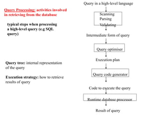
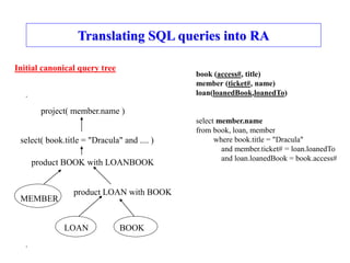
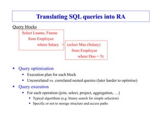
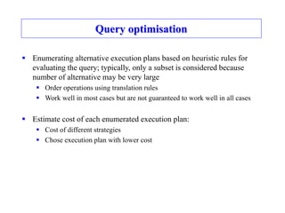
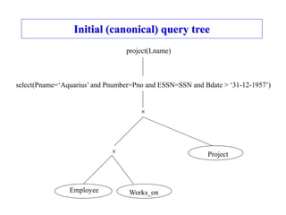
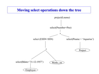
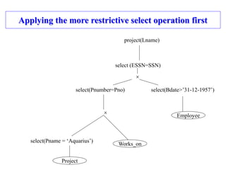
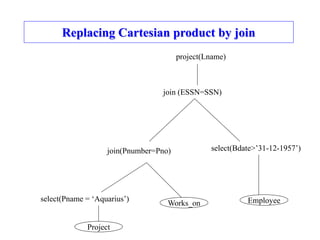
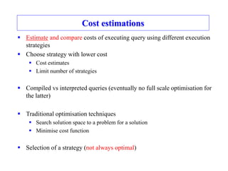
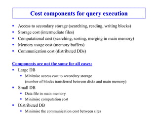
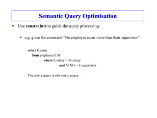
The document discusses query processing and optimization. It describes the typical steps in processing a high-level query like SQL, which are translating the query into an internal representation, optimizing the query execution plan, and executing the plan. The key aspects of optimization are enumerating alternative execution plans using translation rules, estimating the cost of each plan, and choosing the lowest cost plan.

1. Query processing and optimisation
Query processing: The steps
Translating SQL queries into RA
Query execution
Query optimisation
Examples
Translation rules
Cost estimations
Semantic optimisation

2. Query in a high-level language
Scanning
Parsing
Validating
Intermediate form of query
Execution plan
Code to execute the query
Runtime database processor
Result of query
Query code generator
Query optimiser
Query Processing: activities involved
in retrieving from the database
typical steps when processing
a high-level query (e.g SQL
query)
Query tree: internal representation
of the query
Execution strategy: how to retrieve
results of query

3. project( member.name )
select( book.title = "Dracula" and .... )
product BOOK with LOANBOOK
BOOK
product LOAN with BOOK
LOAN
MEMBER
book (access#, title)
member (ticket#, name)
loan(loanedBook,loanedTo)
select member.name
from book, loan, member
where book.title = "Dracula"
and member.ticket# = loan.loanedTo
and loan.loanedBook = book.access#
Translating SQL queries into RA
Initial canonical query tree

4. Translating SQL queries into RA
Query blocks
Select Lname, Fname
from Employee
where Salary > (select Max (Salary)
from Employee
where Dno = 5)
 Query optimisation
 Execution plan for each block
 Uncorrelated vs. correlated nested queries (later harder to optimise)
 Query execution
 For each operation (join, select, project, aggregation, …)
 Typical algorithms (e.g. binary search for simple selection)
 Specific or not to storage structure and access paths

5. project( member.name )
select( book.title = "Dracula" and .... )
product BOOK with LOANBOOK
BOOK
product LOAN with BOOK
LOAN
MEMBER
(1 record)
(30,000,000 records)
(300,000 records)
(1,000 records)
(300 records)
(100 records)
project( member.name )
product MEMBER with LOANDRACULA
product LOAN with DRACULA
LOAN
(300 records)
(300 records)
BOOK (1,000 records)
MEMBER
(100 records)
select( book.title = "Dracula" )
(1 record)
(1 record)
select( member.ticket# = loan.loanedTo)
(100 records)
select( book.access# = loan.loanedBook)
(1 record)
book (access#, title)
member (ticket#, name)
select member.name loan(loanedBook,loanedTo)
from book, loan, member
where book.title = "Dracula"
and member.ticket# = loan.loanedTo
and loan.loanedBook = book.access#

6. Query optimisation
 Enumerating alternative execution plans based on heuristic rules for
evaluating the query; typically, only a subset is considered because
number of alternative may be very large
 Order operations using translation rules
 Work well in most cases but are not guaranteed to work well in all cases
 Estimate cost of each enumerated execution plan:
 Cost of different strategies
 Chose execution plan with lower cost

7. Heuristic rules
initial query tree final query tree
rules of equivalence among
RA expressions
optimise into equivalent best query
query tree (reasonably efficient strategy)

8. Example
Select Lname
from Employee, Works_on, Project
where Pname = ‘Aquarius’ and
Pnumber = Pno and
ESSN=SSN and
Bdate > ‘31-12-1957’;

9. Initial (canonical) query tree
Employee Works_on
Project


select(Pname=‘Aquarius’ and Pnumber=Pno and ESSN=SSN and Bdate > ‘31-12-1957’)
project(Lname)

10. Moving select operations down the tree
Employee
Works_on
Project
select(Bdate>’31-12-1957’)

select (ESSN=SSN) select(Pname = ‘Aquarius’)
select(Pnumber=Pno)
project(Lname)


11. Applying the more restrictive select operation first
Project
Works_on
Employee
select(Bdate>’31-12-1957’)

select (ESSN=SSN)
select(Pname = ‘Aquarius’)
select(Pnumber=Pno)
project(Lname)


12. Replacing Cartesian product by join
Project
Works_on Employee
select(Bdate>’31-12-1957’)
join (ESSN=SSN)
select(Pname = ‘Aquarius’)
join(Pnumber=Pno)
project(Lname)

13. Moving project down the tree
Project
Works_on
Employee
select(Bdate>’31-12-1957’)
project(ESSN,Pno)
select(Pname = ‘Aquarius’)
join(Pnumber=Pno)
project(Pnumber)
project(SSN,Lname)
project(ESSN)
join(ESSN=SSN)
project(Lname)

14. Translation rules (Examples)
 Cascade of select
select (R, c1 and c2 and c3)  select (select (select (R,c1), c2), c3)
 Commutativity of select
select (select (R, c1), c2)  select (select (R, c2), c1)
 Cascade of project
project (project (project (R, A3), A2), A1)  project (R, A1)
where A3  A2  A1

15. Translation rules (Examples)
 Commuting select with join
 select (join (R,S), c)  join (select (R,c), S)
when c applies to R only
 select (join (R,S), c1 and c2)  join (select (R,c1), select (S,c2))
when c1 applies to R
when c2 applies to S
 Commuting select with , , and -
select (R  S, c)  select (R,c)  select (S,c)

16. Rules
Apply first operations that reduce size of intermediary results
1. perform as early as possible select and project
(move down the tree the select and project)
2. execute first most restrictive join and select
reorder leaf nodes
avoid Cartesian product
adjust rest of tree accordingly

17. Cost estimations
 Estimate and compare costs of executing query using different execution
strategies
 Choose strategy with lower cost
 Cost estimates
 Limit number of strategies
 Compiled vs interpreted queries (eventually no full scale optimisation for
the latter)
 Traditional optimisation techniques
 Search solution space to a problem for a solution
 Minimise cost function
 Selection of a strategy (not always optimal)

18. Cost components for query execution
 Access to secondary storage (searching, reading, writing blocks)
 Storage cost (intermediate files)
 Computational cost (searching, sorting, merging in main memory)
 Memory usage cost (memory buffers)
 Communication cost (distributed DBs)
Components are not the same for all cases:
 Large DB
 Minimise access cost to secondary storage
(number of blocks transferred between disks and main memory)
 Small DB
 Data file in main memory
 Minimise computation cost
 Distributed DB
 Minimise the communication cost between sites

19. Semantic Query Optimisation
 Use constraints to guide the query processing:
 e.g. given the constraint “No employee earns more than their supervisor”
select E.name
from employee E M
where E.salary > M.salary
and M.NI# = E.supervisor
The above query is obviously empty.