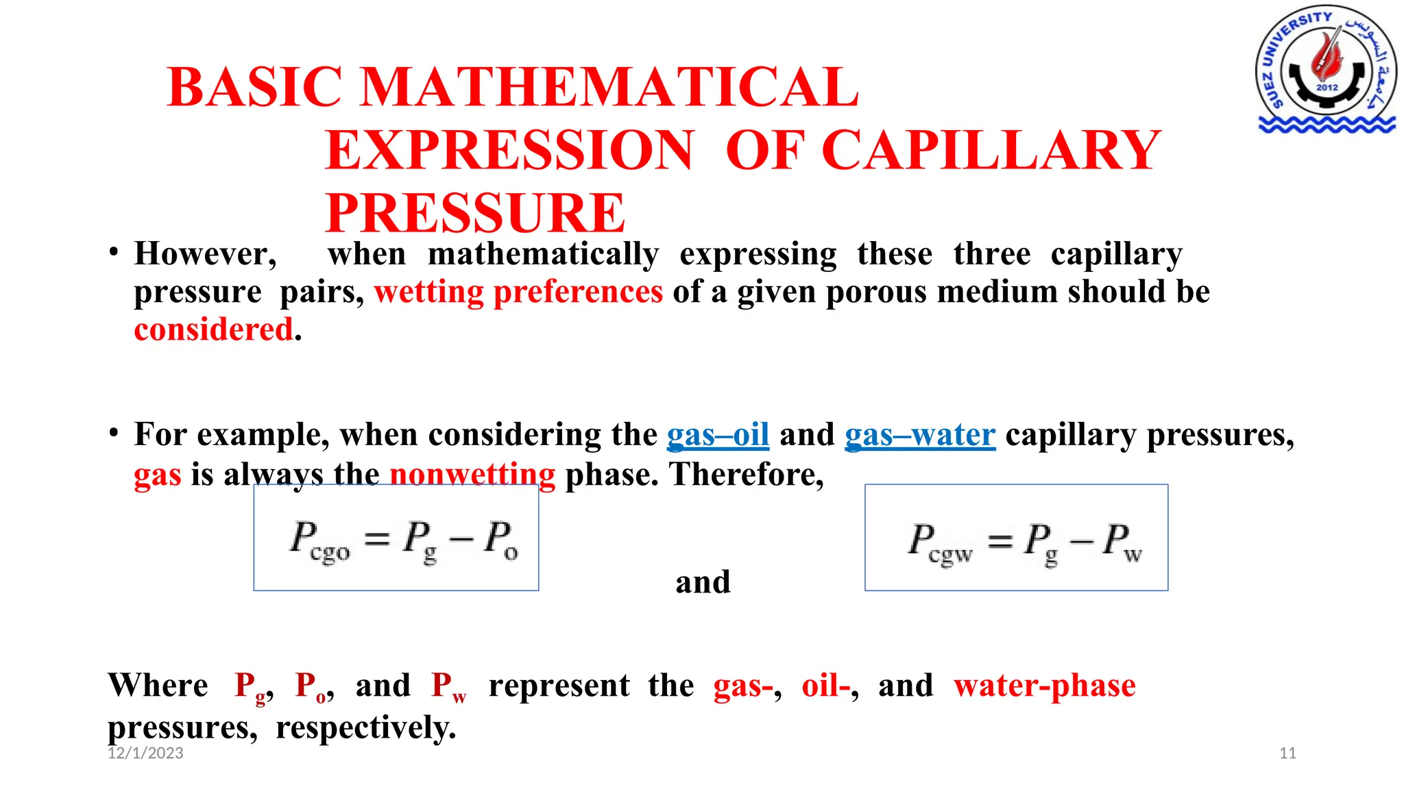
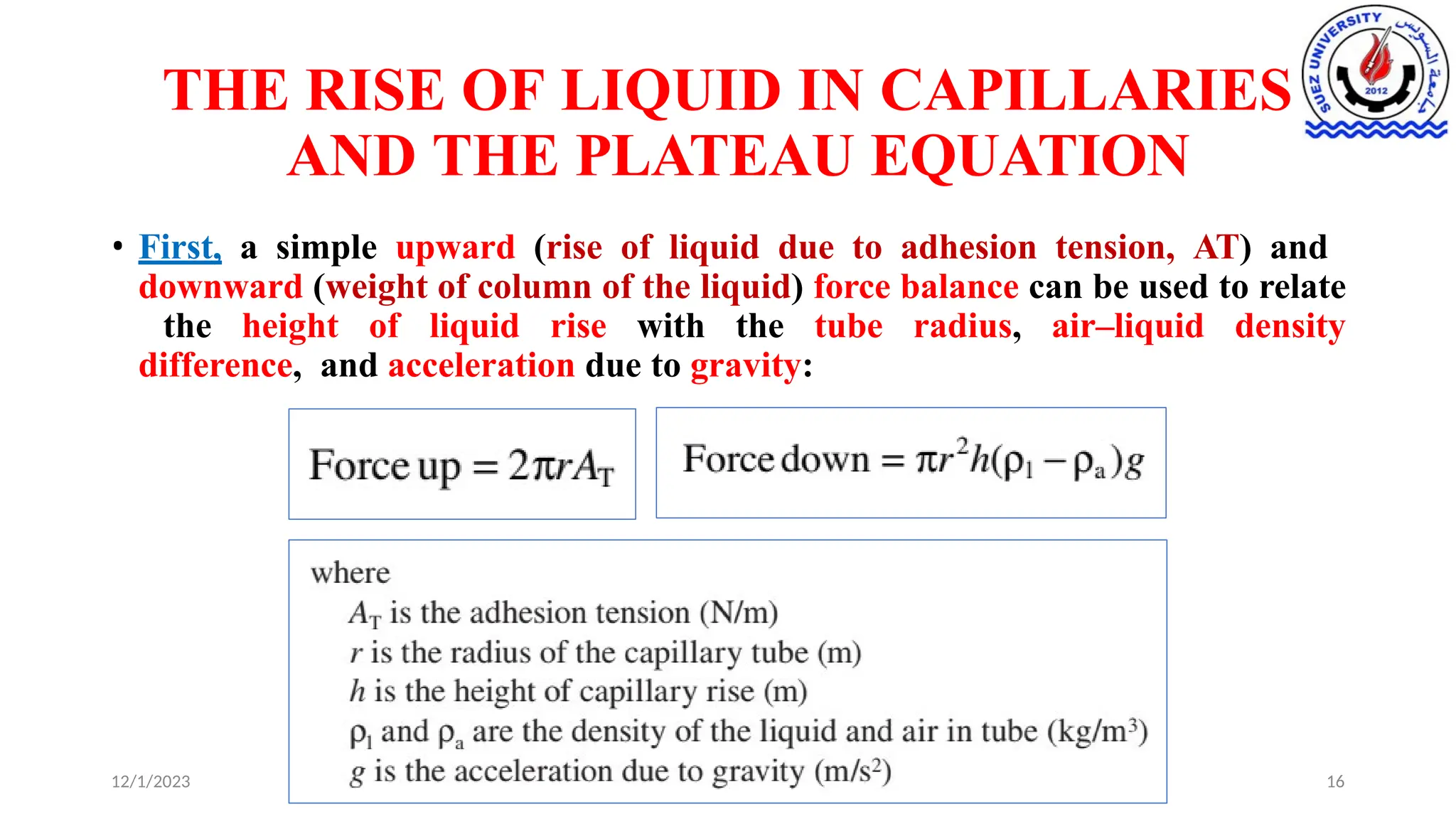
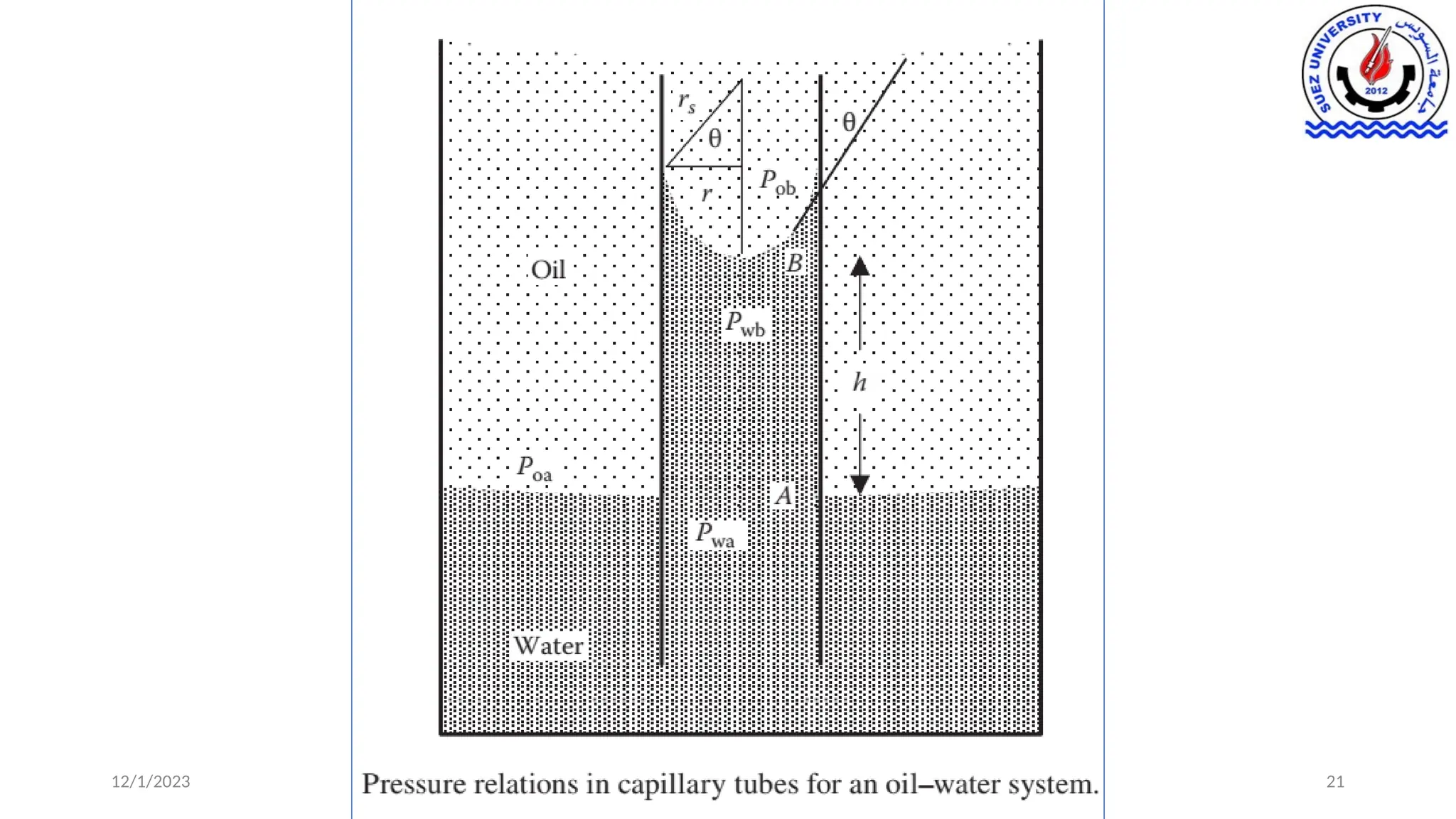
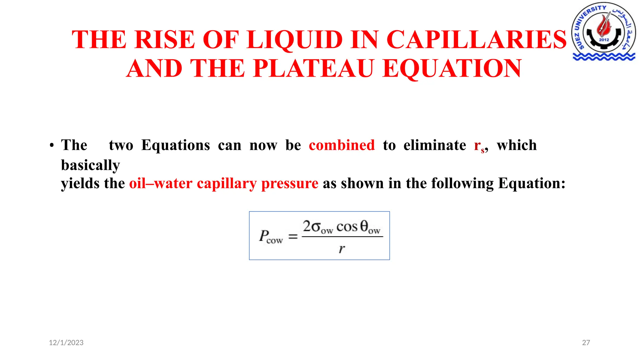
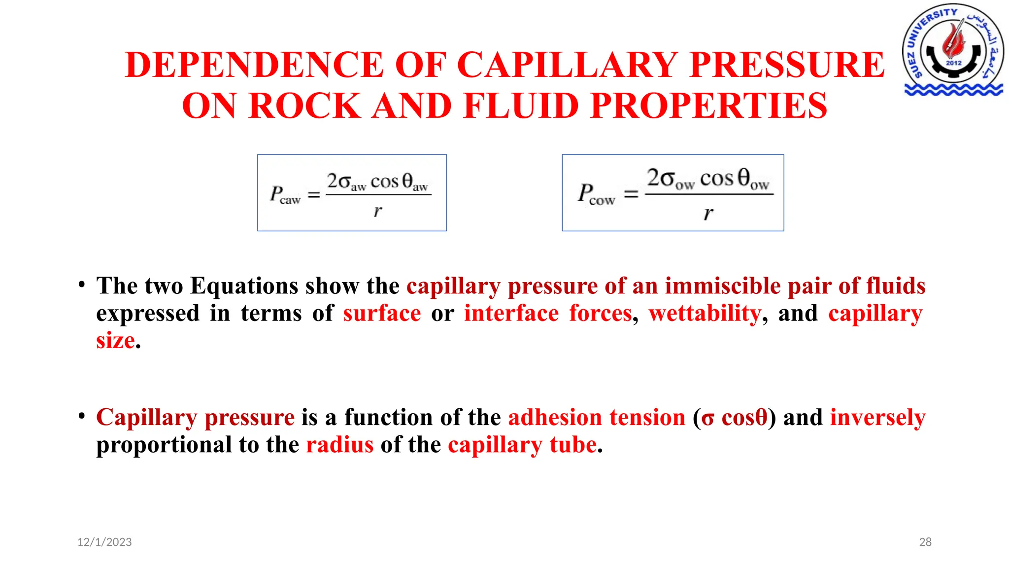
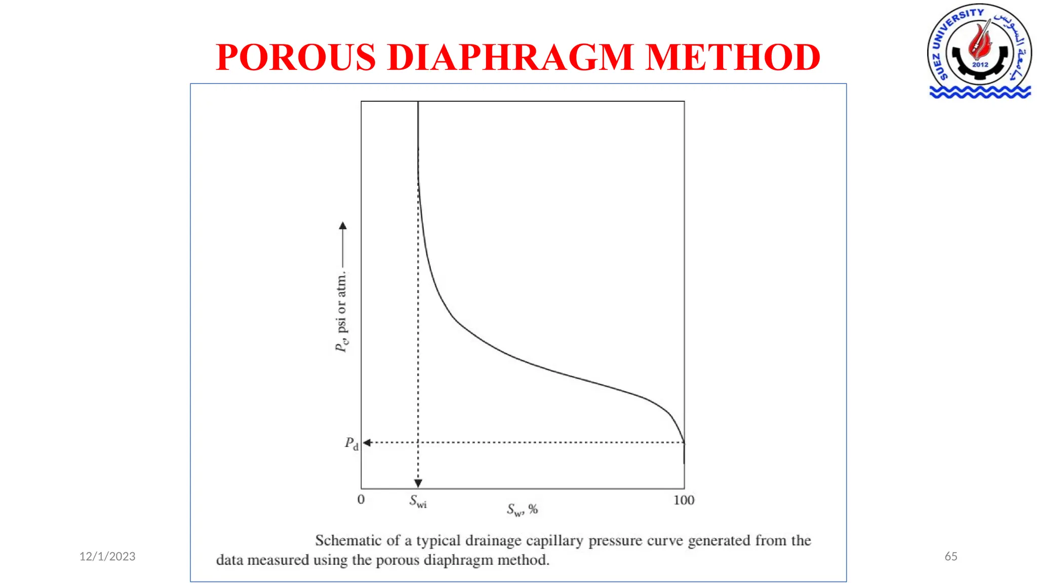
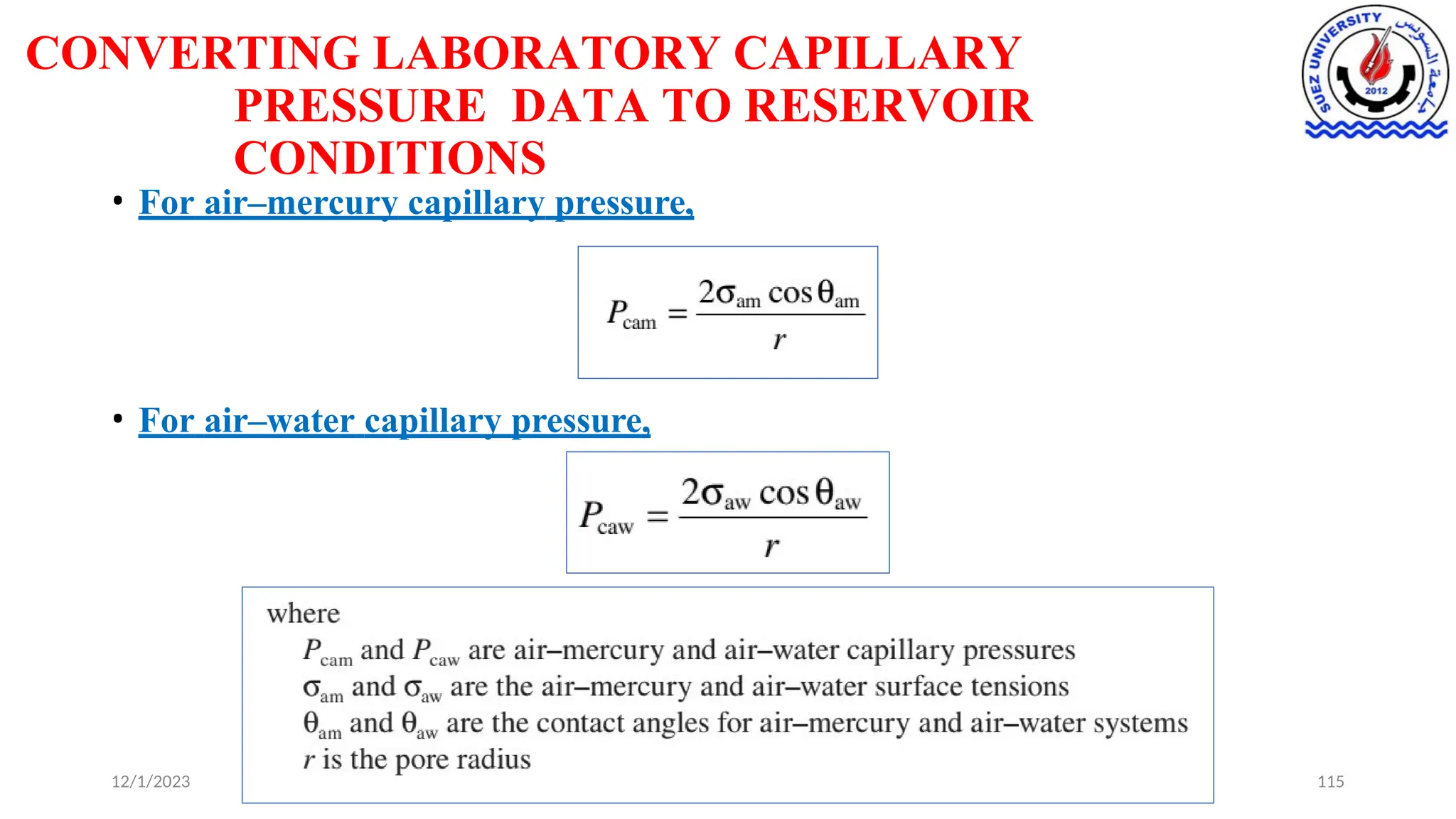
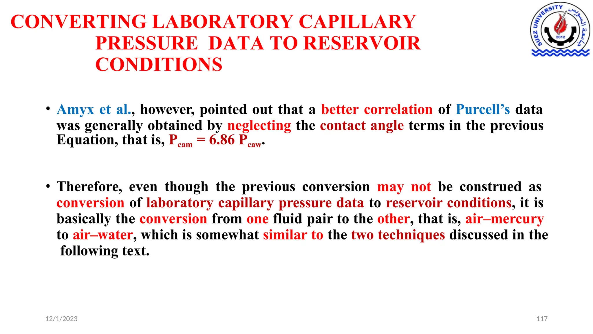
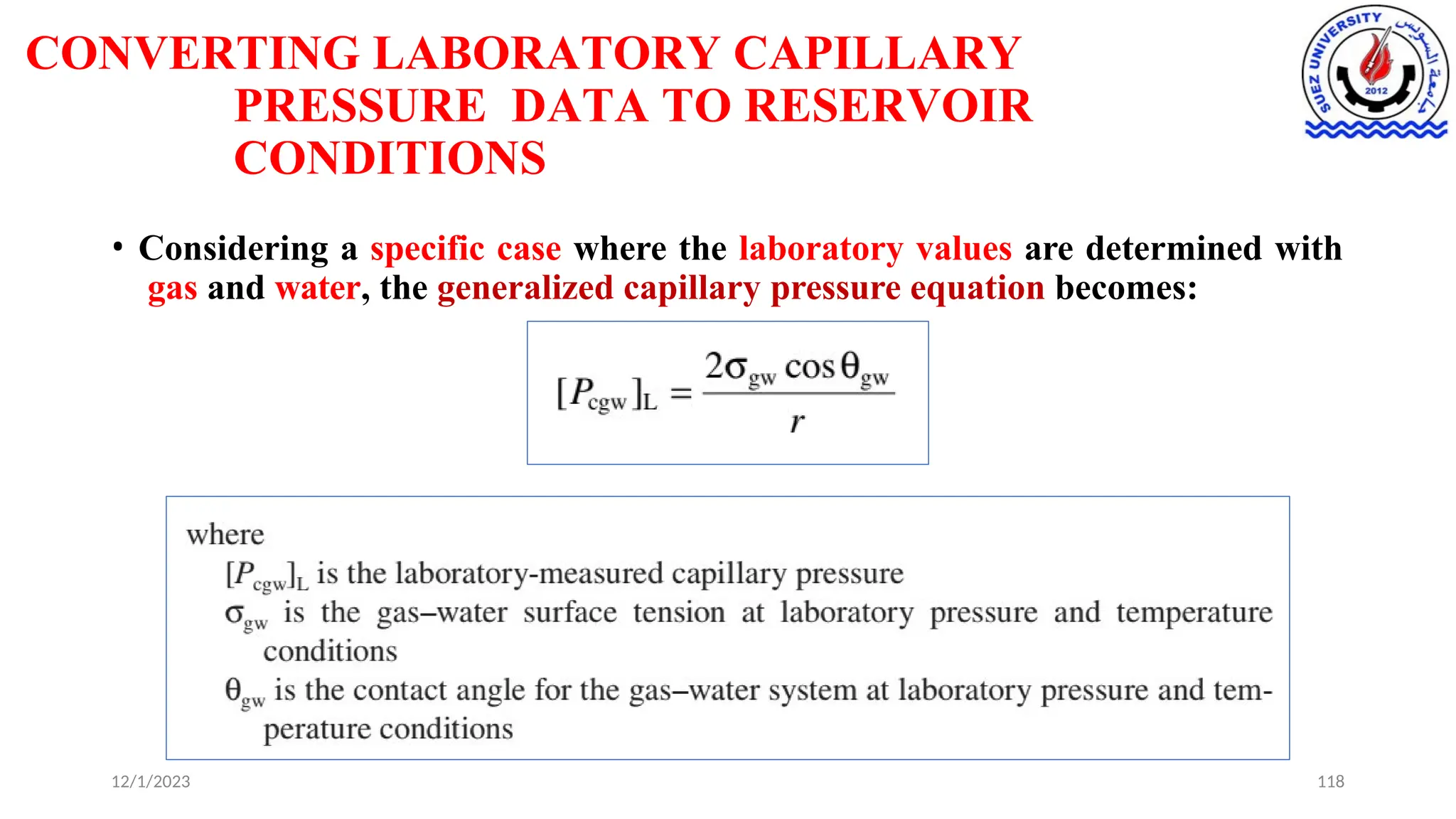
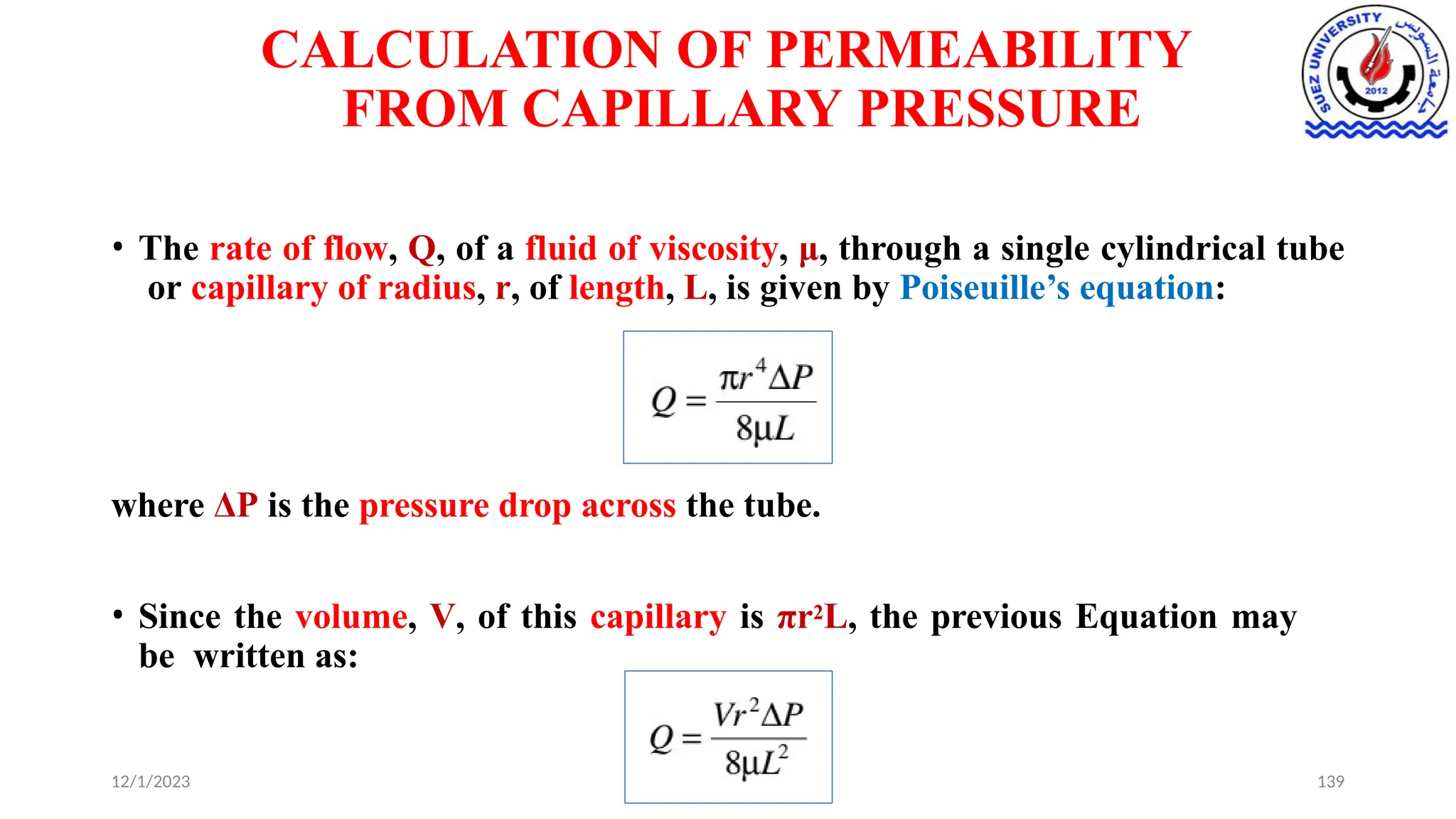
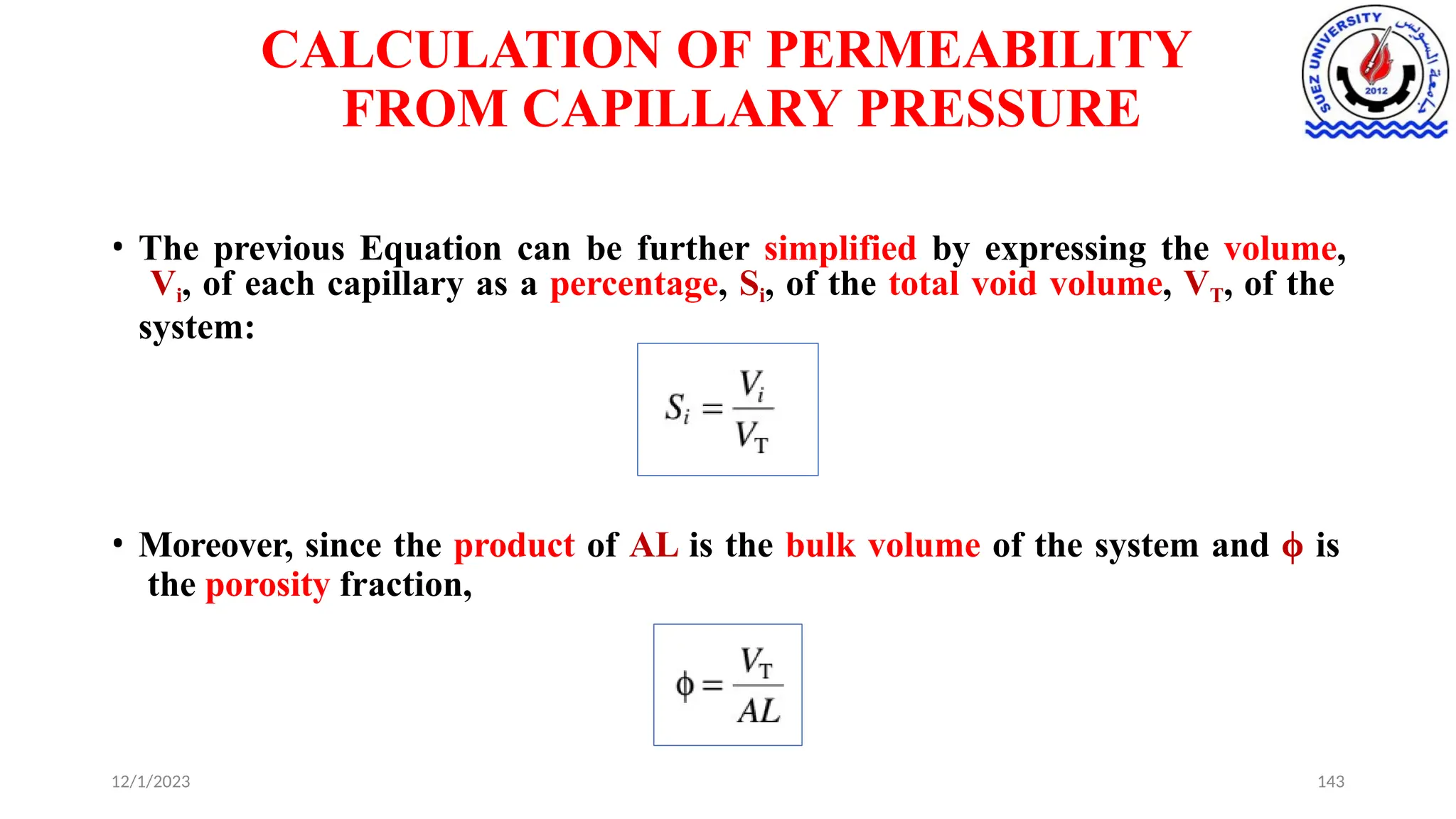
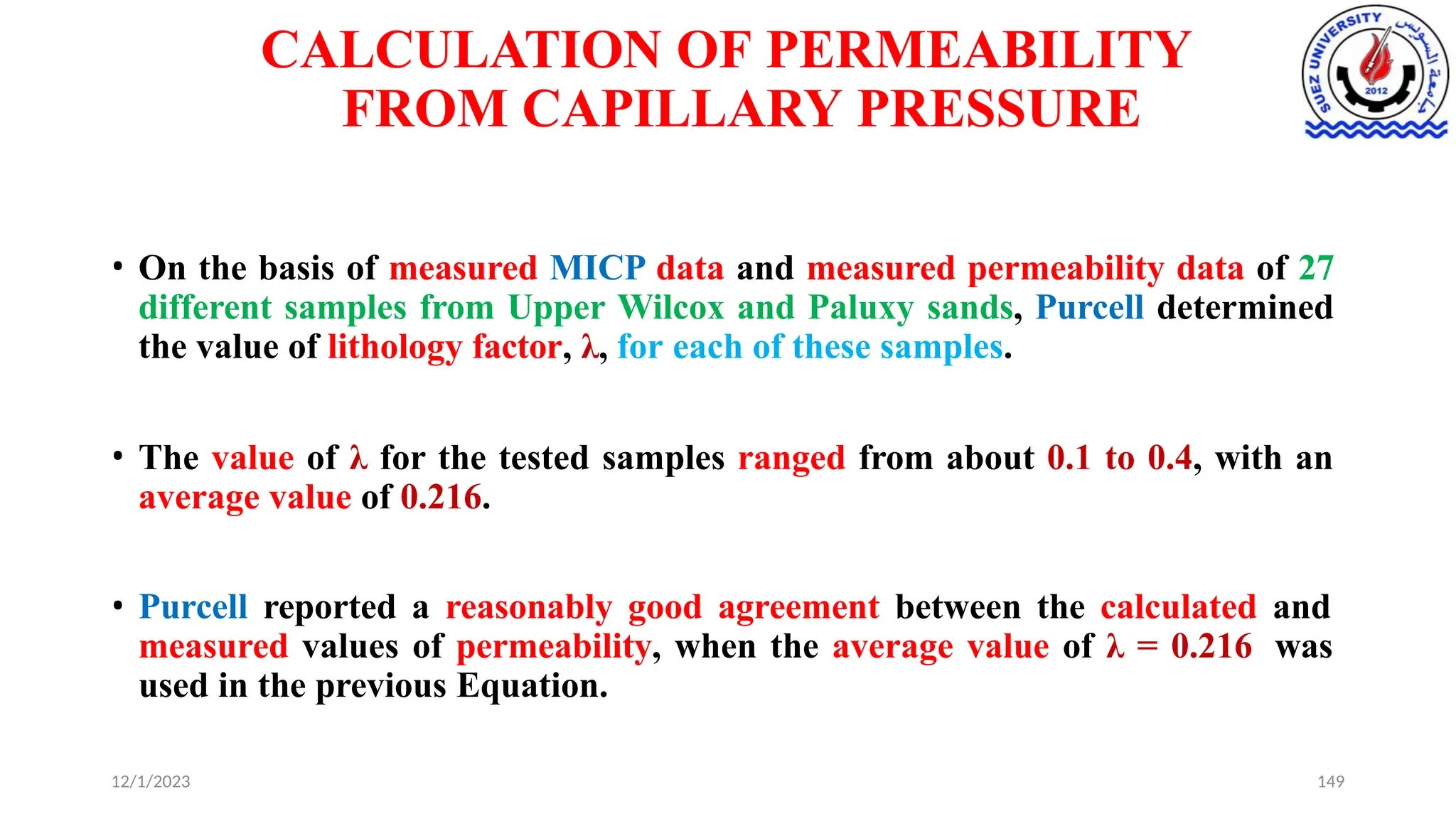
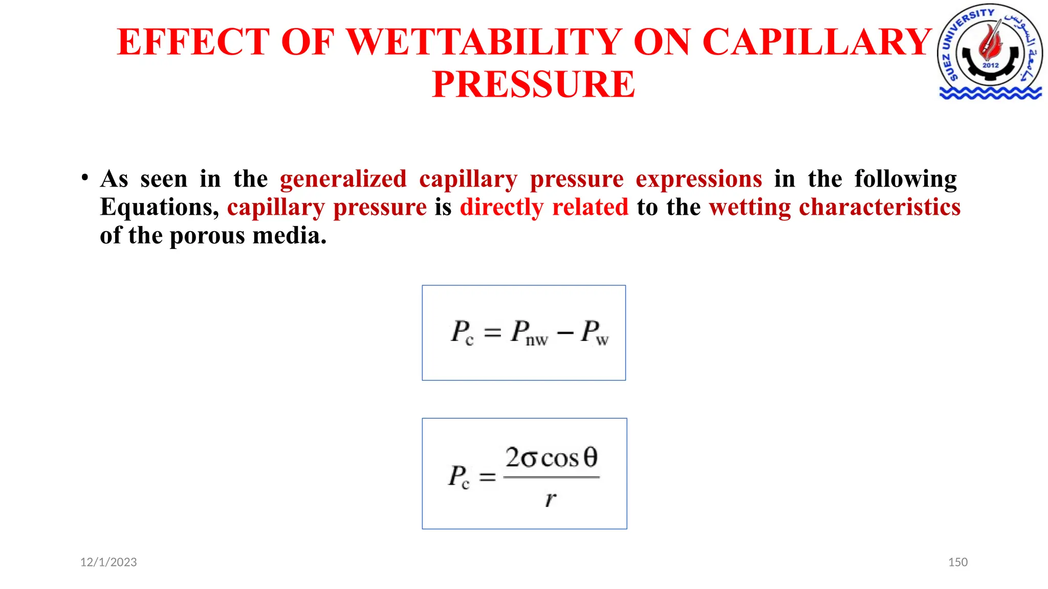
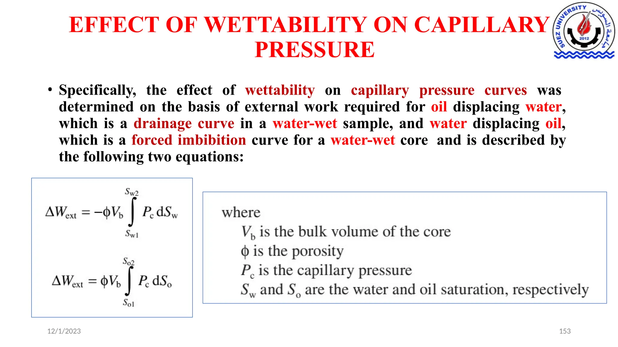
9. Capillary Pressure, its Measurements and Applications.pptx

CAPILLARY PRESSURE, ITS
MEASUREMENTS AND
APPLICATIONS
ALI MOUSTAFA ELSAYED WAHBA ELLAITHY
ASSISTANT PROFESSOR
PETROLEUM ENGINEERING DEPARTMENT
FACULTY OF PETROLEUM AND MINING ENGINEERING
SUEZ UNIVERSITY
E-mail: a.wahba@suezuni.edu.eg
Tel.: (+20) 1021122314 – (+20) 1555545827
1

INTRODUCTION
12/1/2023 2
• The previous chapter addressed the fact that the simultaneous existence of
two or more fluid phases in a pore space of a reservoir rock requires the
definition of surface and interfacial tensions (IFTs), wettability, capillary
pressure, and relative permeability.
• This chapter focuses on the capillary pressure characteristics of a porous
medium.

INTRODUCTION
12/1/2023 3
• Capillary pressure exists whenever reservoir rock pores,
which capillary sizes, are saturated with two or more immiscible fluid
phases.
are
of
• In 1941, Leverett first stated that the interfacial boundary between two
immiscible fluid phases present in a porous medium is curved due to IFT
between the fluids.
• He ascribed the sharpness of the curvature to the size of pores and the
properties of fluids.

INTRODUCTION
12/1/2023 4
• The interfacial curvature is the most significant property of the system from
the standpoint of capillary behavior, which gives rise to a difference in the
pressure across the interface, called capillary pressure, denoted by Pc.
• This basically means that each immiscible fluid has a pressure that is distinct
from that of the other immiscible fluids.
• As it will be mathematically shown later, capillary forces in petroleum
reservoirs are a manifestation of the combination of IFT, wetting
characteristics, and pore sizes of a given system.

INTRODUCTION
12/1/2023 5
• The presence of capillary forces in a porous medium causes hydrocarbon
entrapment.
• The classic example is the migration of hydrocarbons from a source rock to
the water-saturated reservoir rock; petroleum trapped in a reservoir
represents an equilibrium state between gravity that wants to move the
petroleum upward, which is resisted by capillary pressures.
• Leverett postulates that reservoir fluids owing to their long existence in
undisturbed mutual contact prior to exploitation are in substantial gravity–
capillary equilibrium.

INTRODUCTION
12/1/2023 6
• This is the primary reason why dense fluid such as water or brine (usually
represented by connate or irreducible water saturation) is found in petroleum
reservoirs at higher elevations above the oil–water contact (OWC).
• The equilibrium state thus manifests a particular fluid distribution, zonation,
and fluid contacts in a given petroleum reservoir, which is helpful in the
estimation of petroleum reserves and in other problems.

INTRODUCTION
12/1/2023 7
• Capillary forces also play a major role in the dynamic problems, involving
the flow of immiscible fluid phases in porous media under the influence of
capillarity, gravity, and an impressed external pressure differential.
• In reservoir flow processes before a bubble of gas or oil globule can flow
through a small pore diameter, the critical entry pressure or capillary
pressure must be overcome.
• For example, more than 1480 psi pressure would be theoretically required to
move a spherical oil globule through a 0.01 μm diameter pore, assuming an
oil–water IFT of 25 mN/m and complete wetting by water.

INTRODUCTION
12/1/2023 8
• Thus, it is clear from the foregoing that it is advantageous to understand the
nature of these capillary forces both from a static reservoir structure (in
terms of fluid contacts, transition zones, and free water level [FWL]) and the
dynamic actual hydrocarbon recovery standpoint.

BASIC MATHEMATICAL
EXPRESSION OF CAPILLARY
PRESSURE
• The interfacial boundary between the two immiscible phases is curved, which
is convex with respect to the nonwetting fluid, and the pressure within the
nonwetting fluid is greater than the pressure within the wetting fluid.
• Consequently, following Leverett’s definition and denoting the pressure in the
nonwetting phase and the wetting phase as Pnw and Pw, respectively, capillary
pressure is expressed as:
Capillary pressure = pressure in the nonwetting phase - pressure in the wetting
phase
12/1/2023 9

BASIC MATHEMATICAL
PRESSURE
12/1/2023 10
• The Equation is the defining equation for capillary pressure in a
porous medium. Basically, three types of capillary pressures exist:
1. Gas–oil capillary pressure denoted by Pcgo
2. Gas–water capillary pressure denoted by Pcgw
3. Oil–water capillary pressure denoted by Pcow

BASIC MATHEMATICAL
PRESSURE
• However, when mathematically expressing these three capillary
pressure pairs, wetting preferences of a given porous medium should be
considered.
• For example, when considering the gas–oil and gas–water capillary pressures,
gas is always the nonwetting phase. Therefore,
and
Where Pg, Po, and Pw represent the gas-, oil-, and water-phase
pressures, respectively.
12/1/2023 11

BASIC MATHEMATICAL
PRESSURE
• In the case of oil and water, either phase could preferentially wet the rock.
• Therefore, oil–water capillary pressure of a water-wet rock (water is
a wetting phase and oil is a nonwetting phase) can be expressed as
• Pcgo and Pcow can be combined if all the three phases are continuous, such that
12/1/2023 12

BASIC MATHEMATICAL
PRESSURE
12/1/2023 13
• However, given the fact that the capillary pressure is a combined effect of
IFTs, pore sizes, and wetting characteristics of a given system, a practical
mathematical expression that relates capillary pressure to these properties
should be developed.
• The development of such an equation, based on the rise of liquid in the
capillaries, and the Plateau equation is described in the following section.

THE RISE OF LIQUID IN CAPILLARIES
AND THE PLATEAU EQUATION
12/1/2023 14
• Amyx et al. have developed practical capillary pressure equations that relate
IFT, pore size, and wettability based on the rise of liquids in capillaries (see
the following Figure).

• First, a simple upward (rise of liquid due to adhesion tension, AT) and
downward (weight of column of the liquid) force balance can be used to relate
the height of liquid rise with the tube radius, air–liquid density
difference, and acceleration due to gravity:
12/1/2023 16

• However, based on the definition of adhesion tension, AT =
σal*cosθal; therefore,
12/1/2023 17

• Second, as per the definition of capillary pressure, a difference in pressure
exists across the air–liquid interface, which can be expressed as:
• A combination of the two Equations leads to the capillary pressure equation
in terms of surface forces, wettability, and capillary size:
12/1/2023 18

• If the liquid in the tube shown in the Figure is water, then:
• If the air–water surface tension and the capillary radius are expressed in N/m
and m, respectively, then the capillary pressure is in N/m2.
12/1/2023 19

• An expression similar to the previous Equation can also be developed for two
immiscible liquids, such as the capillary tube immersed in a beaker of water
where oil is the other liquid, as shown in the Figure.
• For such a system, the subscripts a and l in the previous Equation can be
replaced by o for oil and w for water, and thus oil–water capillary pressure
expressed as:
12/1/2023 20

• Tiab and Donaldson have stated that the microscopic observations of
immiscible fluids using glass beads and sand grains have established the
complex geometrical aspects of the liquid–liquid and liquid–solid contacts
and the curved interfacial boundary.
• A general expression for capillary pressure as a function of IFT and
curvature of the interface is due to Plateau:
12/1/2023 22

12/1/2023 23
• In the earlier equation, R1 and R2 are the principal radii of curvature of the
interface, and σ is IFT.
• Practically speaking, the principal radii of curvature are impossible to
measure as they are determined by the local pore geometry, wettability,
saturation, and the saturation history.

• Anderson used a simple capillary tube system such as the one in the following
Figure to obtain equivalent expression for the radii of curvature to arrive at
the capillary pressure equation shown in the following Equation.
12/1/2023 24

• When the capillary tube in consideration is small enough, the interface can be
approximated as a portion of a sphere, which has a radius rs, and since the
surface is spherical, both radii of curvature are equal to rs such that
• Based on the geometry, the cosine of contact angle θ is
Where r is the capillary tube radius.
12/1/2023 26

• The two Equations can now be combined to eliminate rs, which
basically
yields the oil–water capillary pressure as shown in the following Equation:
12/1/2023 27

DEPENDENCE OF CAPILLARY PRESSURE
ON ROCK AND FLUID PROPERTIES
• The two Equations show the capillary pressure of an immiscible pair of fluids
expressed in terms of surface or interface forces, wettability, and capillary
size.
• Capillary pressure is a function of the adhesion tension (σ cosθ) and inversely
proportional to the radius of the capillary tube.
12/1/2023 28

DEPENDENCE OF CAPILLARY
PRESSURE ON ROCK AND FLUID
PROPERTIES
12/1/2023 29
• Now we make a qualitative examination of the effect of pore size (capillary
radius in this case) and the adhesion tension on capillary pressure.
• The following Figure shows the effect of varying the wetting characteristics of
the system and varying the radius of the capillary tube.

PROPERTIES
12/1/2023 30

PROPERTIES
12/1/2023 31
• In Figure case (a), the wetting characteristics are the same, that is, the same
IFT and contact angle, but the radius of the capillary tube is different.
 In this case, the capillary pressure is inversely proportional to the
capillary tube radius, while the adhesion tension remains constant.
 By merely looking at the mathematical expression of capillary pressure, it
is easily understood that the higher the capillary tube radius, the lower
the capillary pressure, or vice versa.
 Alternatively, in terms of the weight of the liquid column, in the case of
higher capillary tube radius, obviously the gravity forces are dominating
because the weight of the liquid column increases and consequently the
capillary pressure decreases.
 The opposite is true in the case of the smaller capillary tube radius.

PROPERTIES
12/1/2023 32
• On the other hand, when the capillary tubes of same radius but different
wetting characteristics are considered, the denominator in the capillary
pressure equation will be a constant, and the value of capillary pressure will
be directly proportional to the adhesion tension or the wetting characteristics
of the system.
• The Figure case (b) shows such a system of same radius and different contact
angles.
• In this case, the smaller the contact angle, the greater the height of liquid rise
and stronger the adhesion tension, leading to higher capillary pressure,
whereas the opposite is evident from the other tube having weaker wetting
characteristics or adhesion tension that obviously results in lower capillary
pressure.

CAPILLARY PRESSURE AND
SATURATION HISTORY
12/1/2023 33
• The previous section looked at a static case of capillary pressures, purely
from a mathematical standpoint, only considering the effects of varying
adhesion tension and pore size (single capillary tube radius).
• However, saturation of the two immiscible phases and the history was
not
considered in the discussion (essentially a point value of Pc).

SATURATION HISTORY
12/1/2023 34
• Additionally, the phenomenon described earlier for a single capillary tube
also exists when bundles of interconnected capillaries of varying sizes exist in
a porous medium.
• The capillary pressure that exists within a porous medium between two
immiscible fluid phases is a function of adhesion tension and the average size
of the capillaries.

SATURATION HISTORY
12/1/2023 35
• Additionally, as mentioned earlier, capillary pressure is also a function of the
saturation distribution of the fluids involved and the saturation history.
• As the relative saturations of the phases change, the pressure differences
across the fluid interfaces also change, resulting in a change in the capillary
pressure.
• This is obviously of great significance when considering both static and
dynamic problems of hydrocarbon reservoirs.

SATURATION HISTORY
12/1/2023 36
• Static problems primarily involve fluid distribution, fluid contacts, and
zonation in the reservoirs; dynamic problems consist of the transport of
immiscible fluid phases in the pore spaces under the influence of forces due to
gravity, capillarity, and an impressed external pressure gradient.
• Therefore, it is imperative to study the effect of saturation distribution and
saturation history on capillary pressure.
• However, before saturation distribution and saturation history can be
discussed, we define two important saturation processes, namely, imbibition
and drainage, that are dependent on the wetting characteristics of fluid
phases.

CAPILLARY PRESSURE AND SATURATION
HISTORY
12/1/2023 37
• When oil and water are the two fluid phases in a porous medium, generally
either oil or water will preferentially wet the pore space based on which the
phases will be identified as wetting or nonwetting.
• Thus, in a porous medium saturated with oil and water, two basic processes
can occur—a wetting phase displacing a nonwetting phase and a nonwetting
phase displacing a wetting phase.
• These two processes are called imbibition and drainage, respectively. For
instance, when water displaces oil from a water-wet rock, the process is
imbibition, and when water displaces oil from an oil-wet rock, the process is
drainage.
• However, when gas displaces oil or water, the process is always drainage
because gas is always the nonwetting phase in comparison to oil or water.

SATURATION HISTORY
12/1/2023 38
• To understand the dependence of capillary pressure on fluid saturation
distribution and saturation history (resulting from imbibition or drainage), a
continuous capillary tube that changes in diameter from small to large to
small or a void space geometry with many bottlenecks is considered as a
hypothetical porous medium.
• The following Figure: cases (a) and (b) represent the drainage sequence, and
cases (c) and (d) represent the imbibition sequence, respectively.

SATURATION HISTORY
12/1/2023 39

SATURATION HISTORY
12/1/2023 40
• In the drainage sequence, initially wetting-phase saturation is 100%, but
when it is reduced to 90%, the corresponding Pc (X psi) across the interface,
which is equal to the applied pressure and the pressure due to the column of
the suspended liquid, is high.
• In other words, the system is 90% saturated with the wetting phase for a
higher value of Pc.

SATURATION HISTORY
12/1/2023 41
• In the imbibition sequence, initially the wetting-phase saturation is 0%, but
the tube is immersed in a container filled with the liquid that will
preferentially wet the tube.
• Naturally, the wetting liquid will begin to imbibe, as we saw in the case of
simple capillary tube geometries, until the adhesion force is balanced by the
weight of the liquid column, resulting in a wetting-phase saturation of 20%.
• However, the value of Pc corresponding to this wetting-phase saturation is
also X psi.

SATURATION HISTORY
12/1/2023 42
• In summary, in the earlier oversimplified drainage and imbibition sequence,
wetting-phase saturations of 90% and 20% are obtained for the identical
value of Pc.
• Nevertheless, the dependence of the capillary pressure–saturation (wetting
phase) relationship on the saturation process or history can be realized; that
is, for a given capillary pressure, a higher value of wetting-phase saturation is
obtained in the drainage process than when imbibition takes place.
• Bear states that as long as the porous medium remains stable, the saturation
history loop and corresponding capillary pressures can be repeatedly
retraced.

SATURATION HISTORY
12/1/2023 43
• Thus, this Section and the previous one basically establish the dependence of
capillary pressure–saturation relationship on the size (r) and distribution of
the pores, fluid characteristics (σ) and their wetting preferences with the
given rocks (θ), and the history of the saturation process, which is an
important consideration before the data are actually applied to reservoir
engineering calculations.

LABORATORY MEASUREMENT OF
CAPILLARY PRESSURE
12/1/2023 44
• Following the two primary displacement processes in the porous medium,
laboratory measurement of capillary pressure is confined to imbibition and
drainage.
• In all the laboratory measurement methods, wetting-phase saturation is
increased in the imbibition process, while in the drainage process, wetting-
phase saturation is decreased from a maximum value (typically 100%) to the
irreducible minimum by increasing the capillary pressure from 0 to a large
positive value.
• The plots of capillary pressure data obtained in such a fashion are called
imbibition and drainage capillary pressure curves, respectively.

CAPILLARY PRESSURE
12/1/2023 45
• All laboratory experiments are basically designed to first mimic or simulate
the saturation history of the reservoir, that is, migration of hydrocarbons
from source rocks into water-filled reservoir rocks.
• Under the assumption that the rocks are water wet, at least prior to
hydrocarbon migration, this is accomplished by the drainage process by
displacing the wetting phase (water) by a nonwetting phase (oil or gas), which
primarily establishes the fluid saturations that are found when the reservoir
is discovered.

CAPILLARY PRESSURE
12/1/2023 46
• On the other hand, oil production performance (oil as a nonwetting phase) is
generally governed by the imbibition process.
• Therefore, imbibition capillary pressure curves are generally used
in reservoir studies.

CAPILLARY PRESSURE
12/1/2023 47
• In almost all laboratory measurement methods, capillary pressures are
measured on cylindrical core plug samples of the representative formation.
• The laboratory measured imbibition and drainage capillary pressure–
saturation relationships can be construed as somewhat equivalent to
measuring these relationships for a bundle of several capillaries of varying
tortuosities and sizes.
• Generally, two types of core samples can be used to carry out capillary
pressure measurements: preserved state or native state or cleaned and dried
samples.

CAPILLARY PRESSURE
12/1/2023 48
• For cleaned and dried samples, the drainage cycle can begin with 100%
wetting-phase saturation down to the irreducible wetting-phase saturation.
• Before the core samples are used in capillary pressure measurements,
appropriate cleaning and drying protocols must be followed so as not to alter
the natural fabric of the rock considering the strong proportionality of
capillary pressure to adhesion tension or wettability.
• Therefore, the use of appropriate core material in capillary pressure
measurements is always an issue.

CAPILLARY PRESSURE
12/1/2023 49
• If preserved- or native-state core samples are to be used for capillary pressure
measurements to maintain the original wettability, such samples would then
be presumed to already have an irreducible or initial water saturation.
• Then, the core sample is normally flooded with representative formation
water or brine so that a maximum in the wetting-phase saturation is obtained
(under the presumption that the sample is water wet).

CAPILLARY PRESSURE
12/1/2023 50
• This saturation is then reduced in steps by injecting a nonwetting phase to
mimic the original reservoir fluid distribution.
• Subsequently, the imbibition cycle can be completed by increasing the
wetting-phase saturation.
• Some of the most commonly used laboratory techniques for measuring
capillary pressures are covered in the following sections, beginning with the
pioneering experiments of Leverett on capillary pressures of sandpacks.

LEVERETT’S CAPILLARY PRESSURE
EXPERIMENTS
12/1/2023 51
• The pioneering work of Leverett in 1941 introduced the concept of capillary
pressure measurement to the petroleum industry.
• Leverett conducted capillary pressure–saturation experiments on
six different unconsolidated sandpacks.
• The sands used in his experiments were of different mesh sizes and packed in
vertical glass and brass tubes.
• Out of the six sands that he used; two sands contained claylike material.

EXPERIMENTS
12/1/2023 52
• Leverett designed and conducted the experiments in such a manner that both
imbibition and drainage capillary pressure curves were obtained.
• The drainage curves were obtained by desaturating (from 100% water- or
wetting-phase saturation) the water-saturated sandpack with one of its end
lowered into a container having FWL.
• The imbibition curves were obtained by lowering the tubes packed with dry
sand (100% air or nonwetting-phase saturation) into the water container so
that water was imbibed by the sandpack due to capillary forces.
• The water saturation in the tube was determined at various positions above
the FWL in the container for both imbibition and drainage.

EXPERIMENTS
• As shown in the following Figure schematically, Leverett plotted the results of
his experiments in a dimensionless form, expressed by the following
Equation, versus water saturation.
• Leverett proposed the dimensionless correlating function to generalize the
capillary pressure data for different sands:
53
12/1/202
3
The variables in the Equation
can be expressed in any
consistent set of units to yield
a dimensionless function.

EXPERIMENTS
12/1/2023 55
• Leverett observed that although the data for four of the sands fell
satisfactorily near the two curves, one for imbibition and the other for
drainage, differences between the two groups were obvious.
• This difference in the imbibition and drainage curves is due to an effect
known as hysteresis, which is dependent on the saturation history, similar to
what was seen in the case of the simplified example discussed in the previous
Section.
• The hysteresis effect in capillary pressure curves is discussed in the next
Section in greater detail.

EXPERIMENTS
12/1/2023 56
• Out of the six sands studied by Leverett, two of the sands containing clay-
laden material, however, did not correlate as per the data presented for the
four sands, but the general trend was similar.
• The results in fact indicated that more water was retained by the clay-laden
sands at large values of h, the height, and less at small ones, in comparison to
the four clean sands.
• Leverett ascribed this observation to the fact that clays absorb water, that is,
the water so taken up being held more tightly than the same amount of water
that would be held by capillarity.

EXPERIMENTS
12/1/2023 57
• Although Leverett’s experiments constituted the most fundamental and
original work attempted toward measuring or establishing the capillary
pressure–saturation relationships, it is not feasible to determine the capillary
properties of reservoir rock core materials by a method such as Leverett’s.
• Therefore, other practical methods of measuring the capillary pressure have
been devised and are routinely used in the petroleum industry as part of
SCAL.
• These methods are discussed in the following three sections.

POROUS DIAPHRAGM METHOD
12/1/2023 58
• The porous diaphragm method, proposed by Welge and Bruce in 1947, is
schematically illustrated in the following Figure.
• This is perhaps one of the simplest methods to determine the capillary
pressure–saturation relationships for core plug samples.
• The method is based on the drainage of a core sample initially saturated with
a wetting fluid, which is placed inside a chamber filled with a
nonwetting fluid.

12/1/2023 59

12/1/2023 60
• The wetting-phase-saturated core rests on a layer of the contact material
(Kleenex) and a porous diaphragm or membrane made up of fritted glass or
porcelain, initially saturated with the fluid to be displaced.
• The basic requirement is that the membrane will have uniform pore size
distribution (PSD) containing pores of such size that the selected displacing
fluid will not penetrate the membrane when the pressure applied to the
displacing fluid is below some predetermined value (threshold pressure).

12/1/2023 61
• As shown in the Figure, the core sample is 100% saturated with reconstituted
formation water or brine.
• The test sample is subjected to displacement of water by crude oil in a
stepwise fashion.
• The pressure is applied to the crude oil via nitrogen.
• The pressure applied is essentially the capillary pressure, Po–Pw. On achieving
static equilibrium, capillary pressure and the corresponding wetting-phase
saturation in the core based on the displacement in the scaled graduated tube
is recorded. This basically constitutes one Pc–Sw data point on the curve.

12/1/2023 62
• The test is terminated at a certain value of maximum pressure at which no
more water is produced, also an indication that irreducible water saturation
is reached.
• Any combinations of fluid pairs can be used such as gas–oil, oil–water,
or
gas–water.
• In principle, the setup can also be modified suitably to obtain imbibition
curves.

12/1/2023 63
• Another variant of the diaphragm method is the technique proposed by Cole
developed primarily to determine the magnitude of the connate water
saturation.
• In principle, the technique is similar to the original diaphragm method.
• The core initially 100% saturated with the formation water is subjected to
increasing air pressure which displaces the water from the core, and the test
continues until no more water is produced.

12/1/2023 64
• The drainage capillary pressure versus wetting-phase saturation curve
generated by the porous diaphragm method is schematically shown in the
following Figure and its important features discussed in the next Section.

12/1/2023 65

MERCURY INJECTION METHOD
12/1/2023 66
• The mercury injection technique is one of the most commonly used methods
in the petroleum industry for rapid measurement of the capillary pressure of
reservoir rock samples.
• The method was originally proposed by Purcell in 1949.
• In this technique, the two phases in consideration are air and mercury,
respectively; the former is the wetting phase, while the latter is the
nonwetting phase.
• Given the known nonwetting characteristics of mercury with respect to
reservoir rocks, its use is generally preferred because there is no ambiguity as
far as the oil- or water-wetting tendencies are concerned, if they are the two
phases to be used in a capillary pressure test.

12/1/2023 67
• The schematic and the actual picture of the mercury injection capillary
pressure (MICP) setup are shown in the following Figure.
• The essential components of the setup include a mercury hand pump with a
vernier scale for taking volume readings, a pycnometer that houses the core
sample and mercury, nitrogen cylinder for pressurizing the mercury, and a
display for reading pressure values.

12/1/2023 69
 The basic procedure for conducting the measurements is
as follows:
• Prior to forcing mercury into the core, the initial step involves the
determination of a volume correction factor due to mercury compressibility.
• This is done by placing a solid stainless steel core (roughly the same size as
the actual core) into the pycnometer and subsequently pressurizing the
mercury surrounding the solid core and noting the corresponding changes in
the mercury levels in the pycnometer reference windows.

12/1/2023 70
• This change in the volume is then compensated by the hand pump, and the
difference gives the volume change (read through the vernier scale) due to
mercury compressibility effect.
• An entire correlation is then established for the range of pressures to be
tested. Subsequently, a clean and dry (thus 100% air saturated; air is the
wetting phase) core sample, of known porosity, to be tested is placed in the
pycnometer and its BV is determined.
• This is done at atmospheric pressure using the mercury levels in
the
pycnometer reference windows and the compensation by the hand pump.

12/1/2023 71
• Following this, the injection of mercury can begin.
• First, a certain low pressure (Pc) is applied to the mercury in the pycnometer
via a nitrogen cylinder.
• The volume of mercury forced into the pore spaces is then determined using
the same principle of mercury levels changing in the pycnometer, which are
adjusted by the hand pump.

12/1/2023 72
• The volume correction due to mercury compressibility corresponding to the
applied pressure is then subtracted from the volume of mercury in the core
measured previously, and the resulting value is termed Vinj, which is divided
by the sample pore volume to give the mercury saturation in the core.
• The injection procedure is typically continued until no more mercury can be
invaded into the pore spaces.
• The pressures and saturations measured in the earlier fashion determine the
drainage capillary pressure–saturation curve (mercury displacing air).

12/1/2023 73
• After reaching the maximum value of mercury saturation in the sample, a
mercury withdrawal capillary pressure curve can be determined by
decreasing the pressure in increments and recording the volume of mercury
withdrawn.
• The process continues until a limit is approached where the mercury ceases to
be withdrawn.
• The capillary pressure–saturation relationship determined in this manner
basically constitutes the imbibition capillary pressure–saturation curve (air
displacing mercury).

12/1/2023 74
• As an example, a typical drainage and imbibition MICP data are shown in
the following Figure.
• As an added benefit, the measured capillary pressure data can also be used to
determine PSD.
• Some of the disadvantages are as follows:
The core sample is rendered useless for any other further studies.
The toxicity of mercury, which constitutes a potential health hazard.

12/1/2023 75

CENTRIFUGE METHOD
12/1/2023 76
• A third commonly used method for determining the capillary pressure
properties of reservoir rocks is the centrifuge method.
• Apparently, the first capillary pressure experiments with a centrifuge
published in the petroleum literature were those of McCullough et al.,
followed by Hassler et al. in 1944.
• However, the centrifuge procedure that is used today was introduced by
Slobod et al.
• The procedure described here is that of Slobod et al.

CENTRIFUGE METHOD
12/1/2023 77
• The determination of the capillary pressure curve, for example, for an air–
water system, begins with complete water saturation of a cleaned and dried
core sample that is placed in a centrifuge tube according to an arrangement
such as the one shown in the following Figure.

CENTRIFUGE METHOD
12/1/2023 78

CENTRIFUGE METHOD
12/1/2023 79
• The system is rotated at a number of different speeds (so that the nonwetting
phase, air, displaces water, the wetting phase) selected to cover pressure
differences between phases required for the particular core.
• At each speed, the rate of rotation is maintained constant until no additional
water is displaced by air.

CENTRIFUGE METHOD
• The speed of rotation is converted into capillary pressure at the inlet end of
the core according to the following equation:
12/1/2023 80

CENTRIFUGE METHOD
12/1/2023 81
• The average water saturation in the core sample is determined by subtracting
the volume of displaced water from the original water content.
• However, the capillary pressure calculated using the previous Equation is the
capillary pressure at the inlet end of the core, whereas the saturation
measured from the amount of fluid displaced is the average saturation.
• Therefore, to use centrifuge-derived capillary pressure data, it must be
related to the saturation at the inlet end.

CENTRIFUGE METHOD
12/1/2023 82
• Tiab and Donaldson have discussed the procedures for calculating the
saturations at the inlet end using the approximate and theoretically exact
methods.
• The data obtained in this manner constitute the drainage capillary pressure
curve, because air is always the nonwetting phase when air–water or air–oil
pairs are considered.
• By following a somewhat similar procedure after incorporating alterations in
the setup, imbibition capillary pressure curves can also be obtained by using
the appropriate fluid pairs.
• Again, somewhat similar to the mercury injection method, the centrifuge
technique is cited for increased speed of obtaining the capillary pressure data.

CHARACTERISTICS OF CAPILLARY
PRESSURE CURVES
12/1/2023 83
• We will now focus on the salient features or characteristics of typical
capillary pressure–saturation curves.
• First consider the capillary pressure data presented in the following Figure,
measured by the diaphragm method for the air–water system.
• The Figure easily identifies the capillary pressure curve bound within two
saturation end points, and corresponding to these two end points, there are
capillary pressure end points.

PRESSURE CURVES
12/1/2023 84
• These two end points are some of the most notable features or characteristics
of the capillary pressure curves.
• In order to understand capillary pressure–saturation relationships, the scales
of saturation and capillary pressure are examined individually in the
following sections.

PRESSURE CURVES
12/1/2023 86
• An important aspect of capillary pressure curves is the noticeable difference
between the imbibition and the drainage capillary pressure curves seen in the
Figure, based on Leverett’s work on sandpacks, and the Figure, for a North
Sea core plug sample.
• This particular difference in the imbibition and drainage capillary pressure
curves is due to the phenomenon of capillary hysteresis, which is discussed in
the next Sections.

PRESSURE CURVES
12/1/2023 87
• Another important characteristic of the capillary pressure curves to be
considered is their relationship with permeability.
• Even though a given rock permeability does not impart any specific or
particular characteristic to the capillary pressure curves, it certainly
influences the location of the capillary pressure–saturation curves when these
data are plotted on a single graph for rock samples of different permeabilities
(see the next Sections).

SATURATION SCALE
12/1/2023 90
• The saturation scale in the third Figure includes the mercury saturation, SHg,
or the air saturation, which is (1 – SHg), beginning with 0% mercury
saturation, or 100% air saturation, which can also be construed as 100%
water saturation.
• This is because, in this case, the wetting phase (air) is being displaced by the
nonwetting phase (mercury); that is, the drainage curve can also be carried
out with an air–water pair, and the process is designed to mimic the upward
migration of hydrocarbons in a reservoir rock.
• Tracing the saturation–capillary pressure path backward on the curve that
begins with 100% water saturation in the first or second Figures (0%
mercury or 100% air in the third Figure), a minimum or irreducible wetting-
phase saturation, Swi, is reached.

SATURATION SCALE
12/1/2023 94
• The process starts with 0 capillary pressure, where the water- or wetting
phase saturation is 100% and the phase is continuous.
• Because the saturation of the wetting phase is reduced in the drainage
process, the wetting phase becomes disconnected from the bulk wetting
phase.

SATURATION SCALE
12/1/2023 95
• Eventually, all of the wetting phase remaining in the pore space becomes
completely isolated, where its hydraulic conductivity is lost and it is termed
irreducible wetting-phase saturation.
• The 100% water saturation basically represents the conditions that existed
whereas
prior to the hydrocarbon migration, finite minimum irreducible
saturation represents the connate water that resulted from the migration of
hydrocarbons in the reservoir rock after gravity and capillary forces
equilibrated.

PRESSURE SCALE
12/1/2023 96
• Looking at the pressure scale at 100% water saturation in the following Figure,
we find that a finite capillary pressure is necessary to force the nonwetting
phase into capillaries filled with the wetting phase.
• In other words, a certain pressure must be reached in the nonwetting phase
before it can penetrate the sample, displacing the wetting phase contained in it.
• This is a pressure that must be built up at the interface between the two phases
before drainage of the wetting phase begins.
• The minimum pressure required to initiate the displacement, that is, the
starting point of the capillary pressure curve, is known as the displacement or
threshold pressure, Pd, and is sometimes also referred to as the pore entry
pressure.

PRESSURE SCALE
12/1/2023 98
• The middle portion of the capillary pressure curve indicates the gradual
increase in the capillary pressure, reducing the saturation of the wetting
phase.
• The other end of the capillary pressure scale basically indicates that,
irrespective of the magnitude of the capillary pressure, water saturation or
the wetting-phase saturation cannot be minimized further.
• At this end of the capillary pressure curve, all of the remaining wetting phase
is discontinuous, resulting in the capillary pressure curve becoming almost
vertical.

PRESSURE SCALE
12/1/2023 99
• Therefore, in summary:
1. at conditions above the capillary pressure at Swi, capillary
forces are
entirely dominant. Whereas
2. outside the capillary pressure at 100% wetting-phase
saturation, the conditions are analogous to the complete dominance of
gravity forces. And
3. within these two Pc–Sw end points, both gravity and capillary forces can be
considered as being active.

CAPILLARY
HYSTERESIS
12/1/2023 100
• The drainage process establishes the fluid saturations that are found when
the reservoir is discovered.
• In addition to the drainage process, the other principal flow process of
interest involves the reversal of the drainage process by displacing the
nonwetting phase with the wetting phase, such as the imbibition of water in
Leverett’s sandpacks (First Figure) or the withdrawal of mercury (reduction
in mercury saturation or increase in air saturation) shown in the Second
Figure.
• The two capillary pressure– saturation curves are not the same.
• This difference in the two curves is capillary hysteresis. Sometimes, the
processes of saturating and desaturating a core are also called capillary
hysteresis.

CAPILLARY HYSTERESIS
12/1/2023 103
• Anderson identified contact angle hysteresis as one cause of capillary
pressure hysteresis.
• In drainage, the wetting fluid is being pushed back from surfaces it
previously covered, resulting in a receding contact angle, whereas the
opposite occurs during imbibition process as the wetting phase displaces the
nonwetting phase, resulting in advancing contact angle.
• Another mechanism that has been proposed to explain or justify capillary
hysteresis is called the ink-bottle effect, discussed in a previous Section.
• Bear terms this the geometrical hysteresis effect.

12/1/2023 105
• The hysteresis phenomenon explains why a given capillary pressure
corresponds to a higher saturation on the drainage curve than on the
imbibition curve.
• For example, in the case of data reported by Leverett on sandpacks, for a
dimensionless factor value of 0.4, the difference between the drainage and
imbibition saturation values is as high as 60%, whereas in the case of the
following Figure, for a capillary pressure of 500 psi, the difference between
the drainage and imbibition mercury saturation values is as high as 70%.

12/1/2023 106
• The other way of looking at capillary hysteresis is to compare the drainage
and imbibition capillary pressures for the same fluid saturation (iso-
saturation); when, as seen in the following Figure, compared with a mercury
saturation of 68%, it results in the drainage and imbibition capillary
pressures of 770 and 380 psi, respectively.
• However, Bear states that in most fluid problems, capillary hysteresis is not a
serious problem, because the flow regime, that is, drainage or imbibition,
usually dictates which curves should be used.

PERMEABILITY
12/1/2023 108
• The following Figure shows the air–mercury capillary pressure data as a
function of mercury saturation for five different core samples varying in
absolute permeability in a range of k1–k5 mD.
• The data show decreases in permeability have corresponding increases in the
capillary pressure at a constant value of mercury saturation.
• In other words, when iso-saturation data are compared, the sample having a
permeability of k1 mD has the lowest capillary pressure, whereas the one with
permeability of k5 mD has the highest capillary pressure.

PERMEABILITY
12/1/2023 109
• Although the general trend of capillary pressure–saturation curves remains
unchanged, the magnitude of the capillary pressures does change when data
are compared for samples of different permeabilities.
• Therefore, the capillary pressure–saturation–permeability relationship is a
reflection of the influence of pore sizes and grain sorting.
• Smaller size pores and poorly sorted grains invariably have lower
permeabilities and large capillary pressures.

PERMEABILITY
12/1/2023 110

CONVERTING LABORATORY CAPILLARY
PRESSURE DATA TO RESERVOIR
CONDITIONS
12/1/2023 111
• Capillary pressure measurements that are carried out in the laboratory by
any of the methods discussed in a previous Section normally make use of fluid
pairs that do not necessarily exist in the reservoirs from which the core
samples originate.
• For example, the mercury injection method uses air–mercury pair, whereas
in the diaphragm or the centrifuge method, quite frequently air–water or
synthetic oil–water pairs are used.
• Although, these types of pairs are commonly used in laboratories for
experimental convenience, they pose one problem: these fluids do not
normally possess the same characteristics as the reservoir gas, oil, and water.

CONDITIONS
12/1/2023 112
• Specifically, laboratory fluid pairs do not have the same surface or IFT as the
reservoir system, and, additionally, the contact angles in the laboratory and
the reservoir conditions may also differ.
• Therefore, it becomes necessary to convert laboratory-measured
capillary
pressure data to reservoir condition capillary pressure data.

CONDITIONS
12/1/2023 113
• Essentially two techniques are available for correcting laboratory data to
reservoir conditions. However, before presenting these techniques, we
consider the capillary pressure data that were presented by Purcell for six
different sandstones.
• There were two different sets of capillary pressure data on the same
sandstones, one measured by the mercury injection (air–mercury) and the
other measured by the porous diaphragm method (air—5% by wt. sodium
chloride in water).

CONDITIONS
12/1/2023 114
• When Purcell compared the two sets of capillary pressure measurements, it
was found that the air–mercury capillary pressure was equivalent to
approximately five times the air–water capillary pressure, which is also
evident from the generalized capillary pressure equation that relates to the
surface or IFT, contact angle, and pore radius.

CONDITIONS
• For air–mercury capillary pressure,
• For air–water capillary pressure,
12/1/2023 115

CONDITIONS
• Equating the two Equations on the basis of equal value of r, since it is
the same sample,
• Purcell assumed the values of 480 and 70 dynes/cm as values for air–mercury
and air–water surface tensions, respectively. He also assumed the values of
140° and 0° as contact angles for mercury and water against solid,
respectively. Substituting these values in the previous Equation,
12/1/2023 116

CONDITIONS
12/1/2023 117
• Amyx et al., however, pointed out that a better correlation of Purcell’s data
was generally obtained by neglecting the contact angle terms in the previous
Equation, that is, Pcam = 6.86 Pcaw.
• Therefore, even though the previous conversion may not be construed as
conversion of laboratory capillary pressure data to reservoir conditions, it is
basically the conversion from one fluid pair to the other, that is, air–mercury
to air–water, which is somewhat similar to the two techniques discussed in the
following text.

CONDITIONS
• Considering a specific case where the laboratory values are determined with
gas and water, the generalized capillary pressure equation becomes:
12/1/2023 118

CONDITIONS
• The capillary pressure that would exist if reservoir fluids, oil, and water were
used in the same pore space would be:
12/1/2023 119

CONDITIONS
• Comparing the two Equations for the laboratory and reservoir conditions,
• Thus, reservoir capillary pressure can be calculated on the basis of laboratory
capillary pressure when the surface and IFT data and contact angle data at
the pertinent conditions are known.
• Although capillary pressures are converted to represent reservoir conditions,
no conversion of saturation data is done because the underlying assumption
is that saturations would remain the same; that is, any nonwetting phase
displacing any wetting phase or vice versa would result in similar saturations.
12/1/2023 120

CONDITIONS
12/1/2023 121
• As the previous Chapter shows, surface and IFT data can be measured by the
pendant drop method, whereas contact angle data can be determined from
the sessile drop method.
• For surface and IFT measurements, very accurate values can be obtained for
both laboratory and reservoir conditions; however, the exact determination of
contact angles for a representative porous medium, if not impossible, is
certainly difficult.

CONDITIONS
• Additionally, the cosine of contact angle varies between the limits of −1 and
+1, causing significant variation in the converted capillary pressure values,
and, therefore, quite often the contact angles are neglected from the previous
Equation, which reduces it to merely a function of surface and IFTs:
12/1/2023 122

CONDITIONS
• Ahmed, however, stated that even after the laboratory to reservoir condition
capillary pressure data conversion, it may be necessary to make further
corrections for permeability and porosity because the core sample that was
used in performing the laboratory capillary pressure test may not be
representative of the average reservoir permeability and porosity. The
previous Equation is, therefore, modified to:
12/1/2023 123

AVERAGING CAPILLARY PRESSURE: J FUNCTION
12/1/2023 124
• Anderson states that it is often necessary to compare capillary
pressure curves measured on different core samples from the same reservoir.
• Since capillary pressure is affected by PSD, porosity, and permeability, these
effects need to be corrected before comparing the capillary pressure data.

• The first attempt to develop such a relationship that could combine the
capillary pressure data of varying porosity and permeability was in fact made
by Leverett.
• As seen from the following Equation, the capillary pressure data from sands
of different porosity and permeability values could be expressed in a
generalized form.
12/1/2023 125

• Similarly, the following Figure also indicates a functional relationship
between capillary pressure–saturation and permeability. The approach that is
commonly used in the petroleum industry is actually based on Leverett’s
dimensionless function, called the J function (sometimes referred to as
Leverett’s J function), and expressed as
• Use of any consistent set of units would render J(Sw) dimensionless.
12/1/2023 126

12/1/2023 128
• In many cases, all the capillary pressure data from a formation will be
reduced to a single curve when the J function is plotted versus saturation.
• Ertekin et al. state that using the J function approach, capillary pressure
measured at one location can be made representative of the capillary pressure
curve at other locations in the reservoir.
• As an example, the J function–saturation data for North Sea reservoir rocks
from the same formation are presented in the following Figure.

• Some authors alter the previous Equation by also including the cosine of the
contact angle to account for the wettability effect, as shown in the following
Equation:
12/1/2023 130

12/1/2023 131
• Anderson, however, stated that as long as all the capillary pressure
measurements are made with reservoir fluids on cores with the representative
reservoir wettability, the cosθ term merely acts as a constant multiplier
without affecting the results, whereas problems would arise when different
fluids are used.
• Consequently, Anderson recommends the use of the original J function
without the cos(θ) term.

• Although the J function was originally proposed as a means of converting all
the capillary pressure–saturation data to a universal curve, apparently there
are many reservoirs that produce a widespread of data when a J function plot
is made.
• Swanson compared vacuum–mercury capillary pressure measurements with
porous plate oil–brine measurements in a strongly water-wet sandstone plug.
• He obtained good agreement between the two sets of measurements with the
following Equation for the J function that neglects the contact angle.
12/1/2023 132

• On the other hand, Omoregie compared vacuum–mercury capillary pressure
measurements with air–brine and air–oil centrifugal measurements for North
Sea sandstone samples.
• Omoregie in fact used the following Equation for the J function that
considers the contact angle and obtained good agreement between the three
sets of measurements.
• However, significant variations exist in the correlation of the J function with
water saturation that differs from formation to formation. Hence, no
universal correlation can be obtained.
12/1/2023 133

12/1/2023 134
• Rose and Bruce have evaluated capillary pressure characteristics of several
formations.
• A plot of the J function versus the water saturation for these formations
indicates a substantial scatter in the data; however, independent correlation is
formulated for each material considered.

• Brown presented data on capillary pressure for samples from the Edwards
formation in the Jourdanton field and used the following Equation to group
the capillary pressure data.
• When data for all cores from the formation were plotted, a considerable
dispersion of the data points was observed, although the trend of the
correlation was found to be good.
• Brown, however, found that the J function plots could be improved
by
segregating the data on a textural basis.
12/1/2023 135

CALCULATION OF PERMEABILITY
FROM CAPILLARY PRESSURE
12/1/2023 136
• The first relationship that was developed between permeability and capillary
pressure was reported by Purcell in which he described the mercury injection
technique for capillary pressure measurement.
• This was developed for capillary pressure measurement on both core samples
and drill cuttings.
• Purcell justified the development of permeability and capillary pressure
relationship based on the argument that experimental measurement of the
former requires samples of regular shape and appreciable dimensions, the
procurement of which is expensive.

12/1/2023 137
• Therefore, Purcell’s objective was to develop a Pc–k relationship that used
capillary pressure data measured on drill cuttings (usually easily available as
opposed to core samples) using the mercury injection technique to determine
the permeability, thus eliminating the requirement of obtaining core samples
for permeability measurements.

12/1/2023 138
• The capillary pressure–permeability relationship presented by Purcell is in
fact based on the analogy between Poiseuille’s equation and the generalized
capillary pressure equation that is related to the adhesion tension and the
pore radius.
• The equation presented by Purcell is developed as follows.

• The rate of flow, Q, of a fluid of viscosity, μ, through a single cylindrical tube
or capillary of radius, r, of length, L, is given by Poiseuille’s equation:
where ΔP is the pressure drop across the tube.
• Since the volume, V, of this capillary is πr2L, the previous Equation may
be written as:
12/1/2023 139

• The capillary pressure for this single tube is given by the capillary pressure
equation that signifies the minimum pressure required to displace a wetting
liquid from or inject a nonwetting liquid into a capillary of radius, r:
• Substituting the value of r:
12/1/2023 140

• If the porous medium is conceived to be comprised of N capillary tubes of
equal length but random radii, the total flow rate can be expressed as
12/1/2023 141

• On the other hand, the flow rate Qt, through this same system of capillaries,
is also given by Darcy’s law:
• The equality of the two Equations for Qt now leads to a relationship between
permeability, capillary pressure, and pore volume:
12/1/2023 142

• The previous Equation can be further simplified by expressing the volume,
Vi, of each capillary as a percentage, Si, of the total void volume, VT, of the
system:
• Moreover, since the product of AL is the bulk volume of the system and ϕ is
the porosity fraction,
12/1/2023 143

• The Equation now reduces to:
12/1/2023 144

12/1/2023 145
• Purcell, however, rightly noted that even though the Equation relates the
permeability of a system of parallel cylindrical capillaries of equal length, but
various radii, to the porosity of the system and to the capillary pressure, such
a hypothetical porous medium seldom exists in naturally occurring rock
formations.
• Therefore, to correct such a simplified approach, Purcell modified the
Equation and introduced a so-called lithology factor, λ, to account for the
differences between the flow in hypothetical porous media and that in the
naturally occurring rocks.

• Finally, introducing conversion factors and expressing the summation as an
c
integral of saturation over P 2 in the entire saturation range from 0 to 1, the
Equation becomes:
12/1/2023 146

12/1/2023 147
• In the previous Equation, the integral is evaluated by plotting the inverse of
P 2 versus saturation and determining the area under the curve, as shown in
c
the following Figure.

12/1/2023 149
• On the basis of measured MICP data and measured permeability data of 27
different samples from Upper Wilcox and Paluxy sands, Purcell determined
the value of lithology factor, λ, for each of these samples.
• The value of λ for the tested samples ranged from about 0.1 to 0.4, with an
average value of 0.216.
• Purcell reported a reasonably good agreement between the calculated and
measured values of permeability, when the average value of λ = 0.216 was
used in the previous Equation.

EFFECT OF WETTABILITY ON CAPILLARY
PRESSURE
• As seen in the generalized capillary pressure expressions in the following
Equations, capillary pressure is directly related to the wetting characteristics
of the porous media.
12/1/2023 150

PRESSURE
12/1/2023 151
• The very definition of capillary pressure is in terms of the difference in the
phase pressures of nonwetting and wetting phases and the adhesion tension
that is a function of the contact angle and the surface or IFT.
• Therefore, considering the dependence of capillary pressure on wettability, a
discussion on the effect of wettability on capillary pressure is included here,
which is mainly based on results published in the literature.

PRESSURE
12/1/2023 152
• Anderson’s work is probably the most exhaustive publication that deals with
the effect of wettability on capillary pressure.
• Anderson basically studied the effect of wettability on capillary pressure by
evaluating the characteristics of capillary pressure curves, reported in the
literature, of different wettabilities.
• The oil–water capillary pressure–saturation curves for two strongly water-
wet and two strongly oil-wet systems were reviewed.

PRESSURE
• Specifically, the effect of wettability on capillary pressure curves was
determined on the basis of external work required for oil displacing water,
which is a drainage curve in a water-wet sample, and water displacing oil,
which is a forced imbibition curve for a water-wet core and is described by
the following two equations:
12/1/2023 153

PRESSURE
12/1/2023 154
• In the two Equations, if capillary pressure is in N/m2 and bulk volume is in
m3, ΔWext will be in Nm or Joule.
• The area under the drainage curves of the two water-wet samples was found
to be relatively large because a great deal of work is necessary for the oil to
displace water.
• However, when the area under the imbibition curve for these two samples is
considered (the second Equation), it is found to be much smaller than the
area under the drainage curves.
• Hence, more work is necessary for the oil to displace water than vice versa.
• This demonstrates the degree of water wetness and the effect it has on
capillary pressure.

PRESSURE
12/1/2023 155
• When oil is the strongly wetting fluid, the roles of oil and water are reversed
from the strongly water-wet case.
• Again, in this case, the areas under the capillary pressure curves indicate that
the work required for the nonwetting phase to displace the wetting phase is
much more compared to the reverse displacement.
• This indicates the degree of oil wetness and its effect on capillary pressures.

PRESSURE
12/1/2023 156
• Anderson has stated that as the oil–brine–rock system becomes neutrally
wetted, the area under the drainage curve is reduced because less work is
necessary for drainage as the preference of the rock surface for the wetting
phase begins to diminish.
• Therefore, if strongly water-wet and strongly oil-wet systems tending toward
neutral wettability are considered, the relative ease with which the
nonwetting phase would be able to enter the increasingly smaller pores will
increase.

PRESSURE
12/1/2023 157
• In addition to this, Anderson also reviewed the work presented by Morrow
and Mungan and Morrow, which examined the effect of wettability on
capillary pressure using sintered porous polytetrafluoroethylene cores.
• Air and a variety of nine organic liquids and water were used to obtain a wide
range of contact angles and wettability while keeping the geometry fixed.
• The contact angles were measured on a flat smooth surface of the test core
material, while drainage and imbibition capillary pressures were measured
by the porous plate technique.
• The measured contact angles for the air and various liquid pairs ranged from
20° to about 100°.

PRESSURE
12/1/2023 158
• The measured drainage and imbibition capillary pressures were scaled by
taking a ratio of Pc/σ, plotted against the liquid-phase saturations for all the
fluid pairs (having different contact angles) on one single plot (one for
drainage and the other for imbibition), so that the effect of wettability on
capillary pressure could be investigated.

PRESSURE
• The drainage capillary pressure curves were found to be almost independent
of the wettability for contact angles of 50° and less.
• Between the contact angle of 22° and 50°, there appears to be a slight
influence of wettability on capillary pressure but much smaller than what
would be predicted by an equation similar to the following Equation (with
surface tensions and contact angles pertinent to the fluid pairs).
12/1/2023 159

PRESSURE
12/1/2023 160
• When the contact angles were less than 22°, they found no measurable effect
of contact angle or wettability on the drainage capillary pressures.
• The behavior observed in the case of this study is in fact somewhat similar to
the data reported by Purcell on mercury injection and air–water capillary
pressures of various sandstones, that is, at a particular water or mercury
saturation, if the mercury and air–water capillary pressures are scaled with
respect to the surface tensions of 480 and 70 dynes/cm, respectively, the
resulting values agree with each other quite well.

PRESSURE
12/1/2023 161
• However, when the scaled imbibition curves from Morrow and Mungan and
Morrow were evaluated in the work of Anderson, it was found that unlike the
scaled drainage curves, the scaled imbibition curves were generally much
more sensitive to the contact angle and hence the wettability.
• However, for contact angles less than 22°, the imbibition curves were found to
be insensitive to contact angle.
• The different behavior observed in the cases of drainage and imbibition
curves was attributed to the concept of advancing and receding contact
angles on rough surfaces.

PRESSURE
12/1/2023 162
• Anderson also compared the capillary pressure results measured on a single
core from an East Texas Woodbine reservoir, in the native state and cleaned
state. Initially, the capillary pressure was measured on the core plug in its
native state, exhibiting mixed wetting characteristics.
• The plug was then cleaned, dried, and saturated with brine, which rendered
it water wet; subsequently capillary pressure curve starting from a 100%
brine saturation was measured.

PRESSURE
12/1/2023 163
• The behavior of this curve in its native state and cleaned state, that is, mixed
wet versus water wet, was found to be very different.
• The two capillary pressure curves crossed over at a water saturation of 40%,
below which the capillary pressures were lower and higher for the native
state and the cleaned state, respectively, whereas the opposite was true for
capillary pressures above the water saturation of 40%.
• This is explained by the fact that at the beginning of the capillary pressure
measurement, in the mixed wettability (native state) plug, oil enters the large
oil-wet pores, thus requiring a lower capillary pressure to displace water from
the large pores when they are oil wet versus water wet.

PRESSURE
12/1/2023 164
• However, subsequently, having most of the water from the larger pores
already displaced, oil begins to enter the remaining smaller pores that are
water wet and filled with water, thus suddenly experiencing a higher capillary
pressure that starts to rise rapidly.
• Where in the case of the cleaned plug which is water wet, the invasion of
larger to smaller pores (which are all water wet) by oil occurs in a much more
gradual fashion, imparting a particular type of capillary pressure behavior in
comparison with the native state.

PRACTICAL APPLICATION OF
CAPILLARY PRESSURE
12/1/2023 165
• After having discussed the various fundamental aspects of capillary pressure–
saturation relationships, this chapter concludes by studying the various
practical applications of capillary pressure–saturation relationships.
• Even though all capillary pressure curves may appear to merely contain a
functional relationship between the phase pressure differences in nonwetting
phase and wetting phase versus saturation, within certain saturation and
pressure limits, in practice, a significant amount of very useful information
can be obtained from these curves.

PRACTICAL APPLICATION OF
CAPILLARY PRESSURE
12/1/2023 166
• The type of information derived from capillary pressure–saturation
relationships is in fact very essential to the development of reliable reservoir
descriptions.
• Specifically, these relationships are necessary for the determination of PSD,
pore throat sorting (PTS), and assessment of connate water saturation to
calculate oil in place and determine the heights of fluid columns and
transition zones, location of fluid contacts, and also tasks such as modeling
the oil displacement either by free water imbibition or water injection.
• Therefore, considering this significance of capillary pressure–saturation
relationships, their practical application in these areas is discussed in the
following subsections.

PORE SIZE DISTRIBUTION
12/1/2023 167
• Since Purcell’s introduction of the MICP technique, capillary pressure curves
measured on reservoir core samples have been routinely used in the
petroleum industry to relate petrophysical properties and the microstructure
of reservoir rocks, particularly for predictions of porosity, permeability,
relative permeabilities, and residual oil saturation.
• Mercury porosimetry, which is the forced intrusion of mercury into a porous
medium, has been used to characterize pore-space microstructure since
Washburn suggested how to obtain a PSD from measurement of volume
injected versus pressure applied.

12/1/2023 168
• The process of mercury injection basically probes the internal structure of
the porous media to obtain a fingerprint of the reservoir rock.
• However, Tiab and Donaldson state that an approximate PSD can be
obtained from MICP since the capillary pressure equation is based on
uniform capillary tube analogy, whereas the rock is composed of
interconnected capillaries with varying pore throat sizes and pore volumes.
• Nevertheless, despite the pore throat size distribution from MICP is an
approximation, the distribution is an important parameter for analysis of
many fluid transport properties of a porous medium.

12/1/2023 169
• Pore sizes in a reservoir rock can be characterized as clusters of small pores,
medium pores, and large pores.
• The following Figure illustrates this concept based on a typical MICP curve,
which is divided into three zones, corresponding to the three different pore
size clusters.
• This also indicates the sequence in which mercury invades the pores of
different sizes (i.e., large, medium, small pores).

12/1/2023 170
• In the initial part of the curve, mercury invades the largest pores resulting in
lower capillary pressures that gradually increase as mercury starts to enter
the medium pores, followed by smaller pores.
• So, as the applied pressure increases, the radius of the pores that can be filled
with mercury decreases, and consequently the total amount (cumulative) of
mercury intruded increases, or, in other words, mercury (nonwetting liquid)
will not penetrate the pores until sufficient pressure is applied to force its
entrance.
• Ritter and Drake classify the internal pores of reservoir rocks roughly in two
ranges, that is, (1) micropores having radii smaller than 100 Å (1 Å = 1.0 ×
10−10 m) and (2) macropores having radii larger than 100 Å.

• The MICP equation can be arranged as:
• Where r is the pore aperture or entry radius. Other variables and their values
have been defined previously.
• By using a consistent set of units, the pore aperture radius can be obtained in
mm, cm, or microns (10−6 m or μm).
12/1/2023 172

12/1/2023 173
• The MICP data can be used to determine the fractional mercury saturation
and the pore aperture radius (the previous Equation), corresponding to each
capillary pressure, which can then be plotted as shown in the following
Figure, as a convenient means to obtain the PSD characteristics.

• Another useful parameter that is sometimes employed to characterize the
pore sizes on the basis of capillary pressure data is the PSD index, λ (not to be
confused with Purcell’s lithology factor), proposed by Brooks and Corey.
• They proposed the following relationship for the drainage capillary pressure
based on experimental data:
12/1/2023 175

12/1/2023 176
• Therefore, a plot of ln(Pc) versus ln(Sw
∗) from the drainage capillary pressure
data yields a straight line with a slope of −1/λ from which the value of λ can
be determined.
• A small value for λ indicates a wide range of pore sizes, while a large value
indicates a narrow range.

PORE THROAT SORTING
• PTS basically provides a measure of pore geometry and the sorting of pore
throats within a rock sample.
• PTS ranges from 1.0 (perfect sorting) to 8.0 (essentially no sorting) with the
majority of rock samples falling between 1.2 and 5.0.
• The values of PTS are computed using the following sorting
coefficient equation developed by Trask:
12/1/2023 177

PORE THROAT SORTING
12/1/2023 178
• First and third quartile pressures represent the capillary pressures at 25%
and 75% saturation, respectively.
• Thus, a value of PTS close to 1 indicates that the porous medium is well
sorted, that is, capillary pressures do not change significantly (a plateau), and
increasing amounts of mercury can be intruded into the pore spaces at
similar applied pressures.
• However, a value of PTS much greater than 1 indicates that the sample is
poorly sorted, evidenced by the rapid jump in the capillary pressure curve
after crossing the 25% saturation.

CONNATE WATER SATURATION
12/1/2023 179
• While SCAL is the most common method for obtaining the interstitial or
connate water saturation, open hole, cased-hole, and computer-processed
interpretation logs can also be used to determine the value of connate water
saturation.
• However, connate or irreducible water saturation can also be easily
determined from capillary pressure measurements.
• The use of capillary pressure data for estimation of interstitial water
saturation was perhaps first reported by Thornton and Marshall back in
1947.
• They compared interstitial water saturations determined by the well logs and
capillary pressure, which showed an excellent agreement for the data they
reported.

12/1/2023 180
• Water saturations from retort distillation were, however, much higher which
they attributed to the removal of water of crystallization.
• Amyx et al. have also stated that water distributions as determined
from electric logs and capillary pressure data are normally in good
agreement.

12/1/2023 181
• Following a somewhat horizontal middle portion of the Pc–Sw curve (see The
following Figure), a near vertical portion seems to indicate an asymptotic
approach to some “irreducible minimum” value of the wetting-phase
saturation at high capillary pressures.
• Thus, the concept of irreducible minimum wetting-phase saturation has
resulted from the nearly vertical character of the Pc–Sw curves, the vertical
region representing the discontinuous wetting phase in the pore space.
• The estimation of connate water saturation from capillary pressure data is
based on the drainage curve, mimicking the hydrocarbon (nonwetting phase)
migration process in a completely water (wetting phase)-filled reservoir rock.

12/1/2023 183
• For instance in MICP data, the connate water saturation corresponds to the
maximum mercury saturation in the pore spaces (see the previous Figure),
that is, Swi or Swc = 1 – SHg(maximum), whereas in the case of air–water capillary
pressure data, connate water saturation will be the minimum amount of
water saturation that can be achieved by the displacement of air.

12/1/2023 184
• Considering that fluid distribution is predominantly controlled by pore sizes
and its distribution, technically, any drainage curve can be utilized in
determining connate water saturation because the drainage process
represents the desaturation of any wetting phase by any nonwetting phase,
taking place when hydrocarbons migrate in water-filled rocks.
• This is clearly evident from the mercury injection and air–water capillary
pressure data on various sandstones and limestones that were presented by
Purcell, that is, both capillary pressure curves end at almost identical
maximum mercury saturation and minimum water saturation, respectively.

• It should, however, be noted that even though the saturation scales are
analogous, the magnitude of capillary pressures in both cases is different
because of varying wetting characteristics that can be reconciled by using the
following Equation as it is or by neglecting the contact angle terms.
12/1/2023 185

ZONATION, FLUID CONTACTS, AND INITIAL SATURATION
DISTRIBUTION IN A RESERVOIR
12/1/2023 186
• As far as the determination of initial fluid contacts in the reservoir, such as
the gas–oil contact (GOC) and OWC, is concerned, different methods are
available to the engineer’s disposal.
• These include a production test which involves the direct determination of
GOC and OWC during the drilling of a well prior to setting the casing.
• The other method includes application of geophysical logs such as electrical
and radioactive.
• In addition to these, SCAL (which includes capillary pressure) represents one
of the most reliable methods of determining the fluid contacts in a reservoir.

• A great deal of practical information pertaining to zonation, fluid contacts,
and initial fluid saturation distribution in a hydrocarbon reservoir prior to its
exploitation can be derived from capillary pressure data.
• However, this requires the conversion of Pc–Sw data to height–saturation
data, which can be achieved by considering the generalized form of the
following Equation:
12/1/2023 187

• The Equation can be expressed in terms of capillary pressure:
12/1/2023 188

• In the previous Equation, when a value of g is 9.81 m/s2, Pc is in N/m2, and the
density difference is in kg/m3,
• Whereas in oil-field units, when g is 32.2 ft/s2, Pc is in lbforce/in.2, and
the density difference is in lbmass/ft3:
12/1/2023 189

12/1/2023 190
• The previous Equation provides a relationship between capillary pressure
and the height above the plane of 0 capillary pressure; that is, capillary
pressure data are easily converted to height–saturation data based on which
the zonation, fluid contacts, and fluid distribution in a hydrocarbon reservoir
are determined.
• It should be noted, however, that prior to converting Pc–Sw data to h–Sw data,
capillary pressures should be converted from laboratory conditions to
representative reservoir conditions based on the methods described earlier.

12/1/2023 191
• In order to understand the application of height–saturation data to determine
the fluid distribution, zonation, and fluid contacts in a reservoir, we consider
the drainage capillary pressure curve such as the one in the first Figure, the
data for which have been converted to reservoir conditions (for an oil–water
system) and subsequently to height–saturation, as shown in the second
Figure.
• Thus, the figure essentially shows the water saturation distribution in an oil–
water system.

12/1/2023 194
• Also shown in the second Figure are the following important
concepts with regard to the internal structure pertaining to the
fluids in the reservoir.
1. Free Water Level.
2. Oil–Water Contact.
3. Transition Zone.
4. Oil Pay Zone or Clean Oil Zone.
5. Fluid Saturation in the Gas Zone.

FREE WATER LEVEL
12/1/2023 195
• From the capillary pressure standpoint, the FWL occurs at zero capillary
pressure at which water saturation is 100%.
• Consequently, the FWL is represented by the base of the height–saturation
curve, as schematically illustrated in the following Figure, below which a
water zone or aquifer may exist.
• However, moving upward vertically from the base of the height–saturation
curve in the Figure, the water saturation is still 100% up to a certain finite
value of “h” that extends from h = 0, which is an outcome of the capillary
entry pressure or displacement pressure (Pd) or the threshold pressure.

FREE WATER LEVEL
12/1/2023 197
• In terms of depth, there is a difference between the FWL and the minimum
depth at which 100% water saturation still exists, which is a manifestation of
the largest pore size in the reservoir.
• On the other hand, if this pore size is so large that there is no capillary rise in
this size pore, then the FWL and the 100% water saturation level will be the
same, basically implying the absence or nonexistence of the displacement
pressure.
• This is, however, not the case with most reservoirs because even the largest
pore is small enough to result in some capillary rise.

FREE WATER LEVEL
12/1/2023 198
• Slider states that in the case of very tight reservoirs, Pd values can be large;
similarly, low-permeability chalk reservoirs are also characterized by high
capillary entry pressures, thus resulting in a difference of many feet between
the two heights as outlined earlier.

FREE WATER LEVEL
12/1/2023 199
• Tiab and Donaldson point out that the FWL is difficult to locate in a
reservoir, but the OWC is apparent in well logs.
• From the knowledge of Pd from capillary pressure data obtained from
reservoir cores, the location of FWL can be determined, and thus the vertical
saturation profile can then be calculated as a function of height above the
FWL.
• From a practical standpoint, referring to the following Figure, in the zone
between the two points (Pc = Pd; Sw = 100%) and (Pc = 0; Sw = 100%), only
water is produced.

OIL–WATER CONTACT
• As shown in the following Figure, the OWC and 100% water saturation point
on the height–saturation curve is represented by the coordinates Pc = Pd; Sw =
100%.
• In the following Equation, Pc can be replaced by Pd to express the OWC in
terms of height above the FWL:
12/1/2023 200

OIL–WATER CONTACT
• In terms of depth, the OWC is defined as the uppermost depth in the
reservoir where a 100% water saturation exists, which can be mathematically
expressed as:
12/1/2023 202

OIL–WATER CONTACT
• For example, if the depth of FWL is 5000 ft, Pd is 1.5 psi, and oil and water
densities are 50 and 65 lbmass/ft3, respectively, then according to the previous
Equation, the depth of OWC will be:
12/1/2023 203

TRANSITION ZONE
12/1/2023 204
• In the following Figure, moving away from 100% water saturation at Pd, the
water saturation gradually decreases, corresponding to an increase in the
capillary pressure or height above the OWC, and eventually reaches its
irreducible value at a certain height.
• This vertical area, identified by the dark-shaded region on the right of the
Figure, is referred to as the transition zone.

TRANSITION ZONE
12/1/2023 205
• Simply speaking, mathematically, for example, if hOWC is 15 ft and h@Swi is
115 ft, then the thickness of the transition zone is 115 – 15 = 100 ft.
• So, the transition zone lies between the point at which the capillary pressure
curve departs the displacement pressure and begins the asymptotic trend
toward the irreducible water saturation (see the Figure).
• Obviously, since both oil and water phases are mobile in the transition zone,
water will also be produced in this zone along with oil.

TRANSITION ZONE
• The presence of transition zones in petroleum reservoirs is a manifestation of
the capillary forces, the absence of which would essentially result in complete
segregation of the fluid phases. The relationship as expressed in the following
Equation:
when applied for h@Swi − howc, suggests that the transition zone thickness is
basically influenced by (1) the radius of the pore, r, and (2) the difference in
density, Δρ.
• Therefore, a reservoir rock system having small pore sizes has a large
transition zone (typical characteristics of low-permeability chalk reservoirs)
than a system comprised of large pore sizes.
12/1/2023 207

TRANSITION ZONE
12/1/2023 208
• Additionally, the more uniform the pore sizes (well-sorted grains), the flatter
the middle portion of the capillary pressure curve, thus resulting in thinner
transition zones.
• Such uniform pore size systems will also have high permeabilities; thus, the
thickness of the transition zone can also be indirectly related to permeability;
a high-permeability reservoir rock system has shorter transition zones than
low-permeability reservoirs.

TRANSITION ZONE
12/1/2023 210
• As far as the influence of Δρ is concerned, from a practical standpoint, in a
gas reservoir having a gas–water contact, the thickness of the transition zone
will be small since the density difference is significantly large (gravity
dominating over capillarity).
• Similarly, in the case of a light oil (smaller density), the density difference is
large, resulting in a lower thickness of the transition zone.
• In the case of heavy oils (larger density), the density difference is small, thus
increasing the thickness of the transition zone.

TRANSITION ZONE
12/1/2023 212
• However, a combined effect of r and Δρ would normally dictate the thickness
of the transition zone.
• Ahmed points out that the thickness of the transition zone may range from a
few feet to several hundred feet in some reservoirs.

OIL PAY ZONE OR CLEAN OIL
ZONE
12/1/2023 213
• The oil pay zone or the clean oil zone is represented by the zone above the
upper demarcation line of the transition zone, as shown in the following
Figure.
• Since the oil pay zone contains water at its irreducible saturation, the oil
production from the clean oil zone is water-free.

FLUID SATURATION IN THE GAS ZONE
• In order to calculate the fluid saturation in the gas zone, it is necessary to
consider all three phases of gas, oil, and water.
• The following Equation relates all the three capillary pressures if all three
phases are continuous, in which Pcgw is the capillary pressure at a given
height above the free water surface, determined by using gas and water, Pcgo
is the capillary pressure at a height above the free oil surface, determined by
using gas and oil, and Pcow is the capillary pressure at a given height above
the free water surface, determined by using oil and water.
12/1/2023 215

12/1/2023 216
• If the wetting phase becomes isolated or disconnected, then the wetting-phase
saturation has a minimum value, and at all heights above the point of
discontinuity, the wetting-phase saturation cannot be less than this minimum
value.
• The fluid saturations above the free oil surface can then be determined by the
following relationships.
• Sw, at height, h, is calculated using oil and water as continuous phases.

• The total liquid saturation, St, at height, h, is calculated using gas and oil as
the continuous phases and the height denoted by the free oil surface.
Therefore,
12/1/2023 217

REFERENCES
12/1/2023 218
1. Tarek Ahmed “Reservoir Engineering Handbook”.
2. Ekwere J. Peters “Petrophysics”.
3. Abhijit Y. Dandekar “Petroleum Reservoir Rock and Fluid Properties”.
4. Tiab and Donaldson “Petrophysics”.
5. “Reservoir Rock Properties” Prof. Dr. Hamid M. Khattab.
6. “ROCK AND FLUID PROPERTIES” Dr. Tarek Elkewidy.

9. Capillary Pressure, its Measurements and Applications.pptx

More Related Content

Similar to 9. Capillary Pressure, its Measurements and Applications.pptx

Recently uploaded

9. Capillary Pressure, its Measurements and Applications.pptx