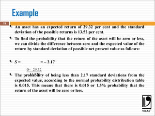
The document discusses key financial concepts including average and expected rates of return, risk measurement, and the calculation of variance and standard deviation. It explains the importance of normal distribution in evaluating investments and distinguishes between risk-averse, risk-neutral, and risk-seeking investor types. Additionally, it provides methodologies for calculating expected returns and probabilities related to asset returns.

1. LEARNING OBJECTIVES
 Discuss the concepts of average and expected rates of return.
 Define and measure risk for individual assets.
 Show the steps in the calculation of standard deviation and
variance of returns.
 Explain the concept of normal distribution and the importance
of standard deviation.
 Compute historical average return of securities and market
premium.
 Determine the relationship between risk and return.
 Highlight the difference between relevant and irrelevant risks.
1

2. Return on a Single Asset
 Total return = Dividend + Capital gain
2
 
1 1 0
1 0
1
1
0 0 0
Rate of return Dividend yield Capital gain yield
DIV
DIV P P
P P
R
P P P
 
 

  

3. Return on a Single Asset
21
.84
36.99
-6.73
1
0.81
-1
6.43
1
5.65
-27.45
40.94
1
2.83
2.93
-40
-30
-20
-10
0
10
20
30
40
50
1998 1999 2000 2001 2002 2003 2004 2005 2006 2007
Year
Total
Return
(%)
3
 Year-to-Year Total Returns on HUL Share

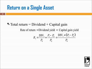
4. Average Rate of Return
 The average rate of return is the sum of the various
one-period rates of return divided by the number of
period.
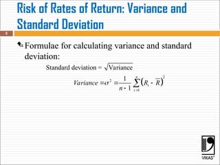
 Formula for the average rate of return is as follows:
4
1 2
=1
1 1
= [ ]
n
n t
t
R R R R R
n n
    


5. Risk of Rates of Return: Variance and
Standard Deviation
 Formulae for calculating variance and standard
deviation:
5
Standard deviation = Variance
 
2
2
1
1
1
n
t
t
Variance R R
n


  



6. 6
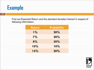
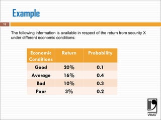
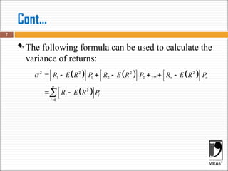
 The expected rate of return [E (R)] is the sum of the product of each outcome
(return) and its associated probability:
Expected Return : Incorporating Probabilities in
Estimates
Rates of Returns Under Various Economic Conditions
Returns and Probabilities

7. Cont…
 The following formula can be used to calculate the
variance of returns:
7
     
 
2 2 2 2
1 1 2 2
2
1
... n n
n
i
i
i
R E R P R E R P R E R P
R E R P


     
      
     
 
 
 


8. Example
8
i) Calculate Expected Return
ii) Variance
iii) Standard Deviation

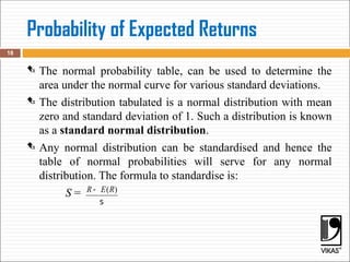
9. Return [R] Probability (P) R*P R-E (R-E)^2
9

10. Example
10
Find out Expected Return and the standard deviation thereof in respect of
following information:
Return Probability
1% 20%
7% 20%
8% 30%
10% 10%
15% 20%

11. 11

12. Example
12
The following information is available in respect of the return from security X
under different economic conditions:
Economic
Conditions
Return Probability
Good 20% 0.1
Average 16% 0.4
Bad 10% 0.3
Poor 3% 0.2

13. Expected Risk and Preference
 A risk-averse investor will choose among investments with
the equal rates of return, the investment with lowest standard
deviation and among investments with equal risk she would
prefer the one with higher return.
 A risk-neutral investor does not consider risk, and would
always prefer investments with higher returns.
 A risk-seeking investor likes investments with higher risk
irrespective of the rates of return. In reality, most (if not all)
investors are risk-averse.
13

14. Risk preferences
14

15. Normal Distribution and Standard Deviation
 In explaining the risk-return relationship, we
assume that returns are normally distributed.
 The spread of the normal distribution is
characterized by the standard deviation.
 Normal distribution is a population-based,
theoretical distribution.
15

16. 16
Normal distribution

17. Properties of a Normal Distribution
 The area under the curve sums to1.
 The curve reaches its maximum at the expected value (mean)
of the distribution and one-half of the area lies on either side
of the mean.
 Approximately 50 per cent of the area lies within ± 0.67
standard deviations of the expected value; about 68 per cent of
the area lies within ± 1.0 standard deviations of the expected
value; 95 per cent of the area lies within ± 1.96 standard
deviation of the expected value and 99 per cent of the area lies
within ± 3.0 standard deviations of the expected value.
17

18. Probability of Expected Returns
 The normal probability table, can be used to determine the
area under the normal curve for various standard deviations.
 The distribution tabulated is a normal distribution with mean
zero and standard deviation of 1. Such a distribution is known
as a standard normal distribution.
 Any normal distribution can be standardised and hence the
table of normal probabilities will serve for any normal
distribution. The formula to standardise is:
S =
18
( )
R E R
-
s

19. Example
 An asset has an expected return of 29.32 per cent and the standard
deviation of the possible returns is 13.52 per cent.
 To find the probability that the return of the asset will be zero or less,
we can divide the difference between zero and the expected value of the
return by standard deviation of possible net present value as follows:
 S = = – 2.17
 The probability of being less than 2.17 standard deviations from the
expected value, according to the normal probability distribution table
is 0.015. This means that there is 0.015 or 1.5% probability that the
return of the asset will be zero or less.
19
0 29.32
13.52
-