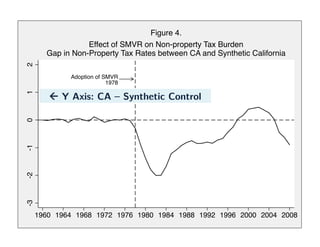
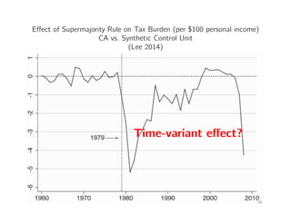
1) The document discusses a study analyzing the fiscal effects of constitutional supermajority requirements for raising taxes in U.S. states. 2) Using a synthetic control method, the study finds that California's non-property tax burden was $1.44 lower per $100 of personal income annually after adopting a 2/3 supermajority requirement in 1978, on average from 1979 to 2008. 3) Placebo tests indicate this effect is unique to California and not seen in other states, supporting a causal impact of the supermajority requirement on reducing taxes.

1. Fiscal Effects of the Constitutional
Supermajority Requirement for Raising
Taxes: Evidence from the U.S. States"
Soomi Lee"
Assistant Professor"
University of La Verne"
"
"
September 15, 2015"
Claremont Graduate University"
"
"

2. Supermajority vote requirement to raise/
impose taxes in state constitutions"
• Requires a supermajority to raise taxes instead of
a simple majority."
• A procedural rule to limit taxing power."
• One of the constitutional limits on taxes and
expenditure (TELs) "
• Sixteen states are currently under the requirement
(details vary): AZ, AR, CA, CO, DE, FL, KY, LA,
MI, MS, MO, NV, OK, OR, SD, (WA), (WI)."
1

3. Popular Reform Measure across States"
• Illinois (2005)"
• Maryland (2009)"
• New Hampshire (2011, 2013)"
• New York (2011) "
• Hawaii (2012)"
• Michigan (2012) "
• Indiana (2013)"
• North Dakota (2013)"

4. “[Legislators] have been too quick, in
the past, to try to solve our budget
problems by automatically looking at
tax increases” (Tom Cross (R) of
Illinois )"

5. Rationale & Opposition"
• Rationale: taming the Leviathan "
– Raise political transactions costs for a winning coalition
(Buchannan and Tullock 1962; Brennan and Buchannan
1978) "
– Restrain the growth of government"
– “Protect citizens against excessive taxation.” (WA 2015)"
• Cons: bad for fiscal outcome"
– Increase spending (paradox of SMVR, Lee et al. 2014)"
• Magnet of special interest & logrolling"
– Shift tax burdens onto minorities "
– Increase other levies not subject to SMVR "
– Raise borrowing costs"

6. Author(s) (Year)!
Sample
period !
Effects of SMVRs !
on Taxation!
Knight (2000)"
1963-1995
(IVFE)"
Reduces per capita average tax rate by
1.7 to 3.6%."
Beasley and Case
(2003)"
1960-1997" Reduces total taxes per capita by $52."
Bradbury and
Johnson (2006)"
1960-1997
(FE)"
No effect.!
Heckelman and
Dougherty (2010)"
1970-2008"
(Pooled
OLS)"
Reduces narrow-based tax rates "
No effect on broad based tax rates"
Lee, Borcherding,
and Kang (2013)"
1970-2007"
(IVFE)"
Increases total and income tax revenue"
Do They Work? "
Empirical Evidence: Major Studies on SMVR"

7. Challenges in Identifying Causality: "
Treatment of SMVR in Empirical Tests"
1. Heterogeneity of SMVR across states"
– Emergency provision: AR, CO, MO"
– AR: alcohol and sales taxes not subject to SMVR"
– MI: property taxes only"
– KY: odd-numbered years only"
2. Interpretations of % vote requirements"
– 75% requirement not necessarily more difficult than 67%."
– Arkansas 75% vs. California 67%"

8. 3. Changes over time"
– FL: 1971, 3/5 for corporate income tax; 1994, 2/3 for
tax increase; 1996, 2/3 voter approval for all tax & fee
increases"
– LA: 1921 for property taxes; 1974 all taxes"
4. Other inaccuracies"
– WA: SMVR suspended in 2001, 2005, and 2010"
– RI?"

9. Consequence: Violation of SUTVA"
(Stable Unit Treatment Value Assumption)"
• Multiple versions of treatment: the effect
for each state under SMVR will vary
depending on the version of SMVR."
• Consequence: The average causal effect will
not be relevant to every unit and “cannot be
used to draw causal inferences at the unit
level” (Holland 1986, 949). "

10. Empirical Strategy: Single Case Study
within Potential Outcome Framework"
• Potential outcome framework "
– Individual units have potential outcomes under
each treatment state: under SMVR and without
SMVR."
• Take a case to estimate the causal effect."

11. Case Selection: California"
• Passage of Proposition 13 (the People’s
Initiative to Limit Property Taxation) during
the 1978 tax revolt."
• It includes a 2/3 SMVR to raise any taxes."
• Frequently blamed for California’s budget
debacle."

12. Synthetic Control Method (SCM)"
(Abadie and Gardeazabal 2003; Abadie et al. 2010; Abadie et al. 2012)"
• Data-driven process to construct a suitable
comparison unit for California"
• Construct the unit by using the weighted average
of potential control states without SMVR (called
“donor pool”)"
• Use covariates to reproduce the trend of tax
burden of synthetic control before SMVR and
predict the behavior of tax burden of synthetic
control after the adoption of SMVR."

13. Data"
• State-level panel data from 1960 to 2008."
– Treatment year: 1978"
– 19 years of pre-intervention"
– 30 years of post-intervention"
• Donor pool: 33 states"
– Non-SMVR states only"
– Exclude Nebraska (unicameral)"

14. Outcome Variable"
• Non-property tax burden "
– Non-property state tax paid per $100 personal
income ($)"
– To eliminate the effect Prop.13 on property
taxes"

15. Adoption of SMVR
1978
2
4
6
8
10
12
1960 1964 1968 1972 1976 1980 1984 1988 1992 1996 2000 2004 2008
Total Taxes Non-Property Taxes Property Tax
Trend in California Tax Burden, 1960-2008
Tax Per $100 Personal Income
Figure 1.

16. Adoption of SMVR
1978
2
4
6
8
10
12
1960 1964 1968 1972 1976 1980 1984 1988 1992 1996 2000 2004 2008
Total Taxes Non-Property Taxes Property Tax
Trend in California Tax Burden, 1960-2008
Tax Per $100 Personal Income
Figure 1.

17. Adoption of SMVR
1978
2
4
6
8
10
12
1960 1964 1968 1972 1976 1980 1984 1988 1992 1996 2000 2004 2008
Total Taxes Non-Property Taxes Property Tax
Trend in California Tax Burden, 1960-2008
Tax Per $100 Personal Income
Figure 1.

18. Adoption of SMVR
1978
5
6
7
8
9
1960 1964 1968 1972 1976 1980 1984 1988 1992 1996 2000 2004 2008
California Donor Pool Average
Trend in Non-property Tax Burden
CA vs. Average of States without SMVR
Figure 2.

19. Adoption of SMVR
1978
5
6
7
8
9
1960 1964 1968 1972 1976 1980 1984 1988 1992 1996 2000 2004 2008
California Donor Pool Average
Trend in Non-property Tax Burden
CA vs. Average of States without SMVR
Figure 2.

20. Adoption of SMVR
1978
5
6
7
8
9
1960 1964 1968 1972 1976 1980 1984 1988 1992 1996 2000 2004 2008
California Donor Pool Average
Trend in Non-property Tax Burden
CA vs. Average of States without SMVR
Figure 2.

21. Predictor Variables"
• Per capita income, population, % child
population, unemployment rates, poverty
rates "
• % Democrats in the House, % Democrats
in the Senate, Governor’s party affiliation"

22. Adoption of SMVR
1978
5
6
7
8
9
1960 1964 1968 1972 1976 1980 1984 1988 1992 1996 2000 2004 2008
California Synthetic California
Trend in Non-property Tax Burden
CA vs. Synthetic California
Figure 3.
Synthetic CA
reproduces
pre-1978 tax
burden of CA well."

23. Adoption of SMVR
1978
5
6
7
8
9
1960 1964 1968 1972 1976 1980 1984 1988 1992 1996 2000 2004 2008
California Synthetic California
Trend in Non-property Tax Burden
CA vs. Synthetic California
Figure 3.
Synthetic CA
reproduces
pre-1978 tax
burden of CA well."

24. Adoption of SMVR
1978
-3
-2
-1
0
1
2
1960 1964 1968 1972 1976 1980 1984 1988 1992 1996 2000 2004 2008
Effect of SMVR on Non-property Tax Burden
Gap in Non-Property Tax Rates between CA and Synthetic California
Figure 4.
ß Y Axis: CA – Synthetic Control!

25. Adoption of SMVR
1978
-3
-2
-1
0
1
2
1960 1964 1968 1972 1976 1980 1984 1988 1992 1996 2000 2004 2008
Effect of SMVR on Non-property Tax Burden
Gap in Non-Property Tax Rates between CA and Synthetic California
Figure 4.
Average effect from 1979 to 2008: !
- 1.44 ($2005)!

26. Adoption of SMVR
1978
-3
-2
-1
0
1
2
1960 1964 1968 1972 1976 1980 1984 1988 1992 1996 2000 2004 2008
Effect of SMVR on Non-property Tax Burden
Gap in Non-Property Tax Rates between CA and Synthetic California
Figure 4.
Average effect from 1979 to 2008: !
- 1.44 ($2005)!
Average effect from 1979
to 1998: -1.05!

27. Placebo Studies"
Is this estimation credible?"
• Is the estimation of the tax burden a true
response to the adoption of SMVR in
California? Or is the estimate evaluated
entirely by chance?"
"

28. Placebo Studies 1"
• Apply SCM to states in the donor pool
states"
"

29. Adoption of SMVR
1978
California
Placebo States
-4
-3
-2
-1
0
1
2
3
4
1960 1964 1968 1972 1976 1980 1984 1988 1992 1996 2000 2004 2008
Effect of SMVR on Tax Burden in California and Placebo States
(States with Pre-1978 MSPE more than five times of CA's are excluded)
Figure 5.

30. Adoption of SMVR
1978
California
Placebo States
-4
-3
-2
-1
0
1
2
3
4
1960 1964 1968 1972 1976 1980 1984 1988 1992 1996 2000 2004 2008
Effect of SMVR on Tax Burden in California and Placebo States
(States with Pre-1978 MSPE more than five times of CA's are excluded)
Figure 5.
Unusually large
effect in California!

31. Adoption of SMVR
1978
California
Placebo States
-4
-3
-2
-1
0
1
2
3
4
1960 1964 1968 1972 1976 1980 1984 1988 1992 1996 2000 2004 2008
Effect of SMVR on Tax Burden in California and Placebo States
(States with Pre-1978 MSPE more than five times of CA's are excluded)
Figure 5.
Unusually large
effect in California!
Not Quite!

32. Placebo Studies 2"
• Reassign SMVR in the dataset to a
year different than 1978 (California)"

33. Placebo SMVR Adoption
1974
Real SMVR Adoption
1978
5
6
7
8
9
1960 1964 1968 1972 1976 1980 1984 1988 1992 1996 2000 2004 2008
California Synthetic California
Placebo Adoption Year: 1974
Trend in Non-Property Tax Burden
Figure 6.
No discernable effect
after a placebo
treatment"

34. Conclusion"
• Since the adoption of SMVR through 2008,
Californians have had lower non property tax
burden than what they would have without
SMVR. "
– 73 cents per $100 personal income per year"
• The adoption of SMVR had a bigger immediate
effect in curbing tax burden, but the effect
decayed over time. "

35. Effect of Supermajority Rule on Tax Burden (per $100 personal income) "
CA vs. Synthetic Control Unit "
(Lee 2014)"
Time-variant effect?!
34

36. How Governments Cope with Supermajority
Rule to Raise Taxes?"
• Possible state actions"
1. Circumvent the rule "
2. Do not circumvent the rule"
1. Use referenda to raise taxes"
2. Undermine the rule to eliminate the limits on taxing power"
• Assumptions"
– Balanced budget "
– Increasing demand for public programs (budget
pathology, Block 2008)"
35

37. Circumvention hypothesis "
(Kiewiet and Szakaly 1996)"
• States circumvent constitutional constraints on
taxing and spending power. "
• Applied to many other constitutional limits: debt
limits, expenditure limits, balanced budget
requirements."
• State behaviors to cope with the supermajority
rule to raise taxes are not well understood."
36

38. 1. Circumvent "
• Raise taxes and fees/surcharges that are
not subject to the supermajority rule"
– Both opponents and supports of the rule claim this."
– CA Proposition 26 (2010)"
• State-enterprise exemptions"
– California Chamber of Commerce, et al. v. California Air
Resources Board, 2013. (green house gas allowances)!
– TABOR Foundation v. Colorado Bridge Enterprise, 2014.
(bridge safety surcharge)!
37

39. 2. Do not circumvent"
• Increase taxes through initiatives and referendum"
• Often temporary and renewed multiple times"
• Example: California Gov. Gerry Brown’s
Proposition 30 in 2012."
38

40. 3. Undermine the rule"
• Nevada"
– Guinn v. Legislature of Nev. (2002)"
• Washington"
– Legislative tampering (2001, renewed twice)"
– League of Education Voters v. Washington State
(2013, the court ruled that the supermajority rule is
unconstitutional under the state constitution)"
39

41. Expected Effects of "
Supermajority Rule to Raise Taxes"
" No circumvention" Circumvention"
Tax"
Reduces tax burden initially,
but the effect decays. "
(time-varying effect)"
Reduces taxes initially and the
effect lasts over time. "
(no time-varying effects)"
Fee" No significant change"
Fees should increase after the
rule adoption and the effect
lasts over time "
40

42. Data and Method"
• Use the natural variation in the timing of the rule
adoption: state-level panel data from 1960-2008"
• Use fixed-effects model to account for unobserved
heterogeneity with robust standard errors"
• Alaska & Nebraska excluded among the non-
supermajority states"
41

43. Variables"
• Dependent variables:"
– Tax burden (per $1,000 personal income)"
– Fee burden (per $1,000 personal income)"
• Key variables:"
– Supermajority rule in effect"
– # years passed after the rule adoption (curvilinear)"
42

44. • Demographic variables: Population (log), Per capita
income ($2010 thousands), % dependent population"
• Political variables: Governor’s party affiliation, %
Democrats in the lower house, % Democrats in the
upper house, divided government, Citizen ideology,
Government ideology"
• Institutional variables: expenditure limit,
appropriation limit, revenue limit (no limit as a
reference category), Presence of legislative term
limit"
Control Variables"
43

45. Question 1:"
Is the effect of supermajority rules"
time-varying? "
44

46. Effects of Supermajority Rule on "
Taxes (per $1,000 personal income)"
OLS" FE"
(1)" (2)" (3)" (4)"
Supermajority rule"
(dummy variable) "
-1.205" 2.791" -3.954**" .742"
(3.907)" (3.235)" (1.610)" (1.34)"
Years "
(#years after adoption)"
-.384" -.767**"
(.457)" (.297)"
Years2"
.003" .017**"
(.01)" (.007)"
N! 2256" 2256" 2256" 2256"
R2! .843" .847" .510" .522"
Notes: State clustered standard errors are in parenthesis. All models include
control variables and year dummies. * p<.1; ** p<.05. ***p<.01. "
45

47. Effects of Supermajority Rule on "
Taxes (per $1,000 personal income)"
OLS" FE"
(1)" (2)" (3)" (4)"
Supermajority rule"
(dummy variable) "
-1.205" 2.791" -3.954**" .742"
(3.907)" (3.235)" (1.610)" (1.34)"
Years "
(#years after adoption)"
-.384" -.767**"
(.457)" (.297)"
Years2"
.003" .017**"
(.01)" (.007)"
N! 2256" 2256" 2256" 2256"
R2! .843" .847" .510" .522"
Notes: State clustered standard errors are in parenthesis. All models include
control variables and year dummies. * p<.1; ** p<.05. ***p<.01. "
46

48. Effects of Supermajority Rule on "
Taxes (per $1,000 personal income)"
OLS" FE"
(1)" (2)" (3)" (4)"
Supermajority rule"
(dummy variable) "
-1.205" 2.791" -3.954**" .742"
(3.907)" (3.235)" (1.610)" (1.34)"
Years "
(#years after adoption)"
-.384" -.767**"
(.457)" (.297)"
Years2"
.003" .017**"
(.01)" (.007)"
N! 2256" 2256" 2256" 2256"
R2! .843" .847" .510" .522"
Notes: State clustered standard errors are in parenthesis. All models include
control variables and year dummies. * p<.1; ** p<.05. ***p<.01. "
47

49. Question 2:"
Do states under the supermajority
requirement significantly increase fees?"
48

50. 49
Effects of Supermajority Rule on "
Fees (per $1,000 personal income)"
OLS" FE"
(1)" (2)" (3)" (4)"
Supermajority rule"
(dummy variable) "
1.700" -1.289" .461" -.889"
(3.312)" (1.423)" (1.911)" (1.019)"
Years "
(#years after adoption)"
.659**" .260"
(.292)" (.242)"
Years2"
-.022**" -.008**"
(.007)" (.005)"
N! 2256" 2256" 2256" 2256"
R2! .609" .624" .690" .691"
Notes: State clustered standard errors are in parenthesis. All models include
control variables and year dummies. * p<.1; ** p<.05. ***p<.01. "

51. 50
Effects of Supermajority Rule on "
Fees (per $1,000 personal income)"
OLS" FE"
(1)" (2)" (3)" (4)"
Supermajority rule"
(dummy variable) "
1.700" -1.289" .461" -.889"
(3.312)" (1.423)" (1.911)" (1.019)"
Years "
(#years after adoption)"
.659**" .260"
(.292)" (.242)"
Years2"
-.022**" -.008**"
(.007)" (.005)"
N! 2256" 2256" 2256" 2256"
R2! .609" .624" .690" .691"
Notes: State clustered standard errors are in parenthesis. All models include
control variables and year dummies. * p<.1; ** p<.05. ***p<.01. "

52. 51
Effects of Supermajority Rule on "
Fees (per $1,000 personal income)"
OLS" FE"
(1)" (2)" (3)" (4)"
Supermajority rule"
(dummy variable) "
1.700" -1.289" .461" -.889"
(3.312)" (1.423)" (1.911)" (1.019)"
Years "
(#years after adoption)"
.659**" .260"
(.292)" (.242)"
Years2"
-.022**" -.008**"
(.007)" (.005)"
N! 2256" 2256" 2256" 2256"
R2! .609" .624" .690" .691"
Notes: State clustered standard errors are in parenthesis. All models include
control variables and year dummies. * p<.1; ** p<.05. ***p<.01. "

53. 5
10
15
Fees
and
charges
Per
$1,000
personal
income
1960 1970 1980 1990 2000 2010
Supermajority states Non-supermajority states
Trend of Fee Burden by Supermajority Status:
1960-2008 "
52

54. Expected Effects of Supermajority Rule to Raise Taxes"
" No circumvention" Circumvention"
Tax"
Reduces tax burden initially,
but the effect decays. "
(time-varying effect)"
Reduces taxes initially and the
effect lasts over time. "
(no time-varying effects)"
Fee" No significant change"
Fees should increase after the
rule adoption and the effect
lasts over time "
53

55. Robustness Checks"
• Different sample time periods"
– Knight (2000) & Lee et al. (2014)"
• Different coding to account for
heterogeneity of supermajority rules"
– MI: non-supermajority"
– FL: 1971 v. 1994"
– WA: non-supermajority since 2001"
54

56. Conclusion"
• Supermajority rule has a time-varying effect on tax
burden."
• Supermajority rule reduces tax burden in the short
run but increases it in the long run (the long run
magnitude is small). "
• There is no evidence that states increase fees to
raise revenue."
• Results support neither the Buchanan-Tullock
conjecture nor the circumvention hypothesis. "
55

57. Thank You."

58. Empirical Model (SCM)!
• Goal of the empirical model:"
where i=states, t=year, Y=observed outcome under SMVR,
YN=observed outcome without treatment, S=existence of
SMVR; α=effect of SMVR. "
• To estimate α for California (i=1)"
• Estimate the effect of adoption of SMVR:"
where =observed outcome for CA."
• Need to estimate the unobserved average tax rates of
California in the absence of SMVR, :"
Yit = Yit
N
+αitSit, !
α1t = Y1t
I
−Y1t
N
= Y1t
I
−Y1t
N
. !
Y1t
N
= δt +θt Zi + λt µi + εit, !
Y1t
I
!
Y1t
N
!

59. • A vector of weights: ,"
Where j=states in the donor pool."
• The vector of weights "
minimizes pre-intervention characteristics "
between the tax rate of California and "
that of its synthetic control. "
• Weighted average of control states:"
"
• Estimate the effect of SMVR adoption on average tax rate
in California:"
W = (w2,…,wJ+1 ′
) !
W*
= (w2
*
,,wJ+1
*
′
) !
wj
*
Yjt = δt +θt wj
*
j
j=2
J+1
∑ Zj + λt wj
*
j=2
J+1
∑ µj + wj
*
εjt.
j=2
J+1
∑ !
α̂1t = Y1t − wj
*
Yjt
j=1
J+1
∑ . !

60. Predictor Balance!
California
Donor
pool
average
Variables
Observed
SyntheBc
Log
of
populaBon
16.778
15.014
14.693
%
PopulaBon
under
age
of
18
0.333
0.354
0.350
Real
income
($2005
current)
23157
21536
19045
Unemployment
rate
(%
civilian)
7.109
6.281
5.463
Poverty
rate
(%,
individual)
10.75
9.857
12.259
%
Democrats
in
State
House
0.596
0.618
0.602
%
Democrats
in
State
Senate
0.595
0.59
0.585
Governor’s
party
affiliaBon
0.555
0.598
0.611

61. Unit Weights!
State
Weight
Alaska
.127
Hawaii
.205
Indiana
.166
MassachuseZs
.087
New
Jersey
.103
New
York
.095
Ohio
.108
Texas
.109

62. CA
0
1
2
3
4
5
6
7
8
9
10
11
#
States
0 5 10 15 20 25 30 35 40 45
Panel A: From 1979 to 1988
CA
0
1
2
3
4
5
6
7
8
9
10
11
#
States
0 5 10 15 20 25 30 35
Panel B: From 1979 to 2008
Figure 7.
Ratio of Post-SMVR MSPE and Pre-SMVR MSPE

63. 62
Fixed Effect Model with an Instrumental Variable"
Tax" Fee"
1st stage" 2nd stage" 1st stage" 2nd stage"
Supermajority rule"
(dummy variable) "
66.877*" -20.81"
(38.37)" (18.35)"
Years "
(#years after adoption)"
-7.908*" 2.411"
(.4.146)" (1.983)"
Years2"
.207*" .065"
(.110)" (.053)"
Initiative"
.049**" .049**"
(.025)" (.025)"
1st stage F statistic! 4.03**" 4.03**"
N! 2256" 2256"
R2! .691" .546"
Notes: State clustered standard errors are in parenthesis. All models
include control variables and year dummies. * p<.1; ** p<.05.
***p<.01. "