Download to read offline
![A&A 546, A105 (2012) Astronomy
DOI: 10.1051/0004-6361/201117166 &
c ESO 2012 Astrophysics
The hypergiant HR 8752 evolving through the yellow
evolutionary void ,
H. Nieuwenhuijzen1 , C. De Jager1,2 , I. Kolka3 , G. Israelian4 , A. Lobel5 , E. Zsoldos6 , A. Maeder7 , and G. Meynet7
1
SRON Laboratory for Space Research, Sorbonnelaan 2, 3584 CA Utrecht, The Netherlands
e-mail: h.nieuwenhuijzen@sron.nl; h.nieuwenhuijzen@xs4all.nl
2
NIOZ, Royal Netherlands Institute for Sea Research, PO Box 59, Den Burg, The Netherlands
e-mail: cdej@kpnplanet.nl
3
Tartu Observatory, 61602 Tõravere, Estonia
e-mail: indrek@aai.ee
4
Instituto de Astrofisica de Canarias, via Lactea s/n, 38200 La Laguna, Tenerife, Spain
e-mail: gil@iac.es
5
Royal Observatory of Belgium, Ringlaan 3, 1180 Brussels, Belgium
e-mail: alobel@sdf.lonestar.org; Alex.Lobel@oma.be
6
Konkoly Observatory, PO Box 67, 1525 Budapest, Hungary
e-mail: zsoldos@konkoly.hu
7
Observatoire de Genève, 1290 Sauverny, Switzerland
e-mail: [Andre.Maeder;Georges.Meynet]@unige.ch
Received 30 April 2011 / Accepted 13 March 2012
ABSTRACT
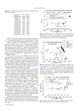
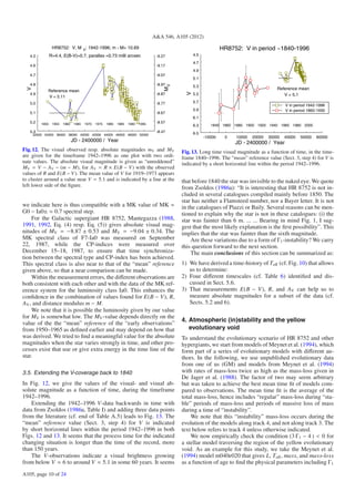
Context. We study the time history of the yellow hypergiant HR 8752 based on high-resolution spectra (1973–2005), the observed
MK spectral classification data, B − V- and V-observations (1918–1996) and yet earlier V-observations (1840–1918).
Aims. Our local thermal equilibrium analysis of the spectra yields accurate values of the effective temperature (T eff ), the accelera-
tion of gravity (g), and the turbulent velocity (vt ) for 26 spectra. The standard deviations average are 82 K for T eff , 0.23 for log g,
and 1.1 km s−1 for vt .
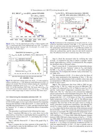
Methods. A comparison of B− V observations, MK spectral types, and T eff -data yields E(B− V), “intrinsic” B− V, T eff , absorption AV ,
and the bolometric correction BC. With the additional information from simultaneous values of B − V, V, and an estimated value of R,
the ratio of specific absorption to the interstellar absorption parameter E(B − V), the “unreddened” bolometric magnitude mbol,0 can
be determined. With Hipparcos distance measurements of HR 8752, the absolute bolometric magnitude Mbol,0 can be determined.
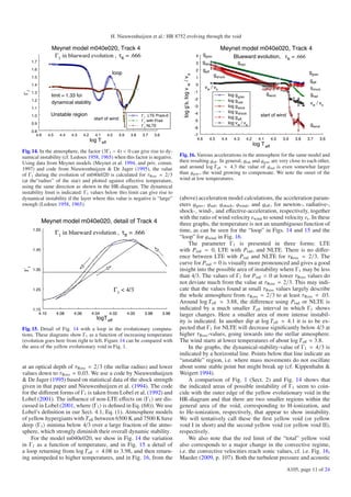
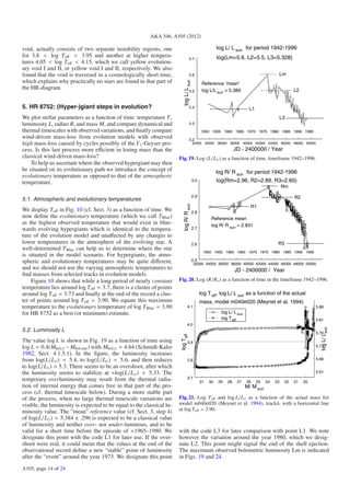
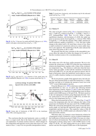
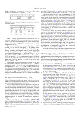
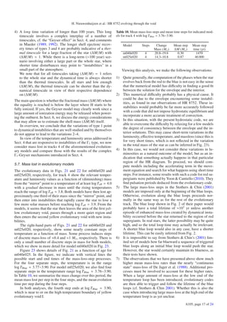
Results. Over the period of our study, the value of T eff gradually increased during a number of downward excursions that were ob-
servable over the period of sufficient time coverage. These observations, together with those of the effective acceleration g and the
turbulent velocity vt , suggest that the star underwent a number of successive gas ejections. During each ejection, a pseudo photosphere
was produced of increasingly smaller g and higher vt values. After the dispersion into space of the ejected shells and after the restruc-
turing of the star’s atmosphere, a hotter and more compact photosphere became visible. From the B − V and V observations, the basic
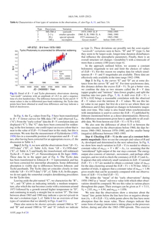
stellar parameters, T eff , log M/M , log L/L , and log R/R are determined for each of the observational points. The results show the
variation in these basic stellar parameters over the past near-century.
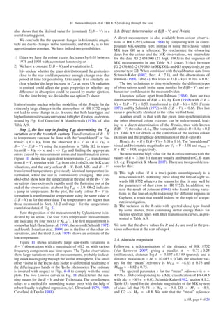
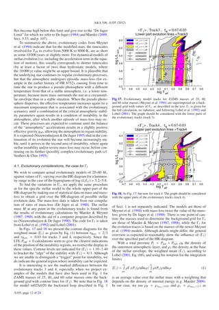
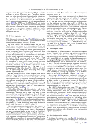
Conclusions. We show that the atmospheric instability region in the HR-diagram that we baptize the yellow evolutionary void actually
consists of two parts. We claim that the present observations show that HR 8752 is presently climbing out of the “first” instability
region and that it is on its way to stability, but in the course of its future evolution it still has to go through the second potential unstable
region.
Key words. stars: atmospheres – stars: evolution – supergiants – stars: mass-loss – stars: fundamental parameters –
stars: variables: S Doradus
1. Introduction 1.1. The yellow hypergiants; HR 8752 in the literature
We summarize in this section the status of knowledge on The star HR 8752 is a member of a group of half a dozen massive
HR 8752 and the evolution of hypergiants and succinctly review stars, with zero age main sequence (ZAMS) masses of 20–40 or
the aims of this research. even more solar masses, the yellow hypergiants. Another well-
studied member is ρ Cas (Lobel et al. 1992, 1994, 1998, 2003;
Appendix A is available in electronic form at
http://www.aanda.org Israelian et al. 1999; Gorlova et al. 2006). These are sites of
Tables A.x and B.x are available in electronic form at the CDS via heavy mass-loss, which is sometimes episodic. The individual
anonymous ftp to stars undergo large variations in temperature. These variations
cdsarc.u-strasbg.fr (130.79.128.5) or via are the visible atmospheric manifestations of changes that are
http://cdsarc.u-strasbg.fr/viz-bin/qcat?J/A+A/546/A105, only semi-coupled to the star, underlying its (pseudo-) photo-
and at the external site http://www.aai.ee/HR~8752 sphere. The evolutionary changes of the underlying star have a
Article published by EDP Sciences A105, page 1 of 24](https://image.slidesharecdn.com/2012-hr8752-void-crossing-121018103441-phpapp01/85/2012-hr8752-void-crossing-1-320.jpg)
![A&A 546, A105 (2012) Astronomy
DOI: 10.1051/0004-6361/201117166 &
c ESO 2012 Astrophysics
The hypergiant HR 8752 evolving through the yellow
evolutionary void ,
H. Nieuwenhuijzen1 , C. De Jager1,2 , I. Kolka3 , G. Israelian4 , A. Lobel5 , E. Zsoldos6 , A. Maeder7 , and G. Meynet7
1
SRON Laboratory for Space Research, Sorbonnelaan 2, 3584 CA Utrecht, The Netherlands
e-mail: h.nieuwenhuijzen@sron.nl; h.nieuwenhuijzen@xs4all.nl
2
NIOZ, Royal Netherlands Institute for Sea Research, PO Box 59, Den Burg, The Netherlands
e-mail: cdej@kpnplanet.nl
3
Tartu Observatory, 61602 Tõravere, Estonia
e-mail: indrek@aai.ee
4
Instituto de Astrofisica de Canarias, via Lactea s/n, 38200 La Laguna, Tenerife, Spain
e-mail: gil@iac.es
5
Royal Observatory of Belgium, Ringlaan 3, 1180 Brussels, Belgium
e-mail: alobel@sdf.lonestar.org; Alex.Lobel@oma.be
6
Konkoly Observatory, PO Box 67, 1525 Budapest, Hungary
e-mail: zsoldos@konkoly.hu
7
Observatoire de Genève, 1290 Sauverny, Switzerland
e-mail: [Andre.Maeder;Georges.Meynet]@unige.ch
Received 30 April 2011 / Accepted 13 March 2012
ABSTRACT
Context. We study the time history of the yellow hypergiant HR 8752 based on high-resolution spectra (1973–2005), the observed
MK spectral classification data, B − V- and V-observations (1918–1996) and yet earlier V-observations (1840–1918).
Aims. Our local thermal equilibrium analysis of the spectra yields accurate values of the effective temperature (T eff ), the accelera-
tion of gravity (g), and the turbulent velocity (vt ) for 26 spectra. The standard deviations average are 82 K for T eff , 0.23 for log g,
and 1.1 km s−1 for vt .
Methods. A comparison of B− V observations, MK spectral types, and T eff -data yields E(B− V), “intrinsic” B− V, T eff , absorption AV ,
and the bolometric correction BC. With the additional information from simultaneous values of B − V, V, and an estimated value of R,
the ratio of specific absorption to the interstellar absorption parameter E(B − V), the “unreddened” bolometric magnitude mbol,0 can
be determined. With Hipparcos distance measurements of HR 8752, the absolute bolometric magnitude Mbol,0 can be determined.
Results. Over the period of our study, the value of T eff gradually increased during a number of downward excursions that were ob-
servable over the period of sufficient time coverage. These observations, together with those of the effective acceleration g and the
turbulent velocity vt , suggest that the star underwent a number of successive gas ejections. During each ejection, a pseudo photosphere
was produced of increasingly smaller g and higher vt values. After the dispersion into space of the ejected shells and after the restruc-
turing of the star’s atmosphere, a hotter and more compact photosphere became visible. From the B − V and V observations, the basic
stellar parameters, T eff , log M/M , log L/L , and log R/R are determined for each of the observational points. The results show the
variation in these basic stellar parameters over the past near-century.
Conclusions. We show that the atmospheric instability region in the HR-diagram that we baptize the yellow evolutionary void actually
consists of two parts. We claim that the present observations show that HR 8752 is presently climbing out of the “first” instability
region and that it is on its way to stability, but in the course of its future evolution it still has to go through the second potential unstable
region.
Key words. stars: atmospheres – stars: evolution – supergiants – stars: mass-loss – stars: fundamental parameters –
stars: variables: S Doradus
1. Introduction 1.1. The yellow hypergiants; HR 8752 in the literature
We summarize in this section the status of knowledge on The star HR 8752 is a member of a group of half a dozen massive
HR 8752 and the evolution of hypergiants and succinctly review stars, with zero age main sequence (ZAMS) masses of 20–40 or
the aims of this research. even more solar masses, the yellow hypergiants. Another well-
studied member is ρ Cas (Lobel et al. 1992, 1994, 1998, 2003;
Appendix A is available in electronic form at
http://www.aanda.org Israelian et al. 1999; Gorlova et al. 2006). These are sites of
Tables A.x and B.x are available in electronic form at the CDS via heavy mass-loss, which is sometimes episodic. The individual
anonymous ftp to stars undergo large variations in temperature. These variations
cdsarc.u-strasbg.fr (130.79.128.5) or via are the visible atmospheric manifestations of changes that are
http://cdsarc.u-strasbg.fr/viz-bin/qcat?J/A+A/546/A105, only semi-coupled to the star, underlying its (pseudo-) photo-
and at the external site http://www.aai.ee/HR~8752 sphere. The evolutionary changes of the underlying star have a
Article published by EDP Sciences A105, page 1 of 24](https://image.slidesharecdn.com/2012-hr8752-void-crossing-121018103441-phpapp01/75/2012-hr8752-void-crossing-1-2048.jpg)
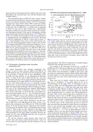

This study examines the evolution of the yellow hypergiant star HR 8752 over nearly a century based on spectroscopic observations and photometry. The star underwent successive gas ejections, seen as downward excursions in effective temperature. During each ejection, a pseudo-photosphere formed with lower gravity and higher turbulence. After the ejected shells dispersed, a hotter, more compact photosphere emerged. Analysis of observations shows variation over time in the star's effective temperature, luminosity, radius, and mass, suggesting it is evolving away from an unstable region in the HR diagram known as the "yellow evolutionary void."


