https://workshopmanuals.co/ Workshopmanualsco provides workshop repair manuals just like the professional repair shops use. We provide an instant manual download after purchase. These detail manuals have parts list, wiring diagrams, maintenance information and everything the DIY car enthusiast will need. We have repair guides for all the top auto manufacturers. (Alfa Romero, Aston Martin, Audi, Bentley, BMW, Chevrolet, Citroen, Daihatsu, Ford, GMC, Honda, Hummer, Lexus, Mercedes-Benz, Renault, Tesla, Toyota, Vauxhall, Volvo, VW & so much more!
Clinical Trials Versus Health Outcomes Research: SAS/STAT Versus SAS Enterpri...cambridgeWD
Clinical trials and health outcomes research differ in important ways that impact statistical modeling approaches. Clinical trials typically use homogeneous samples and focus on a single endpoint, while health outcomes data is heterogeneous with multiple endpoints. Predictive modeling techniques used in health outcomes research, like those in SAS Enterprise Miner, are better suited than traditional methods as they can handle complex real-world data without strong assumptions and more accurately predict rare events. Validation of models on separate test data is also important for generalizing results.
Clinical Trials Versus Health Outcomes Research: SAS/STAT Versus SAS Enterpri...cambridgeWD
This document discusses the differences between clinical trials and health outcomes research. Clinical trials use homogeneous samples, surrogate endpoints, and focus on a single outcome. They are also typically underpowered for rare events. Health outcomes research uses heterogeneous data from the general population to examine multiple real endpoints simultaneously. It has larger samples and data that allow analysis of rare occurrences. Predictive modeling is better suited than traditional statistical methods for analyzing heterogeneous health outcomes data due to relaxed assumptions like normality.
This study evaluated the performance of bootstrap confidence intervals for estimating slope coefficients in Model II regression with three or more variables. Simulation studies were conducted for different correlation structures between variables, sampling from both normal and lognormal distributions. The results showed that bootstrap intervals provided less than the nominal 95% coverage. Scenarios with strong relationships between variables produced better coverage, while scenarios with weaker relationships and bias produced poorer coverage, even with larger sample sizes. Future work could explore additional scenarios and alternative interval methods to improve accuracy of confidence intervals in Model II regression.
A Cox model is a statistical technique used to analyze survival data with several explanatory variables. It allows estimation of the hazard or risk of an event like death for an individual based on prognostic factors. A Cox model expresses the hazard as an exponential function of the explanatory variables. Interpreting a Cox model involves examining the regression coefficients - a positive coefficient means a higher hazard/worse prognosis, while a negative coefficient implies a better prognosis. The model from a study of melanoma patients' survival found age and cancer type increased hazard, while male sex decreased it, and interferon treatment did not significantly impact survival.
The document discusses using R to analyze data from the NHANES dataset. Density estimation revealed the age variable was bimodal. Linear discriminant analysis and classification trees were used to predict class variables with mixed results. Support vector machines better predicted insulin use with a polynomial kernel than a linear kernel.
large data set is not available for some disease such as Brain Tumor. This and part2 presentation shows how to find "Actionable solution from a difficult cancer dataset
Life Expectancy Estimate with Bivariate Weibull Distribution using Archimedea...CSCJournals
Archimedean copulas are used to construct bivariate Weibull distributions. Co-movement structures of variables are analyzed through the copulas, where the tail dependence between the variables is explored with more flexibility. Based on the distance between the copula distribution and its empirical version, a copula that may best fit data is selected. With extra computing costs, the adequacy of the copula chosen is then assessed. When multiple myeloma data are considered, it is found that relationship between survival time of a patient and the hemoglobin level is well described by the Clayton copula. The bivariate Weibull distribution constructed by the copula is used to estimate value at risk from which we investigate the anticipated longest life expectancy of a patient with the disease over the treatment period.
Use Proportional Hazards Regression Method To Analyze The Survival of Patient...Waqas Tariq
The Kaplan Meier method is used to analyze data based on the survival time. In this paper used Kaplan Meier procedure and Cox regression with these objectives. The objectives are finding the percentage of survival at any time of interest, comparing the survival time of two studied groups and examining the effect of continuous covariates with the relationship between an event and possible explanatory variables. The variables (Age, Gender, Weight, Drinking, Smoking, District, Employer, Blood Group) are used to study the survival patients with cancer stomach. The data in this study taken from Hiwa/Hospital in Sualamaniyah governorate during the period of (48) months starting from (1/1/2010) to (31/12/2013) .After Appling the Cox model and achieve the hypothesis we estimated the parameters of the model by using (Partial Likelihood) method and then test the variables by using (Wald test) the result show that the variables age and weight are influential at the survival of time.
Clinical Trials Versus Health Outcomes Research: SAS/STAT Versus SAS Enterpri...cambridgeWD
Clinical trials and health outcomes research differ in important ways that impact statistical modeling approaches. Clinical trials typically use homogeneous samples and focus on a single endpoint, while health outcomes data is heterogeneous with multiple endpoints. Predictive modeling techniques used in health outcomes research, like those in SAS Enterprise Miner, are better suited than traditional methods as they can handle complex real-world data without strong assumptions and more accurately predict rare events. Validation of models on separate test data is also important for generalizing results.
Clinical Trials Versus Health Outcomes Research: SAS/STAT Versus SAS Enterpri...cambridgeWD
This document discusses the differences between clinical trials and health outcomes research. Clinical trials use homogeneous samples, surrogate endpoints, and focus on a single outcome. They are also typically underpowered for rare events. Health outcomes research uses heterogeneous data from the general population to examine multiple real endpoints simultaneously. It has larger samples and data that allow analysis of rare occurrences. Predictive modeling is better suited than traditional statistical methods for analyzing heterogeneous health outcomes data due to relaxed assumptions like normality.
This study evaluated the performance of bootstrap confidence intervals for estimating slope coefficients in Model II regression with three or more variables. Simulation studies were conducted for different correlation structures between variables, sampling from both normal and lognormal distributions. The results showed that bootstrap intervals provided less than the nominal 95% coverage. Scenarios with strong relationships between variables produced better coverage, while scenarios with weaker relationships and bias produced poorer coverage, even with larger sample sizes. Future work could explore additional scenarios and alternative interval methods to improve accuracy of confidence intervals in Model II regression.
A Cox model is a statistical technique used to analyze survival data with several explanatory variables. It allows estimation of the hazard or risk of an event like death for an individual based on prognostic factors. A Cox model expresses the hazard as an exponential function of the explanatory variables. Interpreting a Cox model involves examining the regression coefficients - a positive coefficient means a higher hazard/worse prognosis, while a negative coefficient implies a better prognosis. The model from a study of melanoma patients' survival found age and cancer type increased hazard, while male sex decreased it, and interferon treatment did not significantly impact survival.
The document discusses using R to analyze data from the NHANES dataset. Density estimation revealed the age variable was bimodal. Linear discriminant analysis and classification trees were used to predict class variables with mixed results. Support vector machines better predicted insulin use with a polynomial kernel than a linear kernel.
large data set is not available for some disease such as Brain Tumor. This and part2 presentation shows how to find "Actionable solution from a difficult cancer dataset
Life Expectancy Estimate with Bivariate Weibull Distribution using Archimedea...CSCJournals
Archimedean copulas are used to construct bivariate Weibull distributions. Co-movement structures of variables are analyzed through the copulas, where the tail dependence between the variables is explored with more flexibility. Based on the distance between the copula distribution and its empirical version, a copula that may best fit data is selected. With extra computing costs, the adequacy of the copula chosen is then assessed. When multiple myeloma data are considered, it is found that relationship between survival time of a patient and the hemoglobin level is well described by the Clayton copula. The bivariate Weibull distribution constructed by the copula is used to estimate value at risk from which we investigate the anticipated longest life expectancy of a patient with the disease over the treatment period.
Use Proportional Hazards Regression Method To Analyze The Survival of Patient...Waqas Tariq
The Kaplan Meier method is used to analyze data based on the survival time. In this paper used Kaplan Meier procedure and Cox regression with these objectives. The objectives are finding the percentage of survival at any time of interest, comparing the survival time of two studied groups and examining the effect of continuous covariates with the relationship between an event and possible explanatory variables. The variables (Age, Gender, Weight, Drinking, Smoking, District, Employer, Blood Group) are used to study the survival patients with cancer stomach. The data in this study taken from Hiwa/Hospital in Sualamaniyah governorate during the period of (48) months starting from (1/1/2010) to (31/12/2013) .After Appling the Cox model and achieve the hypothesis we estimated the parameters of the model by using (Partial Likelihood) method and then test the variables by using (Wald test) the result show that the variables age and weight are influential at the survival of time.
This document discusses different methods for analyzing survival data in clinical trials, including Kaplan-Meier survival analysis and restricted mean survival time (RMST) analysis. It reviews literature on survival analysis concepts and applications. The document also notes limitations of Kaplan-Meier analysis when data does not satisfy proportional hazards assumptions or when patients are lost to follow up. RMST is presented as an alternative to estimate mean survival times without these limitations. The document then applies different survival analysis methods to a dataset to compare results.
Probability Models for Estimating Haplotype Frequencies and Bayesian Survival...Université de Dschang
M. Kum Cletus Kwa a soutenu une thèse de Doctorat/Phd en mathématiques ce 14 juin 2016 à l'Université de Dschang. Le jury lui a décerné à l'issue des échanges la mention très honorable.
This document discusses the concept of equifinality in complex environmental systems modeling. Equifinality refers to the idea that there are many different model structures and parameter sets that can produce similar and acceptable results when modeling system behavior. The generalized likelihood uncertainty estimation (GLUE) methodology is described as a way to account for equifinality by using ensembles of behavioral models weighted by their likelihood to estimate prediction uncertainties. An example application to rainfall-runoff modeling is used to illustrate the GLUE methodology.
Clinical Trial Simulation to Evaluate the Pharmacokinetics of an Abuse-Deterr...Loan Pham
A CTS was performed to estimate the sample size and optimal plasma sampling times that sufficiently characterize the PK parameters (CL, Vd) from a single dose of an abuse-deterrent (AD) opioid in pediatric subjects.
Confidence Intervals in the Life Sciences PresentationNamesS.docxmaxinesmith73660
Confidence Intervals in the Life Sciences Presentation
Names
Statistics for the Life Sciences STAT/167
Date
Fahad M. Gohar M.S.A.S
1
Conservation Biology of Bears
Normal Distribution
Standard normal distribution
Confidence Interval
Population Mean
Population Variance
Confidence Level
Point Estimate
Critical Value
Margin of Error
Welcome to the presentation on Confidence Intervals of Conservation Biology on Bears.
The team will define normal distribution and use an example of variables why this is important. A standard and normal distribution is discussed as well as the difference between standard and other normal distributions. Confidence interval will be defined and how it is used in Conservation Biology and Bears. We will learn how a confidence interval helps researchers estimate of population mean and population variance. The presenters defined a point estimate and try to explain how a point estimate found from a confidence interval. Confidence level is defined and a short explanation of confidence level is related to the confidence interval. Lastly, a critical value and margin of error are explained with examples from the Statdisk.
2
Normal Distribution
A normal distribution is one which has the mean, median, and mode are the same and the standard deviations are apart from the mean in the probabilities that go with the empirical rule. Not all data has the measures of central tendency, since some data sets may not have one unique value which occurs more than once. But every data set has a mean and median. The mean is only good with interval and ratio data, while the median can be used with interval, ratio and ordinal data. Mean is used when they're a lot of outliers, and median is used when there are few.
The normal distribution is continuous, and has only two parameters - mean and variance. The mean can be any positive number and variance can be any positive number (can't be negative - the mean and variance), so there are an infinite number of normal distributions. You want your data to represent the population distribution because when you make claims from the distribution of the sample you took, you want it to represent the whole entire population.
Some examples in the business world: Some industries which use normal distributions are pharmaceutical companies. They model the average blood pressure through normal distributions, and can make medicine which will help majority of the people with high blood pressure. A company can also model its average time to create something using the normal distribution. Several statistics can be calculated with the normal distribution, and hypothesis tests can be done with the normal distribution which models the average time.
Our chosen life science is BEARS. The age of the bears can be modeled by normal distributions and it is important to monitor since that tells us the average age of the bear, and can tell us a lot about the population. If the mean is high and the standard deviatio.
The error threshold is a limit on the number of base pairs a self-replicating molecule can have before mutations destroy the information. It arises because during replication, each base pair has a chance of mutating. If the molecule exceeds a critical size, mutations overwhelm the information. Eigen's paradox notes this limits early molecules to around 100 bases, but genes need thousands, creating a chicken-and-egg problem of which came first. Proposed solutions include correlated molecules enhancing each other's replication accuracy, or mutation rates being lower than initially believed, allowing longer sequences.
The document summarizes a simulation study that examined the effects of using raw scores versus IRT-derived scores when operationalizing latent constructs in moderated multiple regression analyses. The study found that using raw scores can inflate Type 1 error rates for interaction terms under conditions of assessment inappropriateness. However, rescaling the scores using the Graded Response Model, a polytomous IRT model, mitigated these effects. The study supports the idea that IRT scores provide a more robust metric than raw scores in moderated regression analyses, especially under suboptimal assessment conditions.
This document summarizes a proposed novel method for crossover operators in genetic algorithms called the sigmoid crossover. It begins by discussing issues with existing crossover operators that use a fixed crossover probability, such as populations converging too quickly and getting stuck in local optima. It then proposes using a sigmoid probability distribution for crossover instead of a fixed value. This distribution is based on the genetic distance between chromosomes, with chromosomes that are more different having a higher chance of crossover. The document provides mathematical background on sigmoid functions and genetic distance. It then describes the proposed sigmoid crossover method and how it modifies the typical genetic algorithm crossover procedure by replacing the fixed probability with one based on genetic distance. This is intended to help preserve genetic diversity in the population and give a
This document compares several dimension reduction techniques for survival analysis when there are many covariates: principal component analysis (PCA), partial least squares (PLS), and three variants of random matrices (RM) based on Johnson-Lindenstrauss embeddings. It simulates 5,000 datasets using the accelerated failure time model and determines the total bias error and mean-squared error between the true and estimated survivor curves for each method. The results indicate that PCA outperforms PLS, the RMs are comparable, and the RMs outdo both PCA and PLS.
1. The document proposes a formalism to utilize clinically available MRI imaging data for early detection of resistance to targeted cancer therapies.
2. By extracting tumor growth parameters from serial MRI scans, mathematical models can be used to predict future tumor growth and identify signs of resistance earlier than current methods.
3. Simulated data is used to determine the number and frequency of scans needed to reliably extract parameters and detect resistance under different levels of initial resistance and sampling intervals.
- Multinomial logistic regression predicts categorical membership in a dependent variable based on multiple independent variables. It is an extension of binary logistic regression that allows for more than two categories.
- Careful data analysis including checking for outliers and multicollinearity is important. A minimum sample size of 10 cases per independent variable is recommended.
- Multinomial logistic regression does not assume normality, linearity or homoscedasticity like discriminant function analysis does, making it more flexible and commonly used. It does assume independence between dependent variable categories.
This document presents a methodology for modeling mortality rates across Canadian provinces. It reviews literature on single and multi-population mortality models. Mortality indices from 1921-2009 for 9 provinces are analyzed using unit root tests and the Johansen cointegration test, which finds common trends among the indices. Vector error correction (VECM) and vector autoregressive (VAR) models are estimated and show better fit for female mortality. The models are used to project and forecast mortality indices 50 years into the future and to price annuities for cohorts from 1960-2000, with VECM producing more accurate pricing. In conclusion, mortality trends are declining across provinces with common factors, and VECM performs better than VAR or ARIMA models
Application of Semiparametric Non-Linear Model on Panel Data with Very Small ...IOSRJM
-This research work investigated the behaviour of a new semiparametric non-linear (SPNL) model on
a set of panel data with very small time point (T = 1). The SPNL model incorporates the relationship between
individual independent variable and unobserved heterogeneity variable. Five different estimation techniques
namely; Least Square (LS), Generalized Method of Moments (GMM), Continuously Updating (CU), Empirical
Likelihood (EL) and Exponential Tilting (ET) Estimators were employed for the estimation; for the purpose of
modelling the metrical response variable non-linearly on a set of independent variables. The performances of
these estimators on the SPNL model were examined for different parameters in the model using the Least
Square Error (LSE), Mean Absolute Error (MAE) and Median Absolute Error (MedAE) criteria at the lowest
time point (T = 1). The results showed that the ET estimator which provided the least errors of estimation is
relatively more efficient for the proposed model than any of the other estimators considered. It is therefore
recommended that the ET estimator should be employed to estimate the SPNL model for panel data with very
small time point.
Logistic Loglogistic With Long Term Survivors For Split Population ModelWaqas Tariq
Split population models are also known as mixture model . The data used in this paper is Stanford Heart Transplant data. Survival times of potential heart transplant recipients from their date of acceptance into the Stanford Heart Transplant program [3]. This set consists of the survival times, in days, uncensored and censored for the 103 patients and with 3 covariates are considered Ages of patients in years, Surgery and Transplant, failure for these individuals is death. Covariate methods have been examined quite extensively in the context of parametric survival models for which the distribution of the survival times depends on the vector of covariates associated with each individual. See [6] for approaches which accommodate censoring and covariates in the ordinary exponential model for survival. Currently, such mixture models with immunes and covariates are in use in many areas such as medicine and criminology. See for examples [4][5][7]. In our formulation, the covariates are incorporated into a split loglogistic model by allowing the proportion of ultimate failures and the rate of failure to depend on the covariates and the unknown parameter vectors via logistic model. Within this setup, we provide simple sufficient conditions for the existence, consistency, and asymptotic normality of a maximum likelihood estimator for the parameters involved. As an application of this theory, the likelihood ratio test for a difference in immune proportions is shown to have an asymptotic chi-square distribution. These results allow immediate practical applications on the covariates and also provide some insight into the assumptions on the covariates and the censoring mechanism that are likely to be needed in practice. Our models and analysis are described in section 5.
2019/ 10/ 11 Originality Report
iginalityReport/ultra?attemptId=929ba456-7401-4cb2-8818-df87061d712f&course_id=_65931_1&includeDeleted=true&print=true&download=true… 1/3
%33
SafeAssign Originality Report
(Current Semester - الفصل الحالي)HCM-506: Appli… • Turnitin Plagiarism Checker
%33Total Score: Medium risk
MOHAMMED ALAHMARI
Submission UUID: b770c976-29f1-45b0-6be2-a23c9f149d8d
Total Number of Repo…
1
Highest Match
33 %
133333.docx
Average Match
33 %
Submitted on
10/11/19
10:36 AM GMT+3
Average Word Count
362
Highest: 133333.docx
%33Attachment 1
Global database (3)
Student paper Student paper Student paper
Top sources (3)
Excluded sources (0)
View Originality Report - Old Design
Word Count: 362
133333.docx
3 2 1
3 Student paper 2 Student paper 1 Student paper
https://lms.seu.edu.sa/webapps/mdb-sa-BBLEARN/originalityReport?attemptId=929ba456-7401-4cb2-8818-df87061d712f&course_id=_65931_1&download=true&includeDeleted=true&print=true&force=true
2019/ 10/ 11 Originality Report
iginalityReport/ultra?attemptId=929ba456-7401-4cb2-8818-df87061d712f&course_id=_65931_1&includeDeleted=true&print=true&download=true… 2/3
Source Matches (6)
Student paper
86%
Student paper
98%
Student paper
96%
Student paper
92%
Module 13
Name: Date:
Kaplan-Meier plots: The goal is to estimate a population survival curve from a sample. i) If every patient is followed until
death, the curve may be estimated simply by computing the fraction surviving at each time. ii) However, in most studies
patients tend to drop out, become lost to follow-up, move away, etc. iii) A Kaplan-Meier analysis allows estimation of
survival over time, even when points drop out or are studied for different lengths of time.
H0 The survival time is not related to the patient treatment group. (Null Hypothesis) H1 The survival time is related to the
patient treatment group. (Alternative Hypothesis)
Baseline Survivor Function (at predictor means)... 0.0000 0.8465 1.0000 0.3114
Interpretation of the curve: Vertical axis represents estimated probability of survival for a hypothetical cohort, not actual %
surviving. • Precision of estimates depends on # observations; therefore, estimates at left-hand side are more precise than at
right-hand side (because of small #’s due to deaths and dropouts). • Curves may give the impression that a given event
occurs more frequently early than late, because of high survival rate and large # people at beginning
Yes, Kaplan-Meier survival curves prognostic indicator of UCEC because it can be generated by selecting the cancer type,
survival type and protein(s) of interest. This technique may also be used for breast, colon and other cancers because its a
statistical technique which gives proper result of survival data of the patients undergone cancer or other treatment.
References Hazra, A., & Gogtay, N. (2016). Biostatistics series module 6: Correlation and linear regression. Indian Journal of
Dermatology, 61(6), 593-601. Retr.
Heteroscedasticity occurs when the variance of the error terms in a regression model are not constant, but instead vary depending on the values of the independent variables. While ordinary least squares estimators remain unbiased, their standard errors may be incorrect under heteroscedasticity. This means that confidence intervals and hypothesis tests based on the usual standard errors are unreliable and can lead to misleading conclusions.
This document discusses key concepts in statistical analysis:
1) Error bars represent the variability in data and can show the range or standard deviation. The standard deviation summarizes how data values are spread around the mean, with 68% of values within one standard deviation.
2) The standard deviation is useful for comparing means and spreads between samples. Larger differences in means and standard deviations between samples indicate they are less likely from the same population.
3) A t-test measures the overlap between two data sets and determines if their differences are statistically significant or likely due to chance. A significance level of 5% is commonly used, below which the null hypothesis that sets are the same is rejected.
This study analyzed the correlation between osteoclast survival and function in patients with either high or low metal exposure from metal-on-metal hip replacements. Sixteen patients were divided into two groups based on their cobalt and chromium serum levels. Four variables related to osteoclast number, function, and activity were measured and compared between the groups. Statistical analysis found little evidence of a difference in osteoclast number and activity between groups, but some evidence of a difference in functional osteoclasts and osteoclastic resorption. Overall, the results did not provide sufficient evidence to conclude a difference in osteoclast survival and function between high and low metal exposure patients due to small sample size and wide variability in some measures.
This paper is a methodological exercices presenting the results obtained from the estimation of the growth convergence equation using different methodologies.
A dynamic balanced panel data is estimated using: OLS, WithinGroup, HsiaoAnderson, First Difference, GMM with endogenous and GMM with predetermined instruments. An unbalanced panel is also realized for OLS, WG and FD.
Results are discused in light of Monte Carlo studies.
Electrical Testing Lab Services in Dubai.pptxsandeepmetsuae
An electrical testing lab in Dubai plays a crucial role in ensuring the safety and efficiency of electrical systems across various industries. Equipped with state-of-the-art technology and staffed by experienced professionals, these labs conduct comprehensive tests on electrical components, systems, and installations.
Material Testing Lab Services in Dubai.pptxsandeepmetsuae
Dubai is home to numerous advanced material testing labs, offering state-of-the-art facilities for a wide range of industries. These labs provide critical services such as mechanical testing, chemical analysis, and non-destructive testing, ensuring the quality and durability of materials used in construction, aerospace, and manufacturing.
Check CNIC Information | +447490809237 | CNIC Details Checkerownerdetailssim
Whatsapp Number For Paid Service:
+447490809237
The CNIC Information System is a comprehensive database managed by the National Database and Registration Authority (NADRA) of Pakistan. It serves as the primary source of identification for Pakistani citizens and residents, containing vital information such as name, date of birth, address, and biometric data.
nadra cnic details
cnic details with picture
cnic details
how to check cnic details with picture
check cnic details
cnic details online
cnic number details
how to check cnic details
how to check cnic number details online
cnic detail by cnic number
how can i check my cnic details
nadra cnic detail check
number details with cnic
how to check cnic details online
cnic details with picture online
cnic sim details
check cnic details online
how can i check my cnic details online
how to check sim detail on cnic
how to check sim details on cnic
check cnic number details online in pakistan
cnic check details
cnic full detail
how can i check cnic details
my cnic details
pakistan cnic number details
cnic details finder
cnic details pakistan
how to check cnic details by mobile number
how to check nadra cnic details
online cnic details check
pakistani cnic details
sim cnic detail
sim details on cnic
check detail with cnic number
check mobilink sim number customer detail and cnic number
find cnic details
how to check cnic details pakistan
how to check my cnic details online
my cnic card details
bank account details by cnic number
check cnic number details
cnic details by number
cnic number sim detail
details through cnic number
how to check my cnic details
sim number details by cnic
cnic details with mother name
fbr cnic details
how to check father cnic number details online
mobile number cnic details online
cnic detail with cnic number
online check cnic detail
verify cnic details
check online cnic detail
cnic pic details
get details from cnic number
how can i check my cnic details through cnic number
how to find cnic details
how to find cnic number details
pakistan cnic details
pakistan cnic details online
check cnic detail by cnic number
check detail by cnic number
check sim details by cnic
cnic card details
details from cnic number
find details by cnic number
how to get details from cnic number
mobile number detail with name and cnic in pakistan
can i check my cnic details online
check cnic card details
check cnic details nadra
check cnic details pakistan
check cnic number details online
check cnic sim details
check details of cnic number
check my cnic details
check nadra cnic details
check nadra cnic full detail and print copy
check online cnic id card verification and detail bio data
check sim details on cnic
check your cnic details online
cnic code details
cnic details check online
cnic details online check
cnic details through sms
cnic details with father name
cnic details with mobile number
cnic details with name
cnic details with picture online pakistan
cnic no detail
cnic number check details
Material Testing Lab Services in Dubai.pdfsandeepmetsuae
Dubai is home to numerous advanced material testing labs, offering state-of-the-art facilities for a wide range of industries. These labs provide critical services such as mechanical testing, chemical analysis, and non-destructive testing, ensuring the quality and durability of materials used in construction, aerospace, and manufacturing.
Whatsapp Number For Paid Services:
+447490809237
Find Sim owner details easily with our Live Tracker. You will get accurate and instant sim information with number. Whether, you are looking for Nadra Sim Ownership details or location we are here to serve you.
Are you in need of quick and reliable access to SIM ownership details and other essential information for Pakistani telecommunications customers? Look no further!
Our live tracker is providing you with up-to-date SIM database information within seconds. Gone are the days of waiting for official sources to provide this data, as our service offers instant access to SIM ownership details, equivalent to information obtained from official sources but without the long wait times.
With just basic internet skills and a stable connection, you can conveniently access Pakistani SIM data, including owner details for 2024. Whether you need to verify phone number details, check SIM information, or access mobile number information online, our platform has you covered. Save time and effort by using our service today!
Sim Tracker – Free Sim Data 2024
Here are the some tools that are free to use like sim tracker, sim database checker , sim owner details , and also vehicle owner details and if you want our premium or paid services then you can contact us on whatsapp.
How to Verify the Number of SIM Cards Registered under your CNIC?
If you want to check how many SIM cards are registered under your name, you can do it easily. Just go to your mobile network provider’s website or app. Look for the feature called “SIM Ownership CNIC Tracker.” Then, type in your CNIC number correctly. After you submit it, the system will show you a list of all the SIM cards registered under your name. It will tell you which ones are active (in use) and which ones are inactive (not in use). Check this list carefully to see if there are any SIM cards you don’t need anymore. If you find any inactive ones, you can remove them to make room for new ones. This is helpful if you’re trying to add a new SIM card but all the slots are full. If you have any questions or problems with the registered SIM cards, you can contact your mobile network provider’s customer support for help.. By doing this, you can manage your SIM cards better and make sure you’re using your slots efficiently.
What information does live tracker provide for CNIC numbers?
SimOwnerDetails.online offers a comprehensive range of NADRA sim owner details for CNIC numbers. This includes the holder’s name, address, and a complete list of mobile numbers registered under the CNIC. Users can access detailed information about each registered SIM, facilitating better management and security of their telecommunications accounts.
What Sim information does SimOwnerDetails.online provide for SIM card numbers?
#sim owner details
#sim owner details pakistan
#nadra sim owner details
#sim owner details by number
#sim owner details online
#sim owner details apk
#sim owner details app
Whatsapp Number: +447490809237
sim owner details
sim owner details pakistan
nadra sim owner details
sim owner details by number
sim owner details online
sim owner details apk
sim owner details app
sim owner details online check pakistan
pak sim data sim owner details
zong sim owner details
check sim owner details
how to check sim owner details in pakistan
find sim owner details in pakistan
mobile sim owner details
how to check sim owner details
sim card owner details
sim card owner details online
sim owner details with name and address
track sim card owner details online
jio sim owner details
sim owner details software
check sim card owner details
find sim owner details
how to check airtel sim owner details
how to check sim card owner details
how to find a sim owner details
how to find sim owner details
how to know sim card owner details
how to know sim owner details
idea sim card owner details online
sim card owner details app
sim card owner details software
sim owner name details
ufone sim owner details
00923456435194 sim owner detail
ap to know the sim owners details
check sim number owner details
find out details of owner of sim card
finding sim registration owner details
full details of sim card owner pakistan
how to check my sim owner details
how to check owner detail through sim
how to check owner details of a sim
how to check owner details of jaz sim
how to check sim owner details who tease people
how to check sim owner name and detail warid
how to chek owner details of sim
how to find a sim owner details pakista
how to find a sim owner details pakistan
how to find sim card owner details in pakistan
how to get details of others sim owner in pakistan
how to trace a sim owner details pakistan
idea sim card owner details
iran sim details of owner
iran sim details of owner website
mobile phone number details sim owner name address
mobile phone number details sim owner name address location
online sim owner details.pakistan
pakistan prepaid sim owner details
pakistan sim owner details
phone number details sim owner name address location
search sim card owner and details using apk
sim card owner details app for pakistan
sim detail check online owner
sim details online by number owner name
sim number all details with owner name
sim number all details with owner name id card
sim owner call details online
sim owner details by contact number
sim owner details online with name and address
sim owner name full details
Best Web Development Frameworks in 2024growthgrids
Best Web Development Frameworks: In 2024, the landscape of web development frameworks is diverse, with different frameworks excelling in various aspects such as 1. React, 2. Jquery, 3. MySQL, and 4. ASP.NET. With a strategic blend of manual testing and cutting-edge automated tools, we guarantee a flawless user experience. Partner with Growth Grids and elevate your software quality to new heights.
Contact Us :-
Email: [business@growthgrids.com]
Phone: [+91-9773356002]
Website : https://growthgrids.com
Webroot antivirus helps with online security. Use reliable security software to protect your devices from attacks, providing online security and quiet mind when using technology for business or work.
The Fraud Examiner’s Report –
What the Certified Fraud Examiner Should Know
Being a Virtual Training Paper presented at the Association of Certified Fraud Examiners (ACFE) Port Harcourt Chapter Anti-Fraud Training on July 29, 2023.
A Dojo Training PPT focuses on hands-on, immersive learning to enhance skills and knowledge. It emphasizes practical experience, fostering continuous improvement and collaboration within your team to achieve excellence.
#1 Call Girls in Islamabad || 03274100048 || Quick Booking at Affordable Priceownerdetailssim
Islamabad Call Girls Services – Available 24/7
One of the most educated and reliable Call Girls in Islamabad. They only work with real guys who want to enjoy the company of our high-class, sexy call girls with love and respect. Our call girls have enough experience to know how to make their guests happy at that time. Of course, we’re known for our genuine hospitality.
Our stylish Independent Islamabad call girls are available 24 hours a day, seven days a week. People who work for our agency will make you feel right at home as soon as you meet them. You’ll feel like you’re at a real Call Girl agency in Islamabad.
Our guests come back repeatedly, and no matter what megacity they visit, they always contact us to talk about the nightlife. If you’re in a big city by yourself and getting sexy in a hotel room. Our girls are so well-trained that they can go to a club, a party, or a DJ night with you and make you feel unforgettable.
Our VIP call girls are dedicated to their jobs and look forward to giving you a great experience and ensuring you’re delighted. We are quick at getting new gifts, which is why our customers love us so much. Before, you saw our girls’ portfolios and hot pictures, which made you want to do anything. Book your stay in Islamabad right now by calling.
Special Moments with Islamabad Call Girls
Customers are surprised by how satisfying, inspiring, and powerful Islamabad Call Girl’s minutes are, which makes them love her even more. Our agency’s name in the market is due to our excellent call girls, who keep clients coming back for life.
As a Call Girl service in Islamabad, Islamabad Nights Call Girl has been helping a wide range of clients for a long time. His work makes the value of the business easy to understand, appealing, and beautiful. The only thing that makes the firm successful is its dedication to giving clients excellent customer service.
The terms and conditions of the Islamabad Call Girls service are standard. Kids under 18 can’t get help from this government because it doesn’t want them; they have to be at least 18 years old. His agency only gives the power to mature people travelling with real sidekicks.
The people who work for this office are trained, responsible, and prepared for their jobs. They don’t like other Call Girls who only want money in exchange for giving clients beds. They serve both inside and outside people.
Ready to Meet Islamabad Call Girls Now!
You don’t need to wait. We’ll send hot Call Girls to your house if you call us. It’s easy for these young, pretty women to make guys happy.
No need to worry about how they treat you because they are all very friendly and work for a company. They know how to make every guy happy.
#call girls in islamabad #islamabad call girls #call girl in islamabad #islamabad call girl
How Live-In Care Benefits Chronic Disease Management.pdfKenWaterhouse
Explore how live-in care can significantly benefit chronic disease management, enhancing the quality of life for those affected and providing peace of mind for their families.
Stay updated on Siddhivinayak Temple events and timings in Houston, TX. Join our spiritual and community gatherings. Visit us now! gaurisiddhivinayak.org
Landscape Architect Melbourne specializes in designing stunning, sustainable outdoor spaces that blend creativity with functionality. From lush gardens to innovative urban landscapes, they transform environments into aesthetically pleasing, eco-friendly havens. Their expertise ensures each project harmonizes with its surroundings, enhancing Melbourne's unique urban character while promoting environmental stewardship.
Top 10 Challenges That Every Web Designer Face on A Daily Basis.pptxe-Definers Technology
In today’s fast-moving digital world, building websites is super important for how well a business does online. But, because things keep changing with technology and what people expect, teams who make websites often run into big problems. These problems can slow down their work and stop them from making really good websites. Let us see what the best website designers in Delhi have to say –
https://www.edtech.in/services/website-designing-development-company-delhi.htm
How Can I Apply in India (2024) for a US B1/B2 Visa Renewal?usaisofficial
Are your US visas current? Though it will soon expire, I’m not sure what to do. We will assist you in getting a fresh US visa and being protected. The procedures and conditions for renewing a US B1/B2 visa can grab your attention. This blog article will cover everything you need to know regarding the US B1/B2 visa renewal in India in 2024. Alternatively, do you have to show up for an interview? Right now, the US B1/B2 visa waiting period in India is what?
How Long Does Vinyl Siding Last and What Impacts Its Life Expectancy?Alexa Bale
The majority of siding industry insiders assert that vinyl has a 20–40-year lifespan. Although this lifetime indicates an increase over earlier siding types, the average life expectancy is heavily dependent on outside factors. Vinyl siding needs to be carefully maintained, especially after a weather event. Dive into ppt to know How Long Does Vinyl Siding Last and What Impacts Its Life Expectancy.
How Long Does Vinyl Siding Last and What Impacts Its Life Expectancy?
13roafis (1).pdf
1. 570
Size at 50% maturity (l50%) is com-
monly evaluated for wild popula-
tions as a point of biological refer-
ence (see Table 1). To estimate l50%,
a sample of organisms known to
have just reached sexual maturity
could be available and their arith-
metic mean size can be used as an
estimator. However, the sample
needed to obtain such a design-
based estimator (Smith, 1990) for
wild populations might be too ex-
pensive and would involve time-con-
suming histological procedures.
Fisheries biologists prefer to con-
ceive size at first maturity as the
average size at which 50% of the
individuals are mature. With this
conception, the estimator is not
based on a sampling design but on
a model of the relation between
body size and the number of indi-
viduals that are mature from a to-
tal number at each of many size in-
tervals. The variance of a design-
based estimator is determined by
sampling design (Thompson, 1992).
The variance of a model-based esti-
mator is not as easily obtained. A
sample of published works in the
fisheries literature provides a mea-
sure of the frequency with which
Estimation of size at sexual maturity:
an evaluation of analytical and
resampling procedures
Rubén Roa
Departamento de Oceanografía
Universidad de Concepción
Casilla 160-C, Concepción, Chile
E-mail address: rroa@udec.cl
Billy Ernst
School of Fisheries, WH-10
University of Washington, Seattle, Washington 98195
Fabián Tapia
Departamento de Oceanografía
Universidad de Concepción
Casilla 160-C, Concepción, Chile
Manuscript accepted 28 August 1998.
Fish. Bull. 97:570–580 (1999).
Abstract.–Size at 50% maturity is
commonly evaluated for wild popula-
tions, but the uncertainty involved in
such computation has been frequently
overlooked in the application to marine
fisheries. Here we evaluate three pro-
cedures to obtain a confidence interval
for size at 50% maturity, and in gen-
eral for P% maturity: Fieller’s analyti-
cal method, nonparametric bootstrap,
and a Monte Carlo algorithm. The three
methods are compared in estimating
size at 50% maturity (l50%) by using
simulated data from an age-structured
population, with von Bertalanffy
growth and constant natural mortality,
for sample sizes of 500 to 10,000 indi-
viduals. Performance was assessed by
using four criteria: 1) the proportion of
times that the confidence interval did
contain the true and known size at 50%
maturity, 2) bias in estimating l50%, 3)
length and 4) shape of the confidence
interval around l50%. Judging from cri-
teria 2–4, the three methods performed
equally well, but in criterion 1, the
Monte Carlo method outperformed the
bootstrap and Fieller methods with a
frequency remaining very close to the
nominal 95% at all sample sizes. The
Monte Carlo method was also robust to
variations in natural mortality rate
(M), although with lengthier and more
asymmetric confidence intervals as M
increased. This method was applied to
two sets of real data. First, we used
data from the squat lobster Pleuron-
codes monodon with several levels of
proportion mature, so that a confidence
interval for the whole maturity curve
could be outlined. Second, we compared
two samples of the anchovy Engraulis
ringens from different localities in cen-
tral Chile to test the hypothesis that
they differed in size at 50% maturity
and concluded that they were not sta-
tistically different.
statistical uncertainty of the model-
based l50% is ignored (Table 1). In
this work, we show three alterna-
tive procedures: an analytical
method derived from generalized
linear models (McCullagh and
Nelder, 1989), nonparametric boot-
strap (Efron and Tibshirani, 1993),
and a Monte Carlo algorithm devel-
oped in our study. We show by simu-
lation the behavior of the three
methods for sample sizes of 500 to
10,000 individuals, concluding that
they are similar in terms of bias,
length, and shape of confidence inter-
vals but that the Monte Carlo method
outperforms the other two methods
in percentage of times that the confi-
dence interval contains the true pa-
rameter, which remained close to the
nominal 95% at all sample sizes.
The problem
In regression analysis, we are usu-
ally interested in assigning confi-
dence bounds to the response vari-
able at specified levels of the pre-
dictor variable. However, in matu-
rity modeling the attention is
turned to the converse problem of
2. 571
Roa et al.: Estimation of size at sexual maturity
Table 1
An example of published analyses on size at maturity in crustacean and fish populations. CW = carapace width; CL = carapace
length; TL = total length; m = males; f = females; g = gonadal maturity; m = morphometric maturity.
Paper
Somerton
(1980)
Campbell
and
Robinson
(1983)
Somerton
and
MacIntosh
(1983)
Campbell
and Eagles
(1983)
Somerton
and Otto
(1986)
Gaertner
and Laloé
(1986)
Comeau
and Conan
(1992)
Armstrong
et al. (1982)
Lovrich
and
Vinuesa
(1993)
Roa (1993a)
González-
Gurriarán
and Freire
(1994)
Species
Paralithodes
camtschatica
Chionoecetes bairdi
Homarus americanus
Paralithodes platypus
Cancer irroratus
Lithodes aequispina
Geryon maritae
Chionoecetes opilio
Lophius americanus
(Pisces: Lophiiformes)
Paralomis granulosa
Pleuroncodes
monodon
Necora puber
Fitting method
Weighted nonlinear
least-squares
Nonlinear
least-squares
Weighted nonlinear
least-squares
Nonlinear
least-squares
Weighted nonlinear
least-squares
Nonlinear
least-squares
Nonlinear
least-squares
Linear regression of
Prop. Mature (arcsine-
square root trans-
formed)onTotalLength
Probit
Maximum likelihood
Maximum likelihood
l50% (mm)
102.8 (CL, m)
101.9 (CL, f)
114.7 (CW, m)
108.1 (CL, f)
92.5 (CL, f)
78.5 (CL, f)
80.6 (CL, f)
96.3 (CL, f)
93.7 (CL, f)
87.4 (CL, f)
62.0 (CW, m)
49.0 (CL, f)
97.7 (CL, f)
99.0 (CL, f)
110.7 (CL, f)
92.0 (CL, m)
107.0 (CL, m)
130.0 (CL, f)
82.8 (CL, f)
34.2 (CW, m)
368.9 (TL, m)
458.3 (TL, f)
50.2 (CL, m)g
60.6 (CL, f)g
57.0 (CL, m)m
66.5 (CL, f)
27.2 (CL, f)
54.8 CW, m)g
49.8 (CW, f)g
53.3 (CW, m)m
52.3 (CW, f)m
CI 95%
Not reported
Not reported
Not reported
—
—
—
79.4–82.6
95.7–96.9
92.9–94.5
86.4–88.4
—
—
Values not reported
—
—
—
—
—
58.3–62.9
53.9–60.1
63.4–69.5
24.2–30.2
—
—
—
—
CI estimation method
Random partition of data
into subsets and computa-
tion of var (l50%) among the
N independent estimates
of l50%
—
—
—
Random partition of data
into subsets and computa-
tion of var (l50%) among the
N independent estimates
of l50%
—
—
Bootstrap samples were
drawn from the original
data set for obtaining in-
dependent estimates of
l50%, and then computing
var(l50%) among them.
Confidence regions for the
parameters of a logistic
function were computed.
—
—
—
—
Not reported
Not reported
Not reported
Ratio of parameter esti-
mates confidence limits
—
—
—
—
setting a confidence interval for the size at which a
fixed proportion of individuals in a population are
sexually mature. That is, we need a procedure for
estimating uncertainty in the predictor variable be-
cause management decisions are framed in terms of
body size, and hence the uncertainty in estimation
3. 572 Fishery Bulletin 97(3), 1999
must be transferred to this variable. The first part
of the problem is the selection of the maturity model.
The available data consist of size (normally length)
and maturity status, which will be assumed to take
only two values: mature or immature. The predictor
variable is continuous and the response variable is
dichotomous. With such variables, model errors dis-
tribute binomially. Welch and Foucher (1988) recog-
nized this aspect of modeling maturity and showed
an efficient procedure based on the principle of maxi-
mum likelihood that takes advantage of the binomial
nature of the errors.
For dichotomous data modeled as a function of a
continuous variable, the following simple logistic
function is a consequence of the assumption of a lin-
ear relationship between the logit link function and
a single predictor variable (Shanubhogue and Gore,
1987; Hosmer and Lemeshow, 1989; McCullagh and
Nelder, 1989):
P l
e l
( ) ,
=
+ +
α
β β
1 0 1
(1)
where P(l) = proportion mature at size l; and
α, β0, and β1 = asymptote, intercept, and slope pa-
rameters, respectively (see also Eq. 3).
The estimates of these parameters, given a data set,
are chosen from the point at which the product of
binomial mass functions of all data points (the likeli-
hood of the data under the model) is a maximum, or
equivalently when the negative of the log likelihood
− = − ( )+ − −
( )
[ ]
∑
l( , ) ( )ln ( ) ( )ln ( )
,
α β β
0 1 1
h P l n h P l
l l l
l
(2)
is a minimum,
where h = the number of mature individuals; and
n = sample size at l;
P(l) = Eq. 1; and
where a constant term that does not affect the esti-
mation is omitted.
Given the nonlinear nature of normal equations,
the minimum is found by an iteration algorithm. The
parameters estimated by minimizing Equation 2 are
maximum likelihood estimates (MLE). In practical
situations, the logistic model may be modified from
its original form to allow more biological reality
(Welch and Foucher, 1988).
The result from fitting the model (Eq. 1) to the data
by using the objective in Equation 2, is a vector of
parameter estimates and a covariance matrix, which
represents the uncertainty associated to them. With
these results, we may undertake the converse prob-
lem of estimating size at fixed P% maturity, which
takes the form
l
P
P% ln .
= −
−
1 1
1
1
0
1
β
β
β
(3)
In Equation 3 it is assumed that the asymptote pa-
rameter (α) from Equation 1 is fixed at 1. This as-
sumption is justified on the basis of several published
works on size at maturity, showing that all individu-
als were mature above a given size during the repro-
ductive season (Table 1). Furthermore, if β̂ 0 and β̂ 1
are MLE of β0 and β1 and they are used to compute
lP% from Equation 3, then l̂% is also MLE. We show
below three procedures to perform this task and then
test them by generating data from Monte Carlo simu-
lation of the age-size structure and maturity progres-
sion of individuals of a hypothetical population.
Analytical estimation
The logistic model in Equation 1 belongs to a class of
generalized linear models studied by McCullagh and
Nelder (1989). These authors consider the problem
of building approximate confidence intervals for the
level of the predictor variable that gives rise to a fixed
proportion in the response variable. They suggest the
use of Fieller’s (1944) theorem, according to which
the linear combination
β β
0 1 0 0
+ − =
l g P
P% ( ) , (4)
where lP% = the value of the predictor variable for a
fixed proportion; and g(P0)=ln(P0/(1–P0)) (the logit
link function) is approximately normal with mean
zero and analytical variance given by
v l l l
P P P
2
0 0 1
2
1
2
( ) var( ˆ ) cov( ˆ , ˆ ) var( ˆ ).
% % %
= + +
β β β β (5)
The 100(1–α)% confidence interval is the set of val-
ues defined by
1
1
0 0 2
ˆ
ˆ ( ) ( ) ,
/ %
β
β
− + ±
( )
g P z v l
a P
(6)
where zα/2 = a quantile of the normal distribution.
Other link functions like probit, common in the field
of toxicology (Finney, 1977), are not investigated in
this paper.
Bootstrap estimation
Bootstrap is not a uniquely defined concept (Efron
and Tibshirani, 1993). This means that bootstrap
4. 573
Roa et al.: Estimation of size at sexual maturity
samples may be obtained by conceptually different
resampling procedures. In the context of logistic re-
gression, it is possible to resample the observational
pair (li,hi), or the semiobservational pair (li, P(l)+εi),
with εi as a realization from the residual distribu-
tion of the logistic model. To be valid, this second
resampling unit needs the assumption of indepen-
dence between εi and li. As stated by Efron and
Tibshirani (1993), this is a strong assumption that
can fail even when the model P(l) is correct. These
authors remark that bootstrapping the observational
pair is less sensitive to assumptions than bootstrap-
ping residuals. Therefore, in our work an observa-
tion to be resampled with replacement is defined as
the pair (length, maturity status). For each and all
bootstrap samples, a resampled frequency distribu-
tion for lP% is obtained by fitting the maturity model
in Equation 1 with the objective function in Equa-
tion 2 and by computing lP% with Equation 3. The
confidence interval is obtained by application of the
bias-corrected and accelerated (BCa) method, recom-
mended by Efron and Tibshirani (1993).
Monte Carlo estimation
In Monte Carlo resampling, a model is assumed for
the distribution of the estimator and then data are
generated computationally to assess the amount of
variation (Manly, 1997). In our case, we consider a
Monte Carlo resampling of maturity parameters from
the modeled joint probability distribution of the es-
timates β̂ 0 and β̂ 1 for computing l̂ p% from Equa-
tion 3. In contrast to the bootstrap approach, the
implementation of this approach needs only one fit-
ting of the logistic maturity model and then uses the
asymptotic distribution of estimated parameters of
the model to generate the probability distribution of
the derived statistic lP%. These parameter estimates,
β̂ 0 and β̂ 1, distribute asymptotically bivariate nor-
mal, with mean vector equal to the population pa-
rameters and variance given by their covariance
matrix (for nonlinear least-squares: Johansen, 1984;
for maximum-likelihood estimates: Chambers, 1977).
The bivariate normal distribution of β̂ 0 and β̂ 1 has
a strong covariance component, which is the same
as to say that these estimates are highly correlated.
This also means that much of the variance in one
estimate is given by the variance in the other one.
Ignoring such correlation would lead to an overesti-
mation of the variance of lP%. In a Monte Carlo set-
ting, the correlation between parameter estimates
may be considered in the computation by making the
resampling of one estimate conditional on the
resampling of the other one. In this work we develop
such a technique using the theory of least-squares
estimates of two linearly related normal variates
(Draper and Smith, 1981). This approach is justified
by the asymptotic nature of standard errors. If β̂ 0
and β̂ 1 and are two normal random variables that
are linearly related, then we may write the linear
equation
ˆ ˆ ˆ ˆ .
β β
1 0 1 0
= +
b b (7)
This equation may be reversed by writing β̂ 0 as a
linear function of β̂ 1 because both are random vari-
ables. It can be shown that (Draper and Smith, 1981)
ˆ ˆ
ˆ
ˆ
,
ˆ ˆ
ˆ
ˆ
b r
S
S
1
0 1
1
0
=
β β
β
β
(8)
where r is the estimated linear correlation coefficient
between β̂0 and β̂1, and Sβ̂0 and Sβ̂1 are the respec-
tive standard errors. Furthermore, from Equation 7
ˆ ˆ ˆ ˆ .
b b
0 1 1 0
= −
β β (9)
Therefore, the high correlation coefficient between
both maturity parameters can be accounted for by
free sampling from the marginal distribution of one
parameter estimate (for example, β̂ 0) in each Monte
Carlo trial and by computing the other by using
β β β β
β β β
β β
β
β
β β
β
β
β β
β
β
1 1 0 0
1 0 0
0 1
1
0
0 1
1
0
0 1
1
0
, ˆ , ˆ
ˆ
ˆ
ˆ , ˆ
ˆ
ˆ
,
ˆ ˆ
ˆ
ˆ
,
ˆ ˆ
ˆ
ˆ
ˆ ˆ
ˆ
ˆ
,
ˆ ˆ
ˆ
ˆ
ˆ
j j
j
r
S
S
r
S
S
r
S
S
= −
+
= +
−
[[ ]
(10)
which is obtained by replacing Equations 8 and 9 in
Equation 7. For each trial (indexed by j), a β0 value
is selected from the normal probability distribution
defined by its estimate and standard error, and
then the mean β1 value is computed by using Equa-
tion 10.
The variance of the estimate is the β̂ 0 variance
due to the linear relationship with β̂ 0 plus a residual
variance not explained by the relationship. The vari-
ance due to the relationship is directly transferred
from β̂ 0 to β̂ 1 through the Monte Carlo resampling
of β̂ 0 and its mapping onto β̂ 1 by using Equation 10.
The residual variance must be added in each trial
with
ˆ ˆ ˆ ,
, ˆ ˆ , ˆ
S S r
residual
β β β β
1 1 0 1
2 2 2
1
= −
(11)
5. 574 Fishery Bulletin 97(3), 1999
Table 2
Parameter estimates used in the model to generate simu-
lated data. Growth and maturity functions given by Roa
(1993a) for female squat lobsters (Pleuroncodes monodon).
Natural mortality rate (M) given by Roa (1993b) for the
same species.
Parameter Value
Size-at-age
σ2 4
Growth
L 44.55
k (/yr) 0.179
t0 (/yr) –0.51
Maturity
α 1
β0 13.648
β1 –0.502
l50% (mm) 27.2
Natural mortality
M (/yr) 0.6
where ˆˆ , ˆ
rβ β
0 1
2
= the proportion of variance due to the
linear relationship.
Note in Equation 10 that when r=0, the mean of
the β̂ 1,j for all j would just be the β̂ 1 estimate, which
means that β0 and β1 values are independently se-
lected in each trial; note also in Equation 11 that the
resampling variance of the estimate would be its to-
tal variance. On the other hand, when r=|1|, Equa-
tion 11 shows that the resampling variance of β1
would be totally due to the mapping of β0,j onto β1,j,
which is expected when the linear relationship be-
tween two variables is deterministic. In this case,
the algorithm presented here would only perform one
Monte Carlo simulation, that on β0. Therefore, the
algorithm is flexible enough to cover the whole range
of correlation between both parameter estimates.
A confidence interval for lP% may be obtained by
the percentile method (Casella and Berger, 1990;
Efron and Tibshirani, 1993), for which two computa-
tional alternatives are available. If the resampling
through the bivariate normal distribution is un-
bounded, then the 100(1–α)% confidence interval is
obtained by ordering the lP%,j from smallest to larg-
est, and taking as bounds the values at positions
NMC(α/2) and NMC(1–(α/2), where NMC is number
of Monte Carlo trials. If the resampling through the
bivariate normal distribution is bounded, with
bounds α/2 and 1–α/2, then the 100(1–α)% confi-
dence interval limits are obtained as the first and
last quantiles when ordering the lP%,j from smallest
to largest.
Monte Carlo simulation
To test the performance of the three procedures in
estimating lP% for different sample sizes, we carried
out a simulation analysis of a model population with
known size-at-age structure, maturity-at-size, and
mortality parameters (Table 2). We explored only the
behavior of the methods for median (50%) size at
maturity (l50%). Performance was evaluated by us-
ing four criteria. First, as the proportion of times that
confidence intervals did contain the true (and known)
parameter (l50% ), which we call success:
success failure
number true lower upper true
number of iterations
= −
= −
− − <
{ }
1
1
0
( )( )
(12)
Our second criterion was bias, evaluated as the av-
erage, over trials, of the sufficient statistic:
bias
resampled median
true
= , (13)
which is 1 for an unbiased estimator. The third crite-
rion was the length of confidence intervals:
length upper lower
= − , (14)
and the fourth and final criterion was the shape of
the interval (Efron and Tibshirani, 1993):
shape
upper median
median lower
=
−
−
, (15)
which measures asymmetry around the median. In
all four measures of performance, “upper” and “lower”
refer to the bounds of the confidence interval, “me-
dian” is the median lP%, and “true” refers to the true
value. The deterministic and stochastic features of
our simulation were chosen for a population with
features like those previously reported for the squat
lobster (Pleuroncodes monodon) from the continen-
tal shelf off central Chile (Roa, 1993a, 1993b).
To accomplish this task, we implemented the fol-
lowing three-step algorithm, which we called
MATSIMVL: step 1, generation of Niter=5000 random
samples of maturity-at-size data of sample size
Nsample= 500, 1000, 3000, 5000, and 10,000 individu-
als (Eqs. 16–19); step 2, estimation of the parameter
vector and covariance matrix for each one of these
samples (Eqs. 1 and 2); and step 3, running each of
the three methods to obtain the 2.5%, 50%, and 97.5%
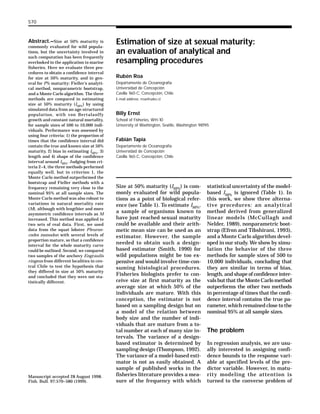
6. 575
Roa et al.: Estimation of size at sexual maturity
percentiles of l50% (Eqs. 3–11) In bootstrap, for each
sample size and each of the 5000 trials, we obtained
Nboot=5000 bootstrap samples. With the Monte Carlo
method, we resampled parameter estimate values
from unbounded normal distributions with NMC=
5000. For completeness, NFieller=1.
In step 1, the deterministic size structure of the
population was conceived as a mixture of normal
probability distributions, each normal distribution
corresponding to an age class. The proportion of in-
dividuals at each size interval was characterized by
the following expression
p
p
p l
n
n t
t
n t
t
l
l
t
t
=
−
−
−
−
=
=
=
∑
∑
∑
2
1
2
1
2
1
2
2
2
0
9
2
2
0
9
0
40
πσ
µ
σ
πσ
µ
σ
exp
exp
,
(16)
where the sum is over 10 age classes (0 to 9) and 41
size classes (0 to 40), and where µt is determined by
a growth equation
µ µ
t
k t t
e
= −
( )
∞
− −
1 0
( )
(17)
with known parameters (Table 2). Variance of size-
at-age (σ2) is known and constant through age (Table
2), and the proportion of individuals at age (Pnt) is
given by a simple exponential mortality model
P
e
e
n
Mt
Mt
t
t
=
−
−
=
∑
0
9
,
(18)
where the mortality rate (M) is known and constant
through age (Table 2).
Random variability came from two sources. First,
samples of the specified sizes were drawn, for each
trial, from a uniform probability distribution and
compared with the cumulative distribution of Equa-
tion 16, accumulating the scores in the respective
size intervals. This computation yielded a sample of
relative size frequencies pnl. Next, we introduced the
second source of uncertainty by assessing the matu-
rity status (mature or immature) of individuals be-
longing to each size class. This random assignment
of maturity status came from resampling the bino-
mial probability distribution
P n n
n
n
P l P l
rand
l rand
rand
n n n
rand t rand rand
( ) ( ) ( ) ,
, ( )
,
= =
−
( )
−
1 (19)
where P(l) was computed from the logistic model (Eq.
1) with known maturity parameters (Table 2) and
nrand is the random number of mature individuals
out of nl,rand=Nsample × pnl individuals in the size in-
terval l. In this way, step 1 was completed by ran-
domly assigning two properties to each data indi-
vidual: a size (continuous variable) and a maturity
status (dichotomous variable). With these data, step
2 was completed by using a nonlinear parameteriza-
tion of the logistic model (Eqs. 1 and 2) for obtaining
estimates of β0 and β1, and their covariance matrix,
by means of the SIMPLEX algorithm (Press et al.,
1992). Having this information in hand, step 3 was
completed by obtaining 2.5%, 50%, and 97.5% per-
centiles by each of the three methods. We pro-
grammed the MATSIMVL algorithm using Microsoft
FORTRAN for PowerStation 4.0 (Microsoft Corp.,
1995).
In the case of the Monte Carlo algorithm, we also
investigated the effect of the natural mortality pa-
rameter, by varying its level in simulation at M=0.2,
M=0.4, M=0.6, and M=0.8, for sample sizes of
Nsample=1000 and 5000 individuals. Niter and NMC
were both kept at 5000.
Finally, we introduce real data to show two appli-
cations of the Monte Carlo method developed here.
First, we estimate lP% (NMC=5000) for a single popu-
lation of the galatheid decapod Pleuroncodes
monodon. In this application, we estimate size con-
fidence intervals for percentages of maturity from
10% to 90% at steps of 10%. In this way a confidence
interval for the whole maturity curve is outlined.
Second, we compare samples of female anchovy
Engraulis ringens from two localities 3° of latitude
apart (NMC=5000) to test the null hypothesis of equal
l50% between them.
Results
The simulation analysis with MATSIMVL yielded
size-at-age and maturity-at-size data with the ap-
propriate behavior as Nsample increased: size-fre-
quency distributions became smoother and maturity
data more closely followed a logistic curve, as shown
by one example output of MATSIMVL data-simulat-
ing routines (Fig. 1).
A summary of the simulation results is presented
in Fig. 2. It shows that, under the simulation condi-
tions, the Monte Carlo method outperformed the
bootstrap and the Fieller methods in proportion of
success at all sample sizes and that it remained very
close to the nominal 95%; the bootstrap method suc-
ceeded 94% or less at all sample sizes, whereas the
Fieller method was unstable between sample sizes
of 500 to 5000, with a minimum of 93% success at
3000 (Fig. 2A). All three methods showed negligible
7. 576 Fishery Bulletin 97(3), 1999
Figure 1
Example output of simulated data on size frequency and maturity-at-size generated by one trial of the
MATSIMVL algorithm, for sample sizes of 500 (A and B ), 1000 (C and D), 3000 (E and F), 5000 (G and H),
and 10,000 (I and J) individuals.
bias at low sample sizes and converged neatly to null
bias at large sample sizes (Fig. 2C). Likewise, the
three methods behaved exactly the same in length
of confidence interval, decaying exponentially as
sample size increased (Fig. 2C). Finally, both
resampling methods yielded asymmetrical (right-
tailed) confidence intervals, converging to the same
shape value (ca. 1.1) as sample size increased (by
definition, Fieller’s method yields a symmetrical con-
fidence interval with shape=1).
Percentage success and bias of the Monte Carlo
method under our model for data generation were
fairly insensitive to changes in natural mortality M
(Fig. 3) for sample sizes of 1000 and 5000 individu-
als. Percentage success remained close to the nomi-
nal 95% and bias was negligible. The length of the
confidence interval and asymmetry, however, in-
creased with increasing mortality, showing that es-
timation variance was directly proportional to natu-
ral mortality rate.
Results of the Monte Carlo algorithm with real
data on female squat lobster are shown in Figure 4.
The Monte Carlo confidence interval for l50% was
fairly narrow (25.86 to 28.51 mm carapace length),
8. 577
Roa et al.: Estimation of size at sexual maturity
Figure 2
Summary of results from the application of the three methods to simulated data. Open squares = Fieller’s ana-
lytical method; open circles: bootstrap; closed circles = Monte Carlo.
reflecting the effect of large sample size (Nsample=
4458). The Monte Carlo median l50% (27.19 mm cara-
pace length) coincided with the MLE of l50%=–MLE
(β0)(MLE(β1). The amplitude of the confidence inter-
val for lP% showed an increasing trend towards ex-
treme values of P (Fig. 4), a reflection of the alge-
braic structure of Equation 3. Results of the second
application with two samples of female anchovies are
shown on Figure 5. Although different in their
lengths, probably due to different sample sizes, con-
fidence intervals from the two samples overlapped and
have the same upper limit. This result provides sup-
port to the hypothesis of equal maturity schedules be-
tween female anchovies from the two localities.
Discussion
The logistic model is universally used as a math-
ematical description of the relation between body size
and sexual maturity. To model residuals, however,
two different approaches emerge: to consider them
normally or binomially distributed, and closely re-
lated to this, to use the data as proportions or as
counts. In the first (as far as we know) formal treat-
ment of the problem, Leslie et al. (1945) used the
data as proportions, transformed to probit scores, and
assumed the normal distribution. Current research-
ers have not employed probit transformations (but
see Lovrich and Vinuesa, 1993) but have continued
using data as proportions and the normal distribu-
tion for residuals (Table 1). In this work however,
and following the arguments by Welch and Foucher
(1988), we emphasize the need to estimate the ma-
turity model using the data as counts and therefore
to consider residuals as binomially distributed. Un-
der this approach, the standard procedure for fitting
the maturity model is logistic regression (Hosmer and
Lemeshow, 1989).
When the model has been fitted, the problem of
setting a confidence interval for the level of the pre-
dictor variable (size) that gives rise to a fixed pro-
portion of maturity is not trivial. We have explored
here three approaches: one analytical method based
9. 578 Fishery Bulletin 97(3), 1999
Figure 3
Effect on natural mortality rate on the performance of the Monte Carlo method. Open circles =1000 indi-
viduals; closed circles = 5000 individuals. Nsample= 5000, NMC= 5000.
on Fieller’s (1944) theorem and the logit link func-
tion, and two computationally-intensive methods
based on nonparametric bootstrap of the observa-
tional pair (li,hi) and Monte Carlo resampling of pa-
rameter estimates from the logistic model. Although
this is not an exhaustive set of methods (for example,
we did not explore likelihood profiles), they repre-
sent a set of conceptually different alternatives to be
tested against the model we used to generate simu-
lated data. In particular, both resampling methods
are especially useful to obtain the distribution of a
function of estimated parameters, such as in Equa-
tion 3, mainly because of their mathematical sim-
plicity, which comes at the expense of extensive com-
putation. Our results indicate that the three meth-
ods to estimate size at P% maturity perform almost
equally well in terms of bias, length, and shape of
the confidence interval, but that Monte Carlo per-
formed better in containing the true parameter
within its confidence bounds with the nominal 95%
rate. This greater accuracy is accompanied by Nboot–1
times less computation than bootstrap.
Bootstrap single assumption was that all observa-
tions from any given sample have the same prob-
ability to appear in a new sample. In contrast, the
Monte Carlo method assumed a bivariate normal
distribution of parameter estimates of the maturity
model. Having simpler assumptions, it is unclear why
the bootstrap method failed more than the nominal
5% of the times at low sample sizes. One reasonable
explanation is that for every sample, there would be
Nboot bootstrap samples, and therefore Nboot numeri-
cal solutions to the normal equations under the bi-
nomial likelihood model. We used here 5000 boot-
strap samples and the SIMPLEX algorithm (Press
et al., 1992). Small errors in the numerical algorithm
coupled with a minimum bias, may add to the nomi-
nal 5%, accounting for the 1% to 2% increase in fail-
ure rate. In contrast, the Monte Carlo algorithm re-
quires a single numerical solution so that it does not
accumulate numerical errors. On the other hand,
Fieller’s analytical method requires a more compli-
cated set of assumptions than the Monte Carlo ap-
proach. Fieller’s method requires normality of a lin-
10. 579
Roa et al.: Estimation of size at sexual maturity
Figure 5
Monte Carlo confidence intervals for length at 50% maturity of female
anchovies (Engraulis ringens) sampled from two localities off central Chile.
Open circles and dotted line = Talcahuano (36°45'S) (Nsample=783,
NMC=5000); Closed circles and solid line = San Antonio (33°35'S)
(Nsample=585, NMC=5000); Closed squares = 95% confidence bounds for l50%.
Figure 4
Monte Carlo confidence intervals for P% maturity for female squat lob-
sters, Pleuroncodes monodon (Nsample=4458, NMC=5000). Open circles = raw
data; continuous line = fitted model; closed squares = Monte Carlo confi-
dence bounds for length at P% maturity (P=0.0–1.0 in steps of 0.1).
ear combination of parameter estimates
and therefore assumes a symmetric in-
terval estimate. Both bootstrap and
Monte Carlo results indicate that the
interval estimate can be quite asymmet-
ric. This may account for the better per-
formance of Monte Carlo, as compared
with Fieller’s, in proportion of success.
These remarks, along with the facts
that Monte Carlo’s percentage success
and bias are not affected by a natural
mortality rate varying between 0.2 and
0.8, and that it is very fast on every com-
puter platform, allows us to recommend
the use of the Monte Carlo method to
estimate size at P% maturity.
Acknowledgments
We would like to thank Bryan F. J.
Manly for reviewing an earlier draft of
this work and three anonymous review-
ers who made several comments and
criticisms which greatly improved the
manuscript. This work was funded by
FONDECYT grant 1950090 to R.R.
11. 580 Fishery Bulletin 97(3), 1999
Literature cited
Armstrong, M. P., J. A. Musick, and J. A. Convocoresses.
1992. Age, growth, and reproduction of the goosefish
Lophius americanus (Pisces: Lophiiformes). Fish. Bull.
90:217–230.
Campbell, A., and M. D. Eagles.
1983. Size at maturity and fecundity of rock crabs, Cancer
irroratus, from the Bay of Fundy and southwestern Nova
Scotia. Fish. Bull. 81(2):357–362.
Campbell, A., and D. G. Robinson.
1983. Reproductive potential of three American lobster
(Homarus americanus) stocks in the Canadian maritimes.
Can. J. Fish. Aquat. Sci. 40:1958–1967.
Casella, G., and R. L. Berger.
1990. Statistical inference. Brooks and Cole Publ. Co.,
Duxbury, California. 650 p.
Chambers, J. M.
1977. Computational methods for data analysis. John
Wiley and Sons, New York, NY, 268 p.
Comeau, M., and G. Y. Conan.
1992. Morphometry and gonad maturity of male snow crab,
Chionoecetes opilio. Can. J. Fish. Aquat. Sci., 49:2460–
2468.
Draper, N. R., and H. Smith.
1981. Applied regression analysis. John Wiley and Sons,
New York, NY, 736 p.
Efron, B., and R. J. Tibshirani.
1993. An introduction to the bootstrap. Chapman & Hall,
New York, NY, 436 p.
Fieller, E. C.
1944. A fundamental formula in the statistics of biological
assay, and some applications. Quart. J. Pharm. 17:117–
123.
Finney, D. J.
1977. Probit analysis, 3rd ed. Cambridge Univ. Press, New
York, NY, 333 p.
Gaertner, D., and F. Laloé.
1986. Étude biométrique de la taille à première maturité
sexuelle de Geryon maritae Manning et Holthuis, 1981 du
Sénégal. Oceanol. Acta 9:479–487.
González-Gurriarán, E., and J. Freire.
1994. Sexual maturity in the velvet swimming crab Necora
puber (Brachyura, Portunidae): morphometric and repro-
ductive analyses. ICES J. Mar. Sci., 51:133–145.
Hosmer, D. W., and S. Lemeshow.
1989. Applied logistic regression. John Wiley and Sons,
New York, NY, 328 p.
Johansen, S.
1984. Functional relations, random coefficients, and non-
linear regression with application to kinetic data.
Springer-Verlag, New York, NY, 126 p.
Leslie, P. H., J. S. Perry, and J. S. Watson.
1945. The determination of the median body-weight at
which female rats reach maturity. Proc. Zool. Soc. Lond.
115:473–488.
Lovrich, G. A., and J. H. Vinuesa.
1993. Reproductive biology of the false southern king crab
(Paralomis granulosa, Lithodidae) in the Beagle Channel,
Argentina. Fish. Bull. 91:664–675.
Manly, B. F. J.
1997. Randomization, bootstrap and Monte Carlo methods
in biology, 2nd ed. Chapman & Hall, London, 399 p.
Microsoft Corp.
1995. FORTRAN PowerStation programmer’s guide.
Printed in the USA, 752 p.
McCullagh, P., and J. A. Nelder.
1989. Generalized linear models. Chapman & Hall, Lon-
don. 511 p.
Press, W. H., S. A. Teukolsky, W. T. Vettering, and
B. P. Flannery.
1992. Numerical recipes in FORTRAN, 2nd ed. Cambridge
Univ. Press, Cambridge, 963 p.
Roa, R.
1993a. Annual growth and maturity function of the squat
lobster Pleuroncodes monodon in central Chile. Mar. Ecol.
Prog. Ser. 97:157–166.
1993b. Análisis metodológico pesquería de langostino
colorado. Tech. Rep., Instituto de Fomento Pesquero
(IFOP), Chile. 86 p. [Available from Subsecretaría de Pesca,
Bellavista 168, piso 19, Valparaíso, Chile.]
Shanubhogue, A., and P. A. Gore.
1987. Using logistic regression in ecology. Curr. Sci. 56:
933–936.
Smith, S. J.
1990. Use of statistical models for the estimation of abun-
dance from groundfish trawl survey data. Can. J. Fish.
Aquat. Sci. 47:894–903.
Somerton, D. A.
1980. A computer technique for estimating the size of sexual
maturity in crabs. Can. J. Fish. Aquat. Sci., 37:1488–
1494.
Somerton, D. A., and R. A. MacIntosh.
1983. The size at sexual maturity of blue king crab,
Paralithodes platypus, in Alaska. Fish. Bull. 81(3):621–
628.
Somerton, D. A., and R. S. Otto.
1986. Distribution and reproductive biology of the golden
king crab, Lithodes aequispina, in the eastern Bering
Sea. Fish. Bull. 84(3):571–584.
Thompson, S. K.
1992. Sampling. John Wiley & Sons, New York, NY,
343 p.
Welch, D. W., and R. P. Foucher.
1988. A maximum likelihood methodology for estimating
length-at-maturity with application to Pacific cod (Gadus
macrocephalus) population dynamics. Can. J. Fish.
Aquat. Sci. 45:333–343.