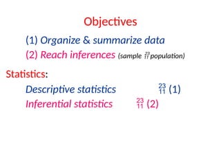
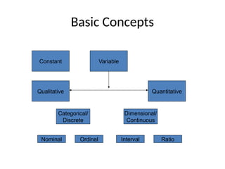
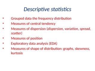
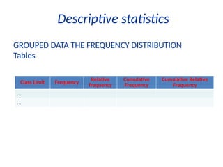
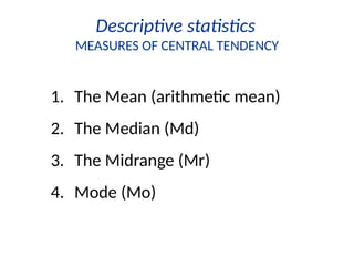
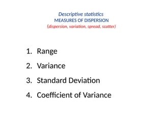
Introduction to Statistics
Basic Concepts
Intro. to Statistics
• What is Statistics?
– “…a set of procedures and rules…for reducing
large masses of data to manageable proportions
and for allowing us to draw conclusions from
those data”
Objectives
(1) Organize & summarize data
(2) Reach inferences (sample  population)
Statistics:
Descriptive statistics  (1)
Inferential statistics  (2)
1.1: What is Statistics?
Two areas of statistics:
Descriptive Statistics: collection, presentation,
and description of sample data.
It is the analysis of data that helps describe,
show or summarize data in a meaningful way
such that, for example, patterns might emerge
from the data.
Basic Concepts
Constant Variable
Qualitative Quantitative
Categorical/
Discrete
Dimensional/
Continuous
Nominal Ordinal Interval Ratio
Inferential Statistics:
It is used to make decisions and draw
conclusions about populations.
we use inferential statistics to try to deduce
from the sample data what the population might
think. Or, we use inferential statistics to make
judgments of the probability that an observed
difference between groups is a dependable one
or one that might have happened by chance in
this study.
Example: A recent study examined the math and verbal SAT
scores of high school seniors across the country. Which of
the following statements are descriptive in nature and
which are inferential.
• The mean math SAT score was 492.
• The mean verbal SAT score was 475.
• Students in the Northeast scored higher in math but lower
in verbal.
• 80% of all students taking the exam were headed for
college.
• 32% of the students scored above 610 on the verbal SAT.
• The math SAT scores are higher than they were 10 years
ago.
1.2 Introduction to Basic Terms
Population: A collection, or set, of individuals or
objects or events whose properties are to be
analyzed.
Two kinds of populations: finite or infinite.
Sample: A subset of the population.
Variable: A characteristic about each individual element of a
population or sample.
Data (singular): The value of the variable associated with one
element of a population or sample. This value may be a
number, a word, or a symbol.
Data (plural): The set of values collected for the variable from
each of the elements belonging to the sample.
Experiment: A planned activity whose results yield a set of
data.
Parameter: A numerical value summarizing all the data of an
entire population.
Statistic: A numerical value summarizing the sample data.
Example: A college dean is interested in learning about the average age
of faculty. Identify the basic terms in this situation.
The population is the age of all faculty members at the college.
A sample is any subset of that population. For example, we might select
10 faculty members and determine their age.
The variable is the “age” of each faculty member.
One data would be the age of a specific faculty member.
The data would be the set of values in the sample.
The experiment would be the method used to select the ages forming the
sample and determining the actual age of each faculty member in the
sample.
The parameter of interest is the “average” age of all faculty at the
college.
The statistic is the “average” age for all faculty in the sample.
Basic Terminology
• Most often, the aim of our research is not to
infer characteristics of a population from our
sample, but to compare two samples
– I.e. To determine if a particular treatment works,
we compare two groups or samples, one with the
treatment and one without
Basic Terminology
– We draw conclusions based on how similar the two groups
are
• If the treated and untreated groups are very similar, we cannot
declare the treatment much of a success
• Another way of putting this in terms of samples and
populations is determining if our two groups/samples
actually come from the same population, or two
different ones
Basic Terminology
• Group A (Treated) and B (Untreated) are
sampled from different populations/treatment
worked:
Group A
Population of Healthy People
Group B
Population of Sick People
Basic Terminology
• Group A and B are sampled from the same
population/treatment didn’t work:
Group A
Group B
Population of Sick People
Basic Terminology
• What if Group A (who received the Tx) were
sicker then Group B (who did not receive Tx),
prior to treatment? What would their scores
look like after Tx?
– The inability to attribute changes in the variable of
interest to the manipulation – poor internal
validity
• I.e. we can’t say for sure if our experiment worked or
not
Basic Terminology
• Quantitative Data
– Dimensional/Measurement Data versus
Categorical/Frequency Count Data
• Dimensional
– When quantities of something are measured on a continuum
– Answers “how much” questions
– I.e. scores on a test, measures of weight, etc.
Basic Terminology
• Categorical
– When numbers of discrete entities have to be counted
» Gender is an example of a discrete entity – you can be
either male or female, and nothing else – speaking of
“degree of maleness” makes little sense
– Answers “how many” questions
– I.e. number of men and women, percentage of people with a
given hair color
Basic Terminology
• A dimensional variable can be converted into
a categorical one
– Convert scores on a test (0-100) into “Low”,
“Medium”, and “High” groups – 0-33 = Low; 34-66
= Medium, and 67-100 = High
• The groups are discrete categories (hence
“categorical”), and you would now count how many
people fall into each category
Two kinds of variables:
Qualitative, or Attribute, or Categorical, Variable: A
variable that categorizes or describes an element of
a population.
Note: Arithmetic operations, such as addition and
averaging, are not meaningful for data resulting from
a qualitative variable.
Quantitative, or Numerical, Variable: A variable that
quantifies an element of a population.
Note: Arithmetic operations such as addition and
averaging, are meaningful for data resulting from a
quantitative variable.
Examples
• Qualitative Distinctions:
– “Good” versus “Bad”
– “Right” versus “Wrong”
– “A Lot” versus “A Little”
• Quantitative Distinctions:
– 5 1/7 versus 4 ¼
– 25% versus 50%
– 1 hour versus 24 hours
Quantative vs. Qualitative
• “Quantitative”
– Involves measurement
– Data in numerical form
– Answers “How much” questions
– Objective and results in unambiguous conclusions
• “Qualitative”
– Describes the nature of something
– Answers “What” or “Of what kind” questions
– Often evaluative and ambiguous
Example: Identify each of the following examples as attribute (qualitative) or
numerical (quantitative) variables.
1. The residence hall for each student in a statistics class.
2. (Attribute)
2. The amount of gasoline pumped by the next 10 customers at the local
Unimart.
(Numerical)
3. The amount of radon in the basement of each of 25 homes in a new
development.
(Numerical)
4. The color of the baseball cap worn by each of 20 students.
(Attribute)
5. The length of time to complete a mathematics homework assignment.
(Numerical)
6. The state in which each truck is registered when stopped and inspected at a
weigh station.
(Attribute)
Qualitative and quantitative variables may be further
subdivided:
Nominal
Qualitative
Ordinal
Variable
Discrete
Quantitative
Continuous
Nominal Variable: A qualitative variable that categorizes (or
describes, or names) an element of a population.
Ordinal Variable: A qualitative variable that incorporates an
ordered position, or ranking.
Discrete Variable: A quantitative variable that can assume a
countable number of values. Intuitively, a discrete variable
can assume values corresponding to isolated points along a
line interval. That is, there is a gap between any two values.
Continuous Variable: A quantitative variable that can assume
an uncountable number of values. Intuitively, a continuous
variable can assume any value along a line interval, including
every possible value between any two values.
Note:
1. In many cases, a discrete and continuous variable may
be distinguished by determining whether the variables
are related to a count or a measurement.
2. Discrete variables are usually associated with counting.
If the variable cannot be further subdivided, it is a clue
that you are probably dealing with a discrete variable.
3. Continuous variables are usually associated with
measurements. The values of discrete variables are
only limited by your ability to measure them.
Example: Identify each of the following as examples of
qualitative or numerical variables:
1. The temperature in Barrow, Alaska at 12:00 pm on
any
given day.
2. The make of automobile driven by each faculty
member.
3. Whether or not a 6 volt lantern battery is defective.
4. The weight of a lead pencil.
5. The length of time billed for a long distance
telephone call.
6. The brand of cereal children eat for breakfast.
7. The type of book taken out of the library by an adult.
Example: Identify each of the following as examples of (1)
nominal, (2) ordinal, (3) discrete, or (4) continuous variables:
1. The length of time until a pain reliever begins to
work.
2. The number of chocolate chips in a cookie.
3. The number of colors used in a statistics textbook.
4. The brand of refrigerator in a home.
5. The overall satisfaction rating of a new car.
6. The number of files on a computer’s hard disk.
7. The pH level of the water in a swimming pool.
8. The number of staples in a stapler.
Descriptive statistics
• Grouped data the frequency distribution
• Measures of central tendency
• Measures of dispersion (dispersion, variation, spread,
scatter)
• Measures of position
• Exploratory data analysis (EDA)
• Measures of shape of distribution: graphs, skewness,
kurtosis
Descriptive statistics
Class Limit Frequency
Relative
frequency
Cumulative
Frequency
Cumulative Relative
Frequency
...
...
GROUPED DATA THE FREQUENCY DISTRIBUTION
Tables
Descriptive statistics
MEASURES OF CENTRAL TENDENCY
1. The Mean (arithmetic mean)
2. The Median (Md)
3. The Midrange (Mr)
4. Mode (Mo)
Descriptive statistics
MEASURES OF CENTRAL TENDENCY
1. The Mean (arithmetic mean)
2. The Median (Md)
3. The Midrange (Mr)
4. Mode (Mo)
Descriptive statistics
MEASURES OF DISPERSION
(dispersion, variation, spread, scatter)
1. Range
2. Variance
3. Standard Deviation
4. Coefficient of Variance
1.3: Measure and Variability
 No matter what the response variable: there will always be
variability in the data.
 One of the primary objectives of statistics: measuring and
characterizing variability.
 Controlling (or reducing) variability in a manufacturing
process: statistical process control.
Example:A supplier fills cans of soda marked 12 ounces. How much
soda does each can really contain?
 It is very unlikely any one can contains exactly 12 ounces of soda.
 There is variability in any process.
 Some cans contain a little more than 12 ounces, and some cans
contain a little less.
 On the average, there are 12 ounces in each can.
 The supplier hopes there is little variability in the process, that
most cans contain close to 12 ounces of soda.
1.4: Data Collection
 First problem a statistician faces: how to obtain the data.
 It is important to obtain good, or representative, data.
 Inferences are made based on statistics obtained from the
data.
 Inferences can only be as good as the data.
Biased Sampling Method:A sampling method that produces data
which systematically differs from the sampled population. An
unbiased sampling method is one that is not biased.
Sampling methods that often result in biased samples:
1. Convenience sample: sample selected from elements of a
population that are easily accessible.
2. Volunteer sample: sample collected from those elements
of the population which chose to contribute the needed
information on their own initiative.
Process of data collection:
1. Define the objectives of the survey or experiment.
Example: Estimate the average life of an electronic component.
2. Define the variable and population of interest.
Example: Length of time for anesthesia to wear off after surgery.
3. Defining the data-collection and data-measuring schemes. This
includes sampling procedures, sample size, and the data-measuring
device (questionnaire, scale, ruler, etc.).
4. Determine the appropriate descriptive or inferential data-analysis
techniques.
Methods used to collect data:
Experiment:The investigator controls or modifies the environment
and observes the effect on the variable under study.
Survey: Data are obtained by sampling some of the population of
interest. The investigator does not modify the environment.
Census:A 100% survey. Every element of the population is listed.
Seldom used: difficult and time-consuming to compile, and
expensive.
shafiqurrehman1@yahoo.com
Sampling Frame:A list of the elements belonging to the
population from which the sample will be drawn.
Note: It is important that the sampling frame be representative of the
population.
Sample Design:The process of selecting sample elements from the
sampling frame.
Note:There are many different types of sample designs. Usually they
all fit into two categories: judgment samples and probability samples.
Judgment Samples: Samples that are selected on the basis of being
“typical.”
Items are selected that are representative of the population. The
validity of the results from a judgment sample reflects the soundness
of the collector’s judgment.
Probability Samples: Samples in which the elements to be
selected are drawn on the basis of probability. Each element in a
population has a certain probability of being selected as part of the
sample.
Random Samples:A sample selected in such a way that every
element in the population has a equal probability of being chosen.
Equivalently, all samples of size n have an equal chance of being
selected. Random samples are obtained either by sampling with
replacement from a finite population or by sampling without
replacement from an infinite population.
Note:
1. Inherent in the concept of randomness: the next result (or occurrence) is not predictable.
2. Proper procedure for selecting a random sample: use a random number generator or a
table of random numbers.
Example:An employer is interested in the time it takes each employee
to commute to work each morning. A random sample of 35
employees will be selected and their commuting time will be
recorded.
There are 2712 employees.
Each employee is numbered: 0001, 0002, 0003, etc. up to 2712.
Using four-digit random numbers, a sample is identified: 1315,
0987, 1125, etc.
Systematic Sample:A sample in which every kth item of the
sampling frame is selected, starting from the first element which is
randomly selected from the first k elements.
Note:The systematic technique is easy to execute. However, it has
some inherent dangers when the sampling frame is repetitive or
cyclical in nature. In these situations the results may not
approximate a simple random sample.
Stratified Random Sample:A sample obtained by stratifying the
sampling frame and then selecting a fixed number of items from each
of the strata by means of a simple random sampling technique.
Descriptive statistics
MEASURES OF SHAPE OF DISTRIBUTION
Graphs
• Frequency distribution
• Relative frequency of occurrence
 proportion of values
Nominal, Ordinal level
• Bar chart
• Pie chart
Interval, Ratio level
• The histogram: frequency
histogram & relative frequency
histogram
• Frequency polygon: midpoint
of class interval
• Pareto chart: bar chart with
descending sorted frequency
• Cumulative frequency
• Cumulative relative frequency
→ OGIVE graph (Ojiv or Oh’-
jive graph)
Descriptive statistics
MEASURES OF SHAPE OF DISTRIBUTION
Skewness, Kurtosis
• Skewness (Sk), Pearsonian coefficient, is a measure of
asymmetry of a distribution around its mean.
• Kurtosis characterizes the relative peakedness or
flatness of a distribution compared with the normal
distribution.
Inferential statistics
Hypothesis testing
 reaching a decision
Inferential statistics
Estimation
• Estimation (or estimating) is the process of
finding an estimate, or approximation, which is
a value that is usable for some purpose even if
input data may be incomplete, uncertain, or
unstable.
• a rough calculation of the value, number,
quantity, or extent of something.
• a judgment of the worth or character of
someone or something.
Inferential statistics
drawing of inferences
- Estimation
- Hypothesis testing  reaching a decision
+ Parametric statistics
+ Non-parametric statistics << Distribution-free statistics
- Modeling, Predicting
What statistical calculations cannot do
• Choosing good sample
• Choosing good variables
• Measuring variables precisely
Design Data summary Statistics & Tests
2 independent groups Proportions
Rank Ordered
Mean
Survival
Chi-square, Fisher-exact
Mann-Whitney U
Unpaired t-test
Mantel-Haenzel, Log rank
2 related groups Proportions
Rank Ordered
Mean
McNemar Chi-square
Sign test
Wilcoxon signed rank
Paired t-test
More than 2 independent
groups
Proportions
Rank Ordered
Mean
Survival
Chi-square
Kruskal-Wallis
ANOVA
Log rank
More than 2 related groups Proportions
Rank Ordered
Mean
Cochran Q
Friedman
Repeated ANOVA
Study of Causation; one
independent variable
(univariate)
Proportion
Mean
Relative Risk
Odd Ratios
Correlation coefficient
Study of Causation; more
than one independent
variable (Multivariate)
Proportion
Mean
Discriminant Analysis
Multiple Logistic Regression
Log Linear Model
Regression Analysis
Multiple Classification Analysis

1-Introduction to Statistics ppt xv.pptx

  • 1.
  • 2.
    Intro. to Statistics •What is Statistics? – “…a set of procedures and rules…for reducing large masses of data to manageable proportions and for allowing us to draw conclusions from those data”
  • 3.
    Objectives (1) Organize &summarize data (2) Reach inferences (sample  population) Statistics: Descriptive statistics  (1) Inferential statistics  (2)
  • 4.
    1.1: What isStatistics? Two areas of statistics: Descriptive Statistics: collection, presentation, and description of sample data. It is the analysis of data that helps describe, show or summarize data in a meaningful way such that, for example, patterns might emerge from the data.
  • 5.
    Basic Concepts Constant Variable QualitativeQuantitative Categorical/ Discrete Dimensional/ Continuous Nominal Ordinal Interval Ratio
  • 6.
    Inferential Statistics: It isused to make decisions and draw conclusions about populations. we use inferential statistics to try to deduce from the sample data what the population might think. Or, we use inferential statistics to make judgments of the probability that an observed difference between groups is a dependable one or one that might have happened by chance in this study.
  • 7.
    Example: A recentstudy examined the math and verbal SAT scores of high school seniors across the country. Which of the following statements are descriptive in nature and which are inferential. • The mean math SAT score was 492. • The mean verbal SAT score was 475. • Students in the Northeast scored higher in math but lower in verbal. • 80% of all students taking the exam were headed for college. • 32% of the students scored above 610 on the verbal SAT. • The math SAT scores are higher than they were 10 years ago.
  • 8.
    1.2 Introduction toBasic Terms Population: A collection, or set, of individuals or objects or events whose properties are to be analyzed. Two kinds of populations: finite or infinite. Sample: A subset of the population.
  • 9.
    Variable: A characteristicabout each individual element of a population or sample. Data (singular): The value of the variable associated with one element of a population or sample. This value may be a number, a word, or a symbol. Data (plural): The set of values collected for the variable from each of the elements belonging to the sample. Experiment: A planned activity whose results yield a set of data. Parameter: A numerical value summarizing all the data of an entire population. Statistic: A numerical value summarizing the sample data.
  • 10.
    Example: A collegedean is interested in learning about the average age of faculty. Identify the basic terms in this situation. The population is the age of all faculty members at the college. A sample is any subset of that population. For example, we might select 10 faculty members and determine their age. The variable is the “age” of each faculty member. One data would be the age of a specific faculty member. The data would be the set of values in the sample. The experiment would be the method used to select the ages forming the sample and determining the actual age of each faculty member in the sample. The parameter of interest is the “average” age of all faculty at the college. The statistic is the “average” age for all faculty in the sample.
  • 11.
    Basic Terminology • Mostoften, the aim of our research is not to infer characteristics of a population from our sample, but to compare two samples – I.e. To determine if a particular treatment works, we compare two groups or samples, one with the treatment and one without
  • 12.
    Basic Terminology – Wedraw conclusions based on how similar the two groups are • If the treated and untreated groups are very similar, we cannot declare the treatment much of a success • Another way of putting this in terms of samples and populations is determining if our two groups/samples actually come from the same population, or two different ones
  • 13.
    Basic Terminology • GroupA (Treated) and B (Untreated) are sampled from different populations/treatment worked: Group A Population of Healthy People Group B Population of Sick People
  • 14.
    Basic Terminology • GroupA and B are sampled from the same population/treatment didn’t work: Group A Group B Population of Sick People
  • 15.
    Basic Terminology • Whatif Group A (who received the Tx) were sicker then Group B (who did not receive Tx), prior to treatment? What would their scores look like after Tx? – The inability to attribute changes in the variable of interest to the manipulation – poor internal validity • I.e. we can’t say for sure if our experiment worked or not
  • 16.
    Basic Terminology • QuantitativeData – Dimensional/Measurement Data versus Categorical/Frequency Count Data • Dimensional – When quantities of something are measured on a continuum – Answers “how much” questions – I.e. scores on a test, measures of weight, etc.
  • 17.
    Basic Terminology • Categorical –When numbers of discrete entities have to be counted » Gender is an example of a discrete entity – you can be either male or female, and nothing else – speaking of “degree of maleness” makes little sense – Answers “how many” questions – I.e. number of men and women, percentage of people with a given hair color
  • 18.
    Basic Terminology • Adimensional variable can be converted into a categorical one – Convert scores on a test (0-100) into “Low”, “Medium”, and “High” groups – 0-33 = Low; 34-66 = Medium, and 67-100 = High • The groups are discrete categories (hence “categorical”), and you would now count how many people fall into each category
  • 19.
    Two kinds ofvariables: Qualitative, or Attribute, or Categorical, Variable: A variable that categorizes or describes an element of a population. Note: Arithmetic operations, such as addition and averaging, are not meaningful for data resulting from a qualitative variable. Quantitative, or Numerical, Variable: A variable that quantifies an element of a population. Note: Arithmetic operations such as addition and averaging, are meaningful for data resulting from a quantitative variable.
  • 20.
    Examples • Qualitative Distinctions: –“Good” versus “Bad” – “Right” versus “Wrong” – “A Lot” versus “A Little” • Quantitative Distinctions: – 5 1/7 versus 4 ¼ – 25% versus 50% – 1 hour versus 24 hours
  • 21.
    Quantative vs. Qualitative •“Quantitative” – Involves measurement – Data in numerical form – Answers “How much” questions – Objective and results in unambiguous conclusions • “Qualitative” – Describes the nature of something – Answers “What” or “Of what kind” questions – Often evaluative and ambiguous
  • 22.
    Example: Identify eachof the following examples as attribute (qualitative) or numerical (quantitative) variables. 1. The residence hall for each student in a statistics class. 2. (Attribute) 2. The amount of gasoline pumped by the next 10 customers at the local Unimart. (Numerical) 3. The amount of radon in the basement of each of 25 homes in a new development. (Numerical) 4. The color of the baseball cap worn by each of 20 students. (Attribute) 5. The length of time to complete a mathematics homework assignment. (Numerical) 6. The state in which each truck is registered when stopped and inspected at a weigh station. (Attribute)
  • 23.
    Qualitative and quantitativevariables may be further subdivided: Nominal Qualitative Ordinal Variable Discrete Quantitative Continuous
  • 24.
    Nominal Variable: Aqualitative variable that categorizes (or describes, or names) an element of a population. Ordinal Variable: A qualitative variable that incorporates an ordered position, or ranking. Discrete Variable: A quantitative variable that can assume a countable number of values. Intuitively, a discrete variable can assume values corresponding to isolated points along a line interval. That is, there is a gap between any two values. Continuous Variable: A quantitative variable that can assume an uncountable number of values. Intuitively, a continuous variable can assume any value along a line interval, including every possible value between any two values.
  • 25.
    Note: 1. In manycases, a discrete and continuous variable may be distinguished by determining whether the variables are related to a count or a measurement. 2. Discrete variables are usually associated with counting. If the variable cannot be further subdivided, it is a clue that you are probably dealing with a discrete variable. 3. Continuous variables are usually associated with measurements. The values of discrete variables are only limited by your ability to measure them.
  • 26.
    Example: Identify eachof the following as examples of qualitative or numerical variables: 1. The temperature in Barrow, Alaska at 12:00 pm on any given day. 2. The make of automobile driven by each faculty member. 3. Whether or not a 6 volt lantern battery is defective. 4. The weight of a lead pencil. 5. The length of time billed for a long distance telephone call. 6. The brand of cereal children eat for breakfast. 7. The type of book taken out of the library by an adult.
  • 27.
    Example: Identify eachof the following as examples of (1) nominal, (2) ordinal, (3) discrete, or (4) continuous variables: 1. The length of time until a pain reliever begins to work. 2. The number of chocolate chips in a cookie. 3. The number of colors used in a statistics textbook. 4. The brand of refrigerator in a home. 5. The overall satisfaction rating of a new car. 6. The number of files on a computer’s hard disk. 7. The pH level of the water in a swimming pool. 8. The number of staples in a stapler.
  • 28.
    Descriptive statistics • Groupeddata the frequency distribution • Measures of central tendency • Measures of dispersion (dispersion, variation, spread, scatter) • Measures of position • Exploratory data analysis (EDA) • Measures of shape of distribution: graphs, skewness, kurtosis
  • 29.
    Descriptive statistics Class LimitFrequency Relative frequency Cumulative Frequency Cumulative Relative Frequency ... ... GROUPED DATA THE FREQUENCY DISTRIBUTION Tables
  • 30.
    Descriptive statistics MEASURES OFCENTRAL TENDENCY 1. The Mean (arithmetic mean) 2. The Median (Md) 3. The Midrange (Mr) 4. Mode (Mo)
  • 31.
    Descriptive statistics MEASURES OFCENTRAL TENDENCY 1. The Mean (arithmetic mean) 2. The Median (Md) 3. The Midrange (Mr) 4. Mode (Mo)
  • 32.
    Descriptive statistics MEASURES OFDISPERSION (dispersion, variation, spread, scatter) 1. Range 2. Variance 3. Standard Deviation 4. Coefficient of Variance
  • 33.
    1.3: Measure andVariability  No matter what the response variable: there will always be variability in the data.  One of the primary objectives of statistics: measuring and characterizing variability.  Controlling (or reducing) variability in a manufacturing process: statistical process control.
  • 34.
    Example:A supplier fillscans of soda marked 12 ounces. How much soda does each can really contain?  It is very unlikely any one can contains exactly 12 ounces of soda.  There is variability in any process.  Some cans contain a little more than 12 ounces, and some cans contain a little less.  On the average, there are 12 ounces in each can.  The supplier hopes there is little variability in the process, that most cans contain close to 12 ounces of soda.
  • 35.
    1.4: Data Collection First problem a statistician faces: how to obtain the data.  It is important to obtain good, or representative, data.  Inferences are made based on statistics obtained from the data.  Inferences can only be as good as the data.
  • 36.
    Biased Sampling Method:Asampling method that produces data which systematically differs from the sampled population. An unbiased sampling method is one that is not biased. Sampling methods that often result in biased samples: 1. Convenience sample: sample selected from elements of a population that are easily accessible. 2. Volunteer sample: sample collected from those elements of the population which chose to contribute the needed information on their own initiative.
  • 37.
    Process of datacollection: 1. Define the objectives of the survey or experiment. Example: Estimate the average life of an electronic component. 2. Define the variable and population of interest. Example: Length of time for anesthesia to wear off after surgery. 3. Defining the data-collection and data-measuring schemes. This includes sampling procedures, sample size, and the data-measuring device (questionnaire, scale, ruler, etc.). 4. Determine the appropriate descriptive or inferential data-analysis techniques.
  • 38.
    Methods used tocollect data: Experiment:The investigator controls or modifies the environment and observes the effect on the variable under study. Survey: Data are obtained by sampling some of the population of interest. The investigator does not modify the environment. Census:A 100% survey. Every element of the population is listed. Seldom used: difficult and time-consuming to compile, and expensive. shafiqurrehman1@yahoo.com
  • 39.
    Sampling Frame:A listof the elements belonging to the population from which the sample will be drawn. Note: It is important that the sampling frame be representative of the population. Sample Design:The process of selecting sample elements from the sampling frame. Note:There are many different types of sample designs. Usually they all fit into two categories: judgment samples and probability samples.
  • 40.
    Judgment Samples: Samplesthat are selected on the basis of being “typical.” Items are selected that are representative of the population. The validity of the results from a judgment sample reflects the soundness of the collector’s judgment. Probability Samples: Samples in which the elements to be selected are drawn on the basis of probability. Each element in a population has a certain probability of being selected as part of the sample.
  • 41.
    Random Samples:A sampleselected in such a way that every element in the population has a equal probability of being chosen. Equivalently, all samples of size n have an equal chance of being selected. Random samples are obtained either by sampling with replacement from a finite population or by sampling without replacement from an infinite population. Note: 1. Inherent in the concept of randomness: the next result (or occurrence) is not predictable. 2. Proper procedure for selecting a random sample: use a random number generator or a table of random numbers.
  • 42.
    Example:An employer isinterested in the time it takes each employee to commute to work each morning. A random sample of 35 employees will be selected and their commuting time will be recorded. There are 2712 employees. Each employee is numbered: 0001, 0002, 0003, etc. up to 2712. Using four-digit random numbers, a sample is identified: 1315, 0987, 1125, etc.
  • 43.
    Systematic Sample:A samplein which every kth item of the sampling frame is selected, starting from the first element which is randomly selected from the first k elements. Note:The systematic technique is easy to execute. However, it has some inherent dangers when the sampling frame is repetitive or cyclical in nature. In these situations the results may not approximate a simple random sample. Stratified Random Sample:A sample obtained by stratifying the sampling frame and then selecting a fixed number of items from each of the strata by means of a simple random sampling technique.
  • 44.
    Descriptive statistics MEASURES OFSHAPE OF DISTRIBUTION Graphs • Frequency distribution • Relative frequency of occurrence  proportion of values Nominal, Ordinal level • Bar chart • Pie chart Interval, Ratio level • The histogram: frequency histogram & relative frequency histogram • Frequency polygon: midpoint of class interval • Pareto chart: bar chart with descending sorted frequency • Cumulative frequency • Cumulative relative frequency → OGIVE graph (Ojiv or Oh’- jive graph)
  • 45.
    Descriptive statistics MEASURES OFSHAPE OF DISTRIBUTION Skewness, Kurtosis • Skewness (Sk), Pearsonian coefficient, is a measure of asymmetry of a distribution around its mean. • Kurtosis characterizes the relative peakedness or flatness of a distribution compared with the normal distribution.
  • 46.
  • 47.
    Inferential statistics Estimation • Estimation(or estimating) is the process of finding an estimate, or approximation, which is a value that is usable for some purpose even if input data may be incomplete, uncertain, or unstable. • a rough calculation of the value, number, quantity, or extent of something. • a judgment of the worth or character of someone or something.
  • 48.
    Inferential statistics drawing ofinferences - Estimation - Hypothesis testing  reaching a decision + Parametric statistics + Non-parametric statistics << Distribution-free statistics - Modeling, Predicting
  • 49.
    What statistical calculationscannot do • Choosing good sample • Choosing good variables • Measuring variables precisely
  • 50.
    Design Data summaryStatistics & Tests 2 independent groups Proportions Rank Ordered Mean Survival Chi-square, Fisher-exact Mann-Whitney U Unpaired t-test Mantel-Haenzel, Log rank 2 related groups Proportions Rank Ordered Mean McNemar Chi-square Sign test Wilcoxon signed rank Paired t-test More than 2 independent groups Proportions Rank Ordered Mean Survival Chi-square Kruskal-Wallis ANOVA Log rank More than 2 related groups Proportions Rank Ordered Mean Cochran Q Friedman Repeated ANOVA Study of Causation; one independent variable (univariate) Proportion Mean Relative Risk Odd Ratios Correlation coefficient Study of Causation; more than one independent variable (Multivariate) Proportion Mean Discriminant Analysis Multiple Logistic Regression Log Linear Model Regression Analysis Multiple Classification Analysis