Download as PDF, PPTX


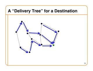
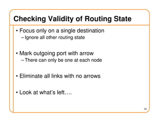
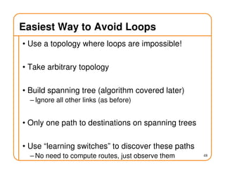
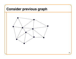
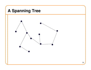
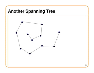
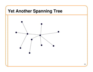
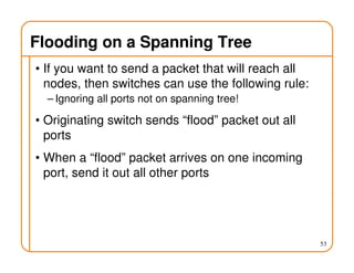
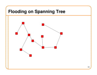
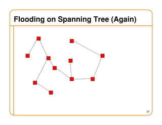
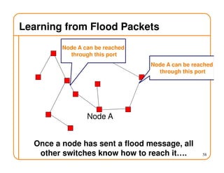
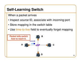
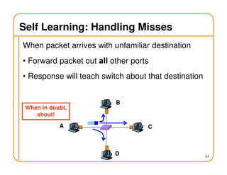
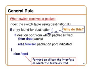


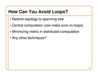


This document provides an overview of routing fundamentals, including: - Routing involves delivering packets from any source to any destination by making forwarding decisions at switches/routers based on routing state. - Routing state can be computed in a distributed manner to avoid loops, such as by minimizing a metric or restricting the network topology to a spanning tree. - On a spanning tree, switches can learn routes by observing packet floods without explicitly computing routes, ensuring there is only one path between any two nodes.