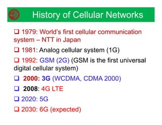
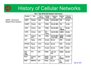
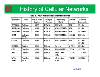
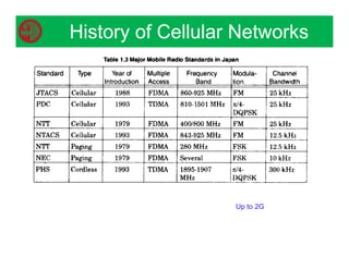
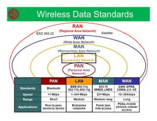
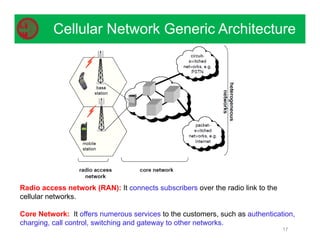
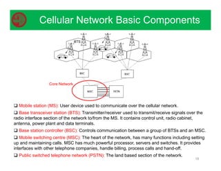
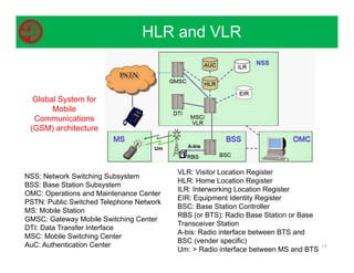
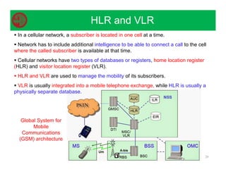
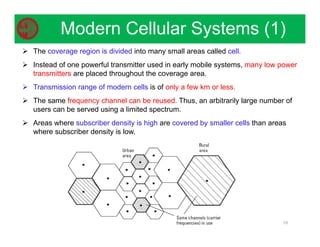
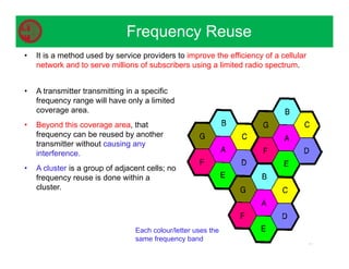
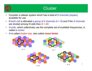
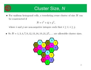
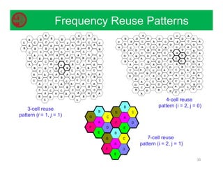
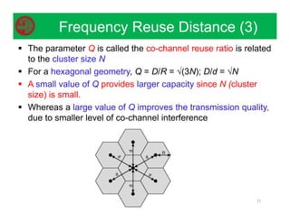
The document discusses various topics related to cellular networks including: - The history of cellular networks from 1G to 5G technologies. - Components of cellular networks including mobile stations, base stations, switches, and databases for tracking user locations. - Concepts like cells, frequency reuse, and handoffs which allow cellular networks to efficiently use limited radio spectrum and maintain connectivity as users move. 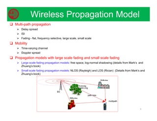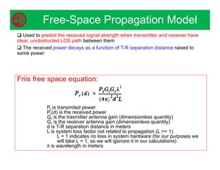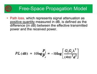- Models for radio propagation including free space path loss which predicts signal strength over distance in line-of-sight conditions. In 3 sentences or less, this summary outlines some of the key technological developments in cellular networks and fundamental concepts that have enabled their widespread adoption and use.

1. 2
Cellular Mobile
Communications

2. Wireless Data Standards
RAN
(Regional Area Network)
IEEE 802.22 Satellite

3. History of Cellular Networks
 1979: World’s first cellular communication
system – NTT in Japan
 1981: Analog cellular system (1G)
 1992: GSM (2G) (GSM is the first universal
digital cellular system)
 2000: 3G (WCDMA, CDMA 2000)
 2008: 4G LTE
 2020: 5G
 2030: 6G (expected)

4. History of Cellular Networks
AMPS - Advanced
Mobile Phone System
Up to 2G

5. History of Cellular Networks
Up to 2G

6. History of Cellular Networks
Up to 2G

7. 8
Wireless Propagation Model
 Multi-path propagation
 Delay spread
 ISI
 Fading - flat, frequency selective, large scale, small scale
 Mobility
 Time-varying channel
 Doppler spread
 Propagation models with large scale fading and small scale fading
 Large scale fading propagation models: free space, log-normal shadowing (details from Mark’s and
Zhuang’s book)
 Small scale fading propagation models: NLOS (Rayleigh) and LOS (Rician) (Details from Mark’s and
Zhuang’s book)

8.  One very powerful transmitter located at the highest spot in an area
 Designed by selecting one or more radio channels for use in a
geographical zone
 A user moving from one zone to another must reinitiate the call
 Hand-off facility is not available
 User capacity is low as it is limited to the number of channels
 High blocking when number of users increases
 Does not use the spectrum efficiently
9
Early Mobile System

9. 10
Modern Cellular Systems (1)
 The coverage region is divided into many small areas called cell.
 Instead of one powerful transmitter used in early mobile systems, many low power
transmitters are placed throughout the coverage area.
 Transmission range of modern cells is of only a few km or less.
 The same frequency channel can be reused. Thus, an arbitrarily large number of
users can be served using a limited spectrum.
 Areas where subscriber density is high are covered by smaller cells than areas
where subscriber density is low.

10.  Frequency reuse provides a much larger number of
communication channels than the number of channels allocated
to the system.
 Automatic inter-cellular transfer, or a handover, ensures
continuity of communication when there is a need to change
BSs.
 Continuous monitoring of communication between the mobile
and BS verifies the quality and detects the need for a cell
transfer.
 Automatic location of mobile stations within the network ensures
that calls can be routed to mobiles.
 Mobile stations continuously listen to a common channel of the
network in order to receive a call.
11
Modern Cellular Systems (2)

11. 12
Modern Cellular Systems (3)
Cells Different
Frequencies or
Codes
Base Station Fixed
transceiver
Mobile Station Distributed
transceivers
Downlink
Uplink
Handoff
Multiple Access

12.  Mobility Management: Users moves from one area to another.
So it is needed.
a. Hand-off management
 When a mobile moves in a different cell while a call in process, the call has
to be transfer from the existing cell to new cell.
 Call must transfer to a new channel of the new cell.
 Done by MSC
b. Location management
 It ensures call routing to the called mobile.
 Must have record in home register about the location of a mobile
 There is a association between home and foreign agents
 Frequency Management
 Channels must be allocated in an efficient manner.
 Interference Management
 Power control and proper RF planning is necessary to manage interference 13
Management Aspects

13. Concept of Cell
14
Antenna
Radiation pattern
'L
UHFW
L
RQDO
$QW
HQQD
What is a cell?
 A cell is the basic geographical unit of a cellular system
 The power of the radio signals transmitted by the BS decays as the signals travel
away from it. A minimum amount of signal strength (let us say, η dB) is needed in order
to be detected by the MS. The region over which the signal strength lies above this
threshold value η dB is known as the coverage area of a BS and it must be a circular
region, considering the BS to be isotropic radiator. Such a circle, which gives this actual
radio coverage, is called the foot print of a cell, or a cell.
 Each cell has a base transceiver station (BTS) / base station (BS) with antenna,
which can be either omnidirectional or directional.

14. Cell Shape (1)
15
 By using hexagonal geometry, the fewest number of cells can cover a
geographic region.
 When using hexagons to model a coverage areas, BS transmitters are
depicted as either being in the center of the cell (center-excited cells) or on
the three of the six cell vertices (edge-excited / corner-excited cells).
 Normally omnidirectional antennas are used in center-excited cells and
directional antennas are used in corner-excited cells.

15. Cell Shape (2)
16
 Hexagonal shaped cells shown in diagram are artificial (abstract) and can’t be
generated in the real world.
 However this shape is chosen to simplify planning and design of a cellular
system as hexagons fit together without any overlap or gap in between them.
 Hexagon geometry requires the fewest number of cells for covering a region.
 Another advantage of using hexagons is that it approaches a circular shape, which
is the ideal power coverage area.
 The real cell shape is as shown above and it's shape will keep changing due to
change in landscape.

16. Cellular Network Generic Architecture
17
Radio access network (RAN): It connects subscribers over the radio link to the
cellular networks.
Core Network: It offers numerous services to the customers, such as authentication,
charging, call control, switching and gateway to other networks.

17. Cellular Network Basic Components
18
 Mobile station (MS): User device used to communicate over the cellular network.
 Base transceiver station (BTS): Transmitter/receiver used to transmit/receive signals over the
radio interface section of the network to/from the MS. It contains control unit, radio cabinet,
antenna, power plant and data terminals.
 Base station controller (BSC): Controls communication between a group of BTSs and an MSC.
 Mobile switching centre (MSC): The heart of the network, has many functions including setting
up and maintaining calls. MSC has much powerful processor, servers and switches. It provides
interfaces with other telephone companies, handle billing, process calls and hand-off.
 Public switched telephone network (PSTN): The land based section of the network.
BTS
Core Network

18. 19
HLR and VLR
Global System for
Mobile
Communications
(GSM) architecture
NSS: Network Switching Subsystem
BSS: Base Station Subsystem
OMC: Operations and Maintenance Center
PSTN: Public Switched Telephone Network
MS: Mobile Station
GMSC: Gateway Mobile Switching Center
DTI: Data Transfer Interface
MSC: Mobile Switching Center
AuC: Authentication Center
VLR: Visitor Location Register
HLR: Home Location Register
ILR: Interworking Location Register
EIR: Equipment Identity Register
BSC: Base Station Controller
RBS (or BTS): Radio Base Station or Base
Transceiver Station
A-bis: Radio interface between BTS and
BSC (vender specific)
Um: Radio interface between MS and BTS

19. 20
HLR and VLR
 In a cellular network, a subscriber is located in one cell at a time.
 Network has to include additional intelligence to be able to connect a call to the cell
where the called subscriber is available at that time.
 Cellular networks have two types of databases or registers, home location register
(HLR) and visitor location register (VLR).
 HLR and VLR are used to manage the mobility of its subscribers.
 VLR is usually integrated into a mobile telephone exchange, while HLR is usually a
physically separate database.
Global System for
Mobile
Communications
(GSM) architecture

20.  The HLR is the global central point (reference database)
where information of clients is available wherever they are
located.
 One network operator can have several HLRs.
 When a subscriber activates a mobile connection, different
information is stored in the HLR of the operator.
 The HLR stores their up-to-date subscriber information, such
as the location, activity status, account status, call forwarding
preference, caller identification preference, etc.
 HLR is now replaced by HSS (Home Subscriber Server) in 4G.
21
HLR (Home Location Register)

21.  VLR stores information about every subscriber in its covered area.
 VLR contains more accurate information of where (to which cell or group of
cells) to connect incoming calls directed to a certain subscriber.
 When a new subscriber arrives in an area, a temporary Mobile Station
Roaming Number (MSRN) is assigned by local VLR to each MS in its area.
MSRN is used to identify the serving MSC/VLR of user to forward an incoming
call.
 VLR also informs the arrival and other data of a new subscriber to the
corresponding HLR.
 Thus, a VLR provides a local database (a copy of most of the data stored at
the HLR) for the subscribers wherever they are physically located. This
function eliminates the need for excessive and time-consuming references to
the “home” HLR database. It is, however, temporary data which exists for only
as long as the subscriber is “active” in that particular area covered by the VLR.
 Grameenphone has 2 HLRs (called HSS in 4G) and 15 VLRs (equivalent block
is MME in 4G).
22
VLR (Visitor Location Register)

22. 23
Basic Operating Principle of a Cellular Network (1)
 Mobile station (MS ) is preprogrammed to know the frequencies of the
control channels.
 When MS is switched on, the mobile scans these frequencies and selects
the BS with the strongest common control channel.
 MS transmits its unique identification code over the control channel in order
to inform the VLR.
 VLR determines the address of the subscriber’s home country and the
home network with the identification of the MS.
 MSC/VLR transmits the signaling message toward the home network,
specially to the HLR to inform the location of this specific subscriber in the
area of a certain VLR.
 HLR stores the location information.
 HLR is able to route the calls to the right MSC/VLR.
 If the MS moves, it changes the channel and the location information, and
the network updates its location information stored in the VLR and HLR.

23. 24
Basic Operating Principle of a Cellular Network (2)

24. 25
Location Updating in GSM
 Each network is divided into small location areas (LAs) that contain a group of cells.
 (1): Mobile A is staying in LA 1. MSC/VLR1 has reported this to Mobile A’s HLR.
 (2) – (3): Mobile A moves to LA 2 and identifies a new LA information (LA2). It
reports its arrival to MSC/VLR 2.
 (4): MSC/VLR 2 informs HLRA, and receives Authentication Data for Mobile A.

25. 26
Calling an MS: MS Originating (Outgoing) Call
1) Via the radio path and the BS network, a call request for GSM subscriber B 9212345 is sent from Mobile A to
MSC/VLR A.
2-3) MSC/VLR A collects authentication data from HLR A (if such data has not been collected earlier).
4) MSC/VLR A requests HLR B of the actual location of GSM subscriber B.
5) Gateway MSC checks with HLR B ”Where is the GSM subscriber?”
6) The call is established to the actual MSC/VLR (Visiting MSC) either directly or through the fixed or
international telephone network
7) The request for mobile 9212345 is transmitted over all BTSs in the actual LA of the called GSM subscriber.
Mobile B recognizes its own identity, and ringing is generated.

26. 27
Frequency Reuse
• A transmitter transmitting in a specific
frequency range will have only a limited
coverage area.
• Beyond this coverage area, that
frequency can be reused by another
transmitter without causing any
interference.
• A cluster is a group of adjacent cells; no
frequency reuse is done within a
cluster.
Each colour/letter uses the
same frequency band
• It is a method used by service providers to improve the efficiency of a cellular
network and to serve millions of subscribers using a limited radio spectrum.

27. • Consider a cellular system which has a total of S channels (duplex)
available for use.
• If each cell is allocated a group of k channels (k S) and if the S channels
are divided among N cells then S = kN.
• N cells, which collectively use the complete set of available frequencies, is
called a cluster.
• N is called cluster size, also called reuse factor.
28
Cluster

28. Cluster Size, N
29

29. Frequency Reuse Patterns
30
3-cell reuse
pattern (i = 1, j = 1)
4-cell reuse
pattern (i = 2, j = 0)
7-cell reuse
pattern (i = 2, j = 1)

30.  Capacity of a cellular system is directly proportional to the number of times a
cluster is replicated in a fixed service area.
 A larger cluster size causes the ratio between the cell radius and the distance
between the co-channel cells to decrease, leading to weaker co-channel
interference.
 Conversely, a small cluster size indicates the co-channel cells are located much
closer together.
 From a designer point of view, the smallest possible value of N is desirable in order
to maximize capacity over a given coverage area
 Example problems of capacity calculation from Zhuang’s book
31
M = Number of times a cluster is replicated (i.e., no. of cluster)
k = Number of channels per cell
Network Capacity

31. 32
How to locate a co-channel cell?
To find the nearest co-channel neighbors of a particular cell, one must do the
following:
(a) move i cells along any chain of hexagons
(b) turn 60 degrees counter-clockwise and move j cells
N = 7, i = 2, j = 1 N = 19, i = 3, j = 2

32. 33
Frequency Reuse Distance (1)

33. 34
Frequency Reuse Distance (2)
You can also use the
“law of cosine”.
Equilateral triangle

34.  The parameter Q is called the co-channel reuse ratio is related
to the cluster size N
 For a hexagonal geometry, Q = D/R = √(3N); D/d = √N
 A small value of Q provides larger capacity since N (cluster
size) is small.
 Whereas a large value of Q improves the transmission quality,
due to smaller level of co-channel interference
35
Frequency Reuse Distance (3)

35. Path-Loss
Models

36. Free-Space Propagation Model
 Used to predict the received signal strength when transmitter and receiver have
clear, unobstructed LOS path between them
 The received power decays as a function of T-R separation distance raised to
some power
Friis free space equation:
Pt is transmited power
Pr(d) is the received power
Gt is the trasmitter antenna gain (dimensionless quantity)
Gr is the receiver antenna gain (dimensionless quantity)
d is T-R separation distance in meters
L is system loss factor not related to propagation (L = 1)
L = 1 indicates no loss in system hardware (for our purposes we
will take L = 1, so we will igonore it in our calculations)
λ is wavelength in meters

37. Free-Space Propagation Model
• Path loss, which represents signal attenuation as
positive quantity measured in dB, is defined as the
difference (in dB) between the effective transmitted
power and the received power.

38. • For Friis equation to hold, distance d should be in the
far-field of the transmitting antenna
• The far-field, or Fraunhofer region, of a transmitting
antenna is defined as the region beyond the far-field
distance df given by:
• df = 2D2/λ
– D is the largest physical dimension of the antenna
• Additionally, df D and df λ
Free-Space Propagation Model

39. • It is clear that the path-loss equation does not hold for d = 0
• For this reason, models use a close-in distance d0 as the
receiver power reference point
• d0 = df
• d0 should be smaller than any practical distance a mobile system
uses
• Received power Pr(d), at a distance dd0 from a transmitter, is
related to Pr at d0, which is expressed as Pr(d0)
• The power received in free space at a distance greater than
d0 is given by:
Free-Space Propagation Model

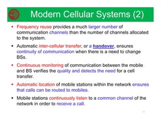
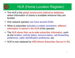
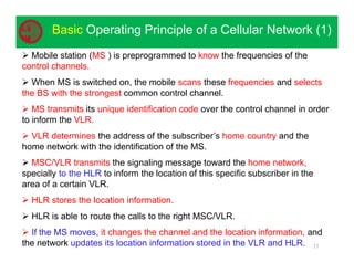
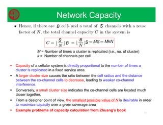
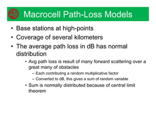
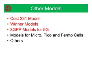
40. • Expressing the received power in dBm and
dBW
• Pr(d) (dBm) = 10 log [Pr(d0)] + 20log(d0/d)
where d = d0 = df and Pr(d0) is in units of mW
• Pr(d) (dBW) = 10 log [Pr(d0)] + 20log(d0/d)
where d = d0 = df and Pr(d0) is in units of watts
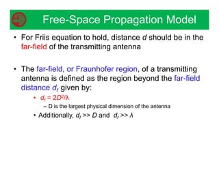
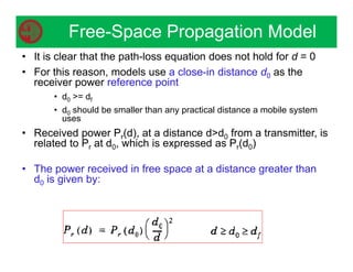
Free-Space Propagation Model
• Reference distance d0 for practical systems:
• For frequncies in the range 1-2 GHz
– 1 m in indoor environments
– 100m-1km in outdoor environments

41. • The average large-scale path
loss for an arbitrary T-R
separation is expressed as a
function of distance by using a
path loss exponent n:
– The value of n depends on the
propagation environment: for
free space it is 2; when
obstructions are present it has
a larger value.
= Average large-scale
path-loss at a distance d
)
log(
10
)
(
)
(
)
(
0
0
0
d
d
n
d
PL
dB
PL
d
d
d
PL
n











Long Distance Path Loss Model
)
(d
PL

42. Environment Path Loss Exponent, n
Free space 2
Urban area cellular radio 2.7 to 3.5
Shadowed urban cellular radio 3 to 5
In building line-of-sight 1.6 to 1.8
Obstructed in building 4 to 6
Obstructed in factories 2 to 3
Path Loss Exponent for Different
Environments

43. • Previous Equation does not
consider the fact that the
surrounding environment may
be vastly different at two
locations having the same T-R
separation
• This leads to measurements
that are different than the
predicted values obtained using
the above equation
• Measurements show that for
any value d, the path loss PL(d)
in dBm at a particular location is
random and distributed normally
Log-normal Shadowing

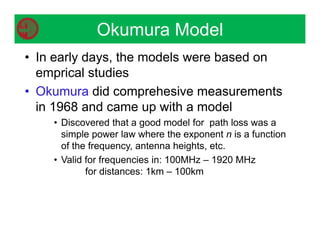
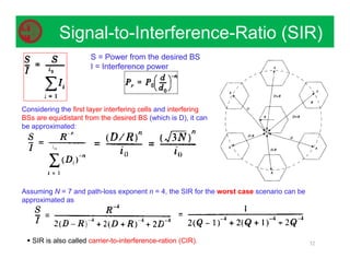
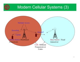
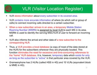
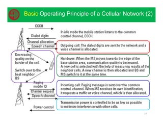
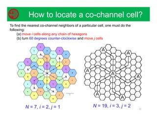
44. Xσ is a zero-mean Gaussian (normal) distributed random variable (in dB)
with standard deviation σ (also in dB)
Log-normal Shadowing - Path Loss
)
(d
PL

 X
d
d
n
d
PL
X
d
PL
dB
d
PL 



 )
log(
10
)
(
)
(
]
[
)
(
0
0
Then adding this random factor:
denotes the average large-scale path loss (in dB) at a distance d
)
( 0
d
PL is usually computed assuming free space propagation model between
transmitter and d0 (or by measurement)

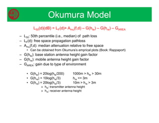
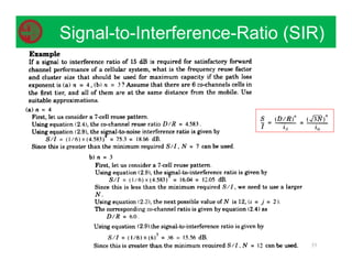
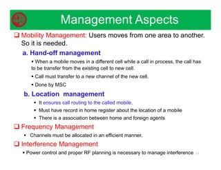
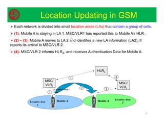
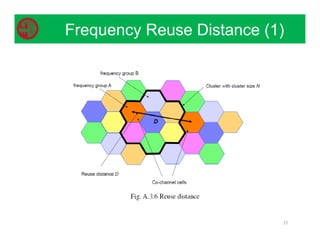
45. Log-normal Shadowing - Received Power
• The received power in log-normal shadowing
environment is given by the following formula
The picture can't be displayed.












]
[
)
log(
10
]
)[
(
]
[
]
)[
(
]
[
]
)[
(
0
0 dB
X
d
d
n
dB
d
PL
dBm
P
dB
d
PL
dBm
P
dBm
d
P
t
t
r


46. Macrocell Path-Loss Models
• Base stations at high-points
• Coverage of several kilometers
• The average path loss in dB has normal
distribution
• Avg path loss is result of many forward scattering over a
great many of obstacles
– Each contributing a random multiplicative factor
– Converted to dB, this gives a sum of random variable
• Sum is normally distributed because of central limit
theorem

47. • In early days, the models were based on
emprical studies
• Okumura did comprehesive measurements
in 1968 and came up with a model
• Discovered that a good model for path loss was a
simple power law where the exponent n is a function
of the frequency, antenna heights, etc.
• Valid for frequencies in: 100MHz – 1920 MHz
for distances: 1km – 100km
Okumura Model

48. Okumura Model
L50(d)(dB) = LF(d)+ Amu(f,d) – G(hte) – G(hre) – GAREA
– L50: 50th percentile (i.e., median) of path loss
– LF(d): free space propagation pathloss
– Amu(f,d): median attenuation relative to free space
• Can be obtained from Okumura’s emprical plots (Book: Rappaport)
– G(hte): base station antenna height gain factor
– G(hre): mobile antenna height gain factor
– GAREA: gain due to type of environment
• G(hte) = 20log(hte/200) 1000m hte 30m
• G(hre) = 10log(hre/3) hre = 3m
• G(hre) = 20log(hre/3) 10m hre 3m
» hte: transmitter antenna height
» hre: receiver antenna height

49. • Valid from 150MHz to 1500MHz
• A standard formula
• For urban areas the formula is:
L50(urban,d)(dB) = 69.55 + 26.16logfc - 13.82loghte – a(hre) + (44.9 – 6.55loghte)logd
where
fc is the ferquency in MHz
hte is effective transmitter antenna height in meters (30-200m)
hre is effective receiver antenna height in meters (1-10m)
d is T-R separation in km
a(hre) is the correction factor for effective mobile antenna height which is a
function of coverage area
a(hre) = (1.1logfc – 0.7)hre – (1.56logfc – 0.8) dB
for a small to medium sized city
Hata Model

50. • Cost 231 Model
• Winner Models
• 3GPP Models for 5G
• Models for Micro, Pico and Femto Cells
• Others
Other Models

51. 52
Signal-to-Interference-Ratio (SIR)
S = Power from the desired BS
I = Interference power
Assuming N = 7 and path-loss exponent n = 4, the SIR for the worst case scenario can be
approximated as
Considering the first layer interfering cells and interfering
BSs are equidistant from the desired BS (which is D), it can
be approximated:
 SIR is also called carrier-to-interference-ration (CIR).

52. 53
Signal-to-Interference-Ratio (SIR)

53. Coping with Increasing Capacity
54
 Add new channels
– Not all channels used to start with
 Frequency borrowing
– Taken from adjacent cells by
congested cells
– Or assign frequencies dynamically
 Cell splitting
– Non-uniform distribution of
topography and traffic
– Smaller cells in high use areas
• More frequent handoff
• More base stations

54. Coping with Increasing Capacity
55
 Cell Sectoring
– Cell divided into wedge shaped sectors
– 3-6 sectors per cell
– Each sector with own channel set
• Subsets of cell’s channels
– Directional antennas
 Microcells
– Move antennas from tops of hills and large buildings to
tops of small buildings and sides of large buildings
• Even lamp posts
– Form microcells
– Reduced power
– Good for city streets, along roads and inside large
buildings

55. Cell Splitting (1)
56

56. Cell Splitting (2)
57

57. Cell Sectorization
58
• Scctoring reduces interference from co-channel cells.
• 120° sectoring, out of the 6 co-channel cells in the first tier, only 2 interfere with the
center cell.
• If omnidirectional antennas were used at each base station, all 6 co-channel cells
would interfere with the center cell.
5
5
5
5
5
5
7
6
1
4
2
3
Omnidirectional Sectorized Directive
90
270
180
150
120
30
300
240
210 330
60
0
90
270
180
150
120
30
300
240
210 330
60
0
90
270
180
150
120
30
300
240
210 330
60
0

58. Handoff
59
Handoffs are the function of one cell handing over the communication link between
itself and a MS as the MS moves out of the boundary of its region into the boundary of
an adjacent cell.
Hard handover is one in which the channel
in the source cell is released and only then
the channel in the target cell is engaged.
Thus the connection to the source is broken
before or 'as' the connection to the target is
made—for this reason such handovers are
also known as break-before-make.
Soft handover is one in which the channel
in the source cell is retained and used for a
while in parallel with the channel in the
target cell. In this case the connection to the
target is established before the connection
to the source is broken, hence this handover
is called make-before-break.

59. Multiple Access Techniques
60
Frequency Division Multiple Access
- when the subscriber enters another
cell a unique frequency is assigned to
the user; used in analog systems
Time Division Multiple Access
- each subscriber is assigned a time slot
to send/receive a data burst; is used in
digital systems
Code Division Multiple Access
- each subscriber is assigned a code
which is used to multiply the signal sent
or received by the subscriber