1. letters to nature
.............................................................. agreement over nearly 35 Myr.
Mercury’s capture into the 3/2 Owing to the chaotic evolution, the density function of the 1,000
solutions over 4 Gyr is a smooth function (Fig. 1), similar, but not
spin-orbit resonance as a equal, to a gaussian curve14. The mean value of the eccentricity eLA04
is slightly higher than eBVW50 and eBRE74 ; but the main difference is a
result of its chaotic dynamics much wider range for the eccentricity variations, from nearly zero to
more than 0.45. The planet eccentricity can now increase beyond e 3/
Alexandre C. M. Correia1,2 Jacques Laskar2 2 during its history. Even if these episodes do not last for a long time,
they will allow additional capture into the 3/2 spin-orbit resonance.
1
´ ´
Departamento de Fısica da Universidade de Aveiro, Campus Universitario de For each of these 1,000 orbital motions of Mercury, we have
Santiago, 3810-193 Aveiro, Portugal numerically integrated the rotational motion of the planet, taking
2
`
Astronomie et Systemes Dynamiques, IMCCE-CNRS UMR8028, Observatoire into account the resonant terms of equation (2), for p ¼ k/2 with
de Paris, 77 Avenue Denfert-Rochereau, 75014 Paris, France k ¼ 1,…,10, the tidal dissipation, and the planetary perturbations,
.............................................................................................................................................................................
starting at t 0 ¼ 24 Gyr, with a rotation period of 20 days. Because e
Mercury is locked into a 3/2 spin-orbit resonance where it rotates is not constant, the ratio x(t) of the rotation rate of the planet to its
three times on its axis for every two orbits around the sun1–3. The mean motion n will tend towards a limit value xl ðtÞ (see Methods)
~
stability of this equilibrium state is well established4–6, but our that is similar to an averaged value of x l(e(t)), and capture into
understanding of how this state initially arose remains unsatis- resonance can now occur in various ways.
factory. Unless one uses an unrealistic tidal model with constant Type I is the classical case, where e , e p (Fig. 2a). It is only in this
torques (which cannot account for the observed damping of the case that the probability formula of Goldreich and Peale5 will apply.
libration of the planet) the computed probability of capture into In type II, the eccentricity oscillates around e p at the time when the
3/2 resonance is very low (about 7 per cent)5. This led to the
spin rate x(t) decreases towards p. The tidal dissipation thus drives
proposal that core–mantle friction may have increased the
x(t) several times across p, greatly increasing the probability of
capture probability, but such a process requires very specific
capture (Fig. 2b). Types I and II can only occur in the first few Myr,
values of the core viscosity7,8. Here we show that the chaotic
as the spin rate decreases from faster rotations. We distinguish these
evolution of Mercury’s orbit can drive its eccentricity beyond
cases from type III, where the planet is not initially captured into
0.325 during the planet’s history, which very efficiently leads to
its capture into the 3/2 resonance. In our numerical integrations
of 1,000 orbits of Mercury over 4 Gyr, capture into the 3/2 spin-
orbit resonant state was the most probable final outcome of the
planet’s evolution, occurring 55.4 per cent of the time.
Tidal dissipation will drive the rotation rate of the planet towards
a limit equilibrium value x l(e)n depending on the eccentricity e and
on the mean motion n (see Methods). In a circular orbit (e ¼ 0) this
equilibrium coincides with synchronization (x l (0) ¼ 1), but
x l(e 0) ¼ 1.25685 for the present value of Mercury’s eccentricity
(e 0 ¼ 0.206), while the equilibrium rotation rate 3n/2 is achieved
for e 3/2 ¼ 0.284927. In their seminal work5, Goldreich and Peale
assumed that Mercury passed through the 3/2 resonance during its
initial spin-down. They derived an analytical estimate of the capture
probability into the 3/2 resonance and found P 3/2 ¼ 6.7% for the
eccentricity e 0. With the updated value of the momentum of inertia9
ðB 2 AÞ=C . 1:2 £ 1024 ; this probability increases to 7.73%, and
our numerical simulations with the same setting give P 3/2 ¼ 7.10%
with satisfactory agreement.
In fact, using the present value of the eccentricity of Mercury is
questionable, as the eccentricity undergoes strong variations in
time, owing to planetary secular perturbations. Assuming a random
date for the crossing of the 3/2 resonance for 2,000 orbits, we
found numerically PBVW50 ¼ 3:92% and PBRE74 ¼ 5:48% for these-
3=2 3=2
cular (averaged) solutions of Brouwer and Van Woerkom10 and
Bretagnon11. It should be stressed that with the regular quasiper-
iodic solutions BVW50 or BRE74, as for the fixed value of the
eccentricity e 0, the 3/2 resonance can be crossed only once, because
e , e 3/2. This will no longer be the case with a complete solution for
Mercury’s orbit that takes into account its chaotic evolution12,13. In
this case, Mercury’s eccentricity can exceed the characteristic value
e 3/2 (Fig. 1), and additional capture into resonance can occur.
To check this new scenario, it is not possible to use a single orbital
solution because, owing to its chaotic behaviour, the motion cannot
be predicted precisely beyond a few tens of millions of years. We
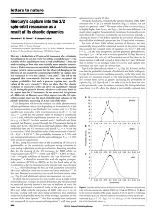
have thus performed a statistical study of the past evolutions of Figure 1 Probability density function of Mercury’s eccentricity. Values are computed over
Mercury’s orbit, with the integration of 1,000 orbits over 4 Gyr in 4 Gyr for the two quasiperiodic solutions BVW50 (ref. 10) (a) and BRE74 (ref. 11) (b) and
the past, starting with very close initial conditions. This statistical for the numerical integration of the secular equations of refs 12 and 14 for 1,000 close
study was made possible by the use of the averaged equations for the initial conditions (LA04, c). The mean values of the eccentricity in these solutions are
motion of the Solar System12,13 that have recently been readjusted respectively eBVW50 ¼ 0:177; eBRE74 ¼ 0:181; and eLA04 ¼ 0:198: The vertical dotted
and compared to recent numerical integrations14, with very good line is the characteristic value e 3/2.
848 ©2004 Nature Publishing Group NATURE | VOL 429 | 24 JUNE 2004 | www.nature.com/nature

2. letters to nature
Table 1 Critical eccentricity e c(p) for the resonance p
p e c(p)
.............................................................................................................................................................................
1/1 –
3/2 0.000026
2/1 0.004602
5/2 0.024877
3/1 0.057675
7/2 0.095959
4/1 0.135506
9/2 0.174269
5/1 0.211334
.............................................................................................................................................................................
If e , e c(p), the resonance p becomes unstable, and the solution may escape the resonance.
The critical eccentricity e c (p) is obtained by the resolution of ½QðeÞp 2 NðeÞŠ=Hðp; eÞ ¼
ð3=2KÞ n½ðB 2 AÞ=CŠ:
solutions are very close in the vicinity of the origin. Among the
solutions captured into the 3/2 resonance, we can distinguish 31
solutions of type I, 168 of type II and 355 of type III (Fig. 2).
With the consideration of the chaotic evolution of the eccentri-
city of Mercury, we thus show that with a realistic tidal dissipative
model that properly accounts for the damping of the libration of the
planet, and without the need for some additional core–mantle
friction, the present 3/2 resonant state is the most probable outcome
for the planet.
Additionally, from the present state of the planet, we can derive
an interesting constraint on its past evolution. Of all 554 orbits
trapped into the 3/2 resonance, for 521 of them (94.0%) Mercury’s
eccentricity exceeded 0.325 in the past 4 Gyr. The conditional
Figure 2 Typical cases of capture into the 3/2 resonance. The rotation rate x(t ) (bold
probability that Mercury’s eccentricity exceeded 0.325, given that
curve) and limit value x l (e(t )) (dotted curve) are plotted versus time (Gyr). a, Type I is the
its rotation is trapped into the 3/2 resonance, is thus 94.0%. The 3/2
classical case5: As e , e 3/2, the limit value x l is always lower than 3/2. b, In Type II, at
resonant state of Mercury thus becomes an observational clue that
the time when x reaches the resonant value 3/2, e is oscillating around e 3/2, leading to
the chaotic evolution of the planet orbit led its eccentricity beyond
multiple crossings of the resonance, with ultimately a capture. c, Type III corresponds to
0.325 over its history.
solutions that have not been captured during the initial crossing of the resonance, but later
The largest unknown in this study remains the dissipation factor
on, as the eccentricity increases beyond e 3/2.
k 2/Q of K (equation (4)) (ref. 15). A stronger dissipation would
increase the probability of capture into the 3/2 resonance, because
x(t) would follow more closely x l(e(t)) (Fig. 2), whereas lower
resonance p; but later on, as the orbital elements evolve, the
dissipation would slightly decrease the capture probability. This study
eccentricity increases beyond e p, and tidal dissipation accelerates
should apply more generally to any extrasolar planet or satellite
the spin rate beyond p, leading to additional capture (Fig. 2c).
whose eccentricity is forced by planetary perturbations. A
Over 1,000 orbits, a few were initially trapped in high-order
resonances (one in 7/2, one in 4/1, two in 9/2 and three in 5/1), but
Methods
these were associated with high values of the planet’s eccentricity. As Tidal dissipation and core–mantle friction will drive Mercury’s obliquity (the angle
the eccentricity decreased these resonances became unstable, and between the equator and the orbital plane) close to zero. For zero-degree obliquity, and in
none of these high-order resonances survived. They did eventually the absence of dissipation, the averaged equation for the rotational motion near resonance
get trapped for a long time into the 5/2 resonance, but even that did p (where p is a half-integer) is4,5:
not survive over the full history of the planet. Indeed, the stability of 3 B2A
x¼2 n
_ Hðp; eÞ sin2ð‘ 2 pMÞ ð2Þ
the resonances depends on the eccentricity of Mercury, and except 2 C
_ =n is the ratio of the rotation rate to the mean motion
where ‘ is the rotational angle, x ¼ ‘
for the 1/1 resonance, the resonances may become unstable for very
n, M is the mean anomaly and H(p, e) are Hansen coefficients5,16. The moments of inertia
small values of the eccentricity (Table 1). are A , B , C, with C ¼ ymR 2, where m and R are the mass and radius of the planet, and
We followed all 1,000 solutions, starting from 24 Gyr, until they y is a structure constant.
reached the present date or were captured into the 2/1, 3/2 or 1/1 Tidal models independent of the frequency (constant-Q models) do not account for
the damping of the amplitude of libration that is at present observed on Mercury5,17.
resonances. Unlike in previous studies, we found that capture into
Moreover, these models introduce discontinuities into the equations and can thus be
the 1/1 resonance is possible, because the eccentricity of Mercury considered as unrealistic approximations for slow rotating bodies18. Therefore, we use here
may decrease to very low values at which capture can occur and the for slow rotations a viscous tidal model, with a linear dependence on the tidal frequency.
resonance remain stable. Over 554 solutions that were captured into Its contribution to the rotation rate is given by5,18,19,20:
the 3/2 resonance, a single one, initially captured at 23.995 Gyr, x ¼ 2K½QðeÞx 2 NðeÞŠ
_ ð3Þ
escaped from resonance at about 22.396 Gyr. The solution then got with QðeÞ ¼ ð1 þ 3e2 þ 3e4 =8Þ=ð1 2 e2 Þ9=2 ; NðeÞ ¼ ð1 þ 15e2 =2 þ 45e4 =8 þ 5e6 =16Þ=ð1 2
trapped into the 1/1 resonance at 22.290 Gyr, capture that was e2 Þ6 ; and
favoured by the very low eccentricity required to destabilize the 3/2 k2 R 3 m 0
K ¼ 3n ð4Þ
resonance (Table 1). Out of the 56 solutions initially trapped into yQ a m
the 2/1 resonance, ten were destabilized, and only two of them were where k 2 and Q are the second Love number and the quality factor, while a, m and m 0 are
further captured, one into the 3/2 resonance, and one into the 1/1 the semi-major axis, the mass of the planet and the solar mass, respectively. Equilibrium is
achieved when x ¼ 0; that is, for constant e, when x ¼ x l(e) ¼ N(e)/Q(e).
_
resonance. Globally, we obtained a final capture probability: For a non-constant eccentricity e(t), the limit solution of equation (3) is no longer
x l(e), but more generally:
P1=1 ¼ 2:2%; P3=2 ¼ 55:4%; P2=1 ¼ 3:6% ð1Þ ðt
xl ðtÞ ¼ xð0Þ þ K NðeðtÞÞgðtÞdt =gðtÞ
~ ð5Þ
The remaining 38.8% non-resonant solutions end with nearly the 0
Ðt
same final rotation rate of x f ¼ 1.21315, because all the orbital where gðtÞ ¼ expðK 0 QðeðtÞÞdtÞ:
NATURE | VOL 429 | 24 JUNE 2004 | www.nature.com/nature
©2004 Nature Publishing Group 849

3. letters to nature
Using y ¼ 0.3333, k 2 ¼ 0.4 and Q ¼ 50 (refs 15, 21), we have materials manifests itself in their reaction to an external mag-
K ¼ 8.45324 £ 1027 yr21. Assuming an initial rotation period of Mercury of 10 h, we netic field—in an antiferromagnet, the exchange interaction leads
estimated that the time needed to despin the planet to the slow rotations would be about
300 million years. This is why we started our integrations in the slow-rotation regime, with
to zero net magnetization. The related absence of a net angular
a rotation period of 20 days (x 4.4) and a starting time of 24 Gyr, although these values momentum should result in orders of magnitude faster AFM spin
are not critical. dynamics6,7. Here we show that, using a short laser pulse, the
Received 12 March; accepted 4 May 2004; doi:10.1038/nature02609. spins of the antiferromagnet TmFeO3 can indeed be manipulated
1. Pettengill, G. H. Dyce, R. B. A radar determination of the rotation of the planet Mercury. Nature
on a timescale of a few picoseconds, in contrast to the hundreds of
206, 1240 (1965). picoseconds in a ferromagnet8–12. Because the ultrafast dynamics
2. McGovern, W. E., Gross, S. H. Rasool, S. I. Rotation period of the planet Mercury. Nature 208, 375 of spins in antiferromagnets is a key issue for exchange-biased
(1965). devices13, this finding can expand the now limited set of appli-
3. Colombo, G. Rotation period of the planet Mercury. Nature 208, 575 (1965).
4. Colombo, G. Shapiro, I. I. The rotation of the planet Mercury. Astrophys. J. 145, 296–307 (1966).
cations for AFM materials.
5. Goldreich, P. Peale, S. J. Spin orbit coupling in the Solar System. Astron. J. 71, 425–438 (1966). To deflect the magnetization of a ferromagnet from its equili-
6. Counselman, C. C. Shapiro, I. I. Spin-orbit resonance of Mercury. Symp. Math. 3, 121–169 (1970). brium, a critical field H FM H A of the order of the effective
cr
7. Goldreich, P. Peale, S. J. Spin-orbit coupling in the solar system 2. The resonant rotation of Venus.
anisotropy field is required. In contrast, the response of an anti-
Astron. J. 72, 662–668 (1967).
8. Peale, S. J. Boss, A. P. A spin-orbit constraint on the viscosity of a Mercurian liquid core. J. Geophys. ferromagnet to an applied field remains pffiffiffiffiffiffiffiffiffiffiffiffiffiffi
very weak before the
Res. 82, 743–749 (1977). exchanged-enhanced critical field H AFM H A H ex is reached. In
cr
9. Anderson, J. D., Colombo, G., Espsitio, P. B., Lau, E. L. Trager, G. B. The mass, gravity field, and most materials the exchange field H ex . H A (H A , 1 T,
.
ephemeris of Mercury. Icarus 71, 337–349 (1987).
10. Brouwer, D. Van Woerkom, A. J. J. The secular variations of the orbital elements of the principal
H ex 100 T) and thus H AFM . H FM : This difference is related to
cr . cr
planets. Astron. Pap. Am. Ephem. XIII, part II, 81–107 (1950). the fact that in an antiferromagnet, no angular momentum is
` ´ `
11. Bretagnon, P. Termes a longue periodes dans le systeme solaire. Astron. Astrophys. 30, 141–154 (1974). associated with the AFM moment. This large rigidity of an anti-
12. Laskar, J. The chaotic motion of the solar system. Icarus 88, 266–291 (1990). ferromagnet to an external field also shows up in the magnetic
13. Laskar, J. Large-scale chaos in the Solar System. Astron. Astrophys. 287, L9–L12 (1994).
14. Laskar, J. et al. Long term evolution and chaotic diffusion of the insolation quantities of Mars. Icarus
resonance frequency 14 , where spin excitations start at q
pffiffiffiffiffiffiffiffiffiffiffiffiffiffi
(in the press). g H A H ex : This is in contrast to q gH A in a ferromagnet,
15. Spohn, T., Sohl, F., Wieczerkowski, K. Conzelmann, V. The interior structure of Mercury: what we which can result in a difference of more than two orders of
know, what we expect from BepiColombo. Planet. Space Sci. 49, 1561–1570 (2001).
magnitude.
16. Hansen, P. A. Entwickelung der products einer potenz des radius vectors mit dem sinus oder cosinus
eines vielfachen der wahren anomalie in reihen. Abhandl. K. S. Ges. Wissensch. IV, 182–281 (1855). Indeed, dynamical many-body theory calculations15 show a
17. Murray, C. D. Dermott, S. F. Solar System Dynamics (Cambridge Univ. Press, Cambridge, 1999). possibility of AFM dynamics with a time constant of a few
´
18. Correia, A. C. M. Laskar, J. Neron de Surgy, O. Long term evolution of the spin of Venus. I. Theory. femtoseconds only. Experimentally, the ultrafast dynamics of an
Icarus 163, 1–23 (2003).
19. Munk, W. H. MacDonald, G. J. F. The Rotation of the Earth; A Geophysical Discussion (Cambridge
antiferromagnet is still an intriguing question. The problem how-
Univ. Press, Cambridge, 1960). ever is far from trivial, as there is no straightforward method
20. Kaula, W. Tidal dissipation by solid friction and the resulting orbital evolution. J. Geophys. Res. 2, for the manipulation and detection of spins in AFM materials.
661–685 (1964). Therefore, an appropriate mechanism should be found that would
21. Yoder, C. F. Astrometric and geodetic properties of Earth and the Solar System. Glob. Earth Physics: A
Handbook of Physical Constants 1–31 (American Geophysical Union, Washington DC, 1995).
deflect the AFM moments on a timescale down to femtoseconds,
and this change should subsequently be detected on the same
Acknowledgements This work was supported by PNP-CNRS, Paris Observatory CS, and timescale.
¸˜ ˆ
Fundacao para a Ciencia e a Technologia, POCTI/FNU, Portugal. The numerical computations The solution to this problem can be found in the magnetocrystal-
were made at IDRIS-CNRS, and Paris Observatory. Authors are listed in alphabetic order.
line anisotropy. Indeed, a rapid change of this anisotropy can lead,
via the spin–lattice interaction, to a reorientation of the spins11,12.
Competing interests statement The authors declare that they have no competing financial
interests.
Such anisotropy change, in turn, can be induced by a short
femtosecond laser pulse in a material with a strong temperature-
Correspondence and requests for materials should be sent to J.L. (Laskar@imcce.fr). dependent anisotropy. The subsequent reorientation of the spins
can be detected with the help of time-resolved linear magnetic
birefringence16, which enables us to follow the change of the
direction of spins in antiferromagnets, similar to the Faraday and
Kerr effects in ferromagnets.
.............................................................. The rare-earth orthoferrites RFeO3 (where R indicates a rare-
earth element) investigated here are known for a strong tempera-
Laser-induced ultrafast spin ture-dependent anisotropy17,18. These materials crystallize in an
orthorhombically distorted perovskite structure, with a space-
reorientation in the antiferromagnet group symmetry D16 (Pbnm). The iron moments order antiferro-
2h
magnetically, as shown in Fig. 1, but with a small canting of the
TmFeO3 spins on different sublattices. The temperature-dependent aniso-
tropy energy has the form19,20:
A. V. Kimel1, A. Kirilyuk1, A. Tsvetkov1, R. V. Pisarev2 Th. Rasing1
FðTÞ ¼ F0 þ K 2 ðTÞsin2 v þ K 4 sin4 v ð1Þ
1
NSRIM Institute, University of Nijmegen, Toernooiveld 1, 6525 ED Nijmegen,
The Netherlands where v is the angle in the x–z plane between the x axis and the AFM
2
Ioffe Physico-Technical Institute, 194021 St.-Petersburg, Russia moment G, see Fig. 1, and K 2 and K 4 are the anisotropy constants of
............................................................................................................................................................................. second and fourth order, respectively. Applying equilibrium con-
All magnetically ordered materials can be divided into two ditions to equation (1) yields three temperature regions corre-
primary classes: ferromagnets1,2 and antiferromagnets3. Since sponding to different spin orientations:
ancient times, ferromagnetic materials have found vast appli-
G4 ðGx F z Þ : v ¼ 0; T $ T 2
cation areas4, from the compass to computer storage and more
recently to magnetic random access memory and spintronics5. In G2 ðGz F x Þ : v ¼ 1=2p; T # T 1
contrast, antiferromagnetic (AFM) materials, though represent-
ing the overwhelming majority of magnetically ordered
G24 : sin2 v ¼ K 2 ðTÞ=2K 4 ; T 1 # T # T 2 ð2Þ
materials, for a long time were of academic interest only. The
fundamental difference between the two types of magnetic where T 1 and T 2 are determined by the conditions K2(T 1) ¼ 22K 4
850 ©2004 Nature Publishing Group NATURE | VOL 429 | 24 JUNE 2004 | www.nature.com/nature