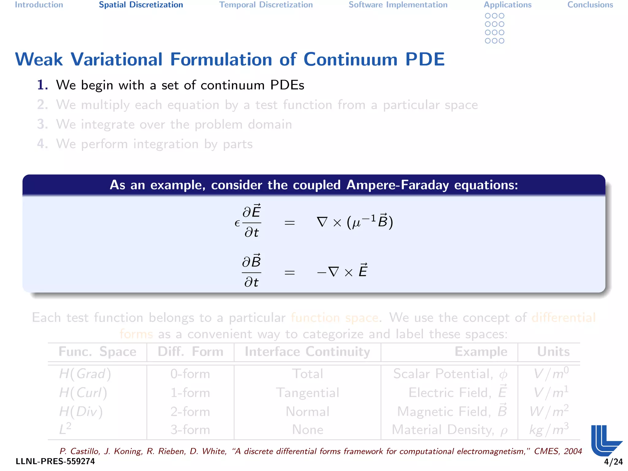
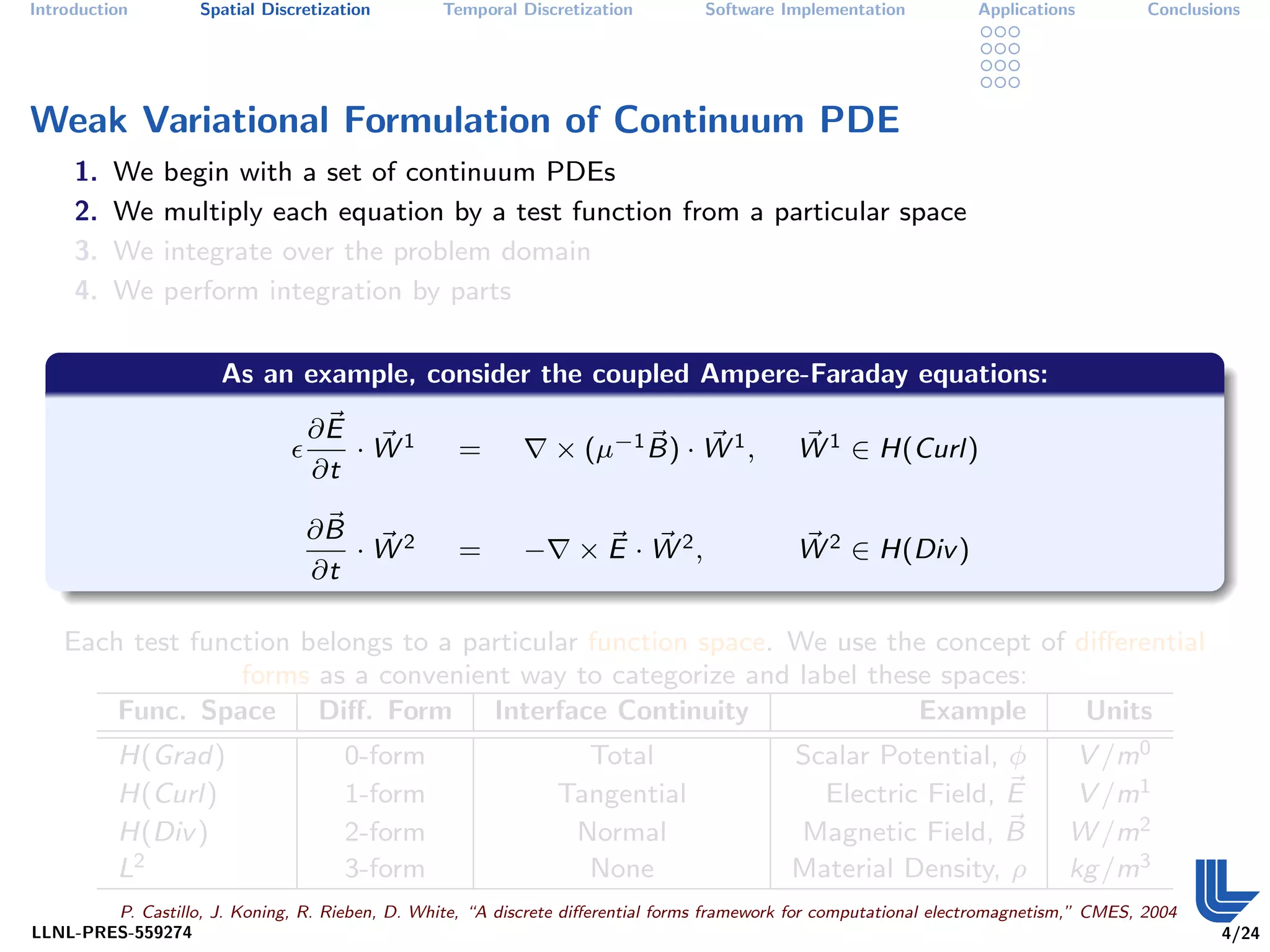
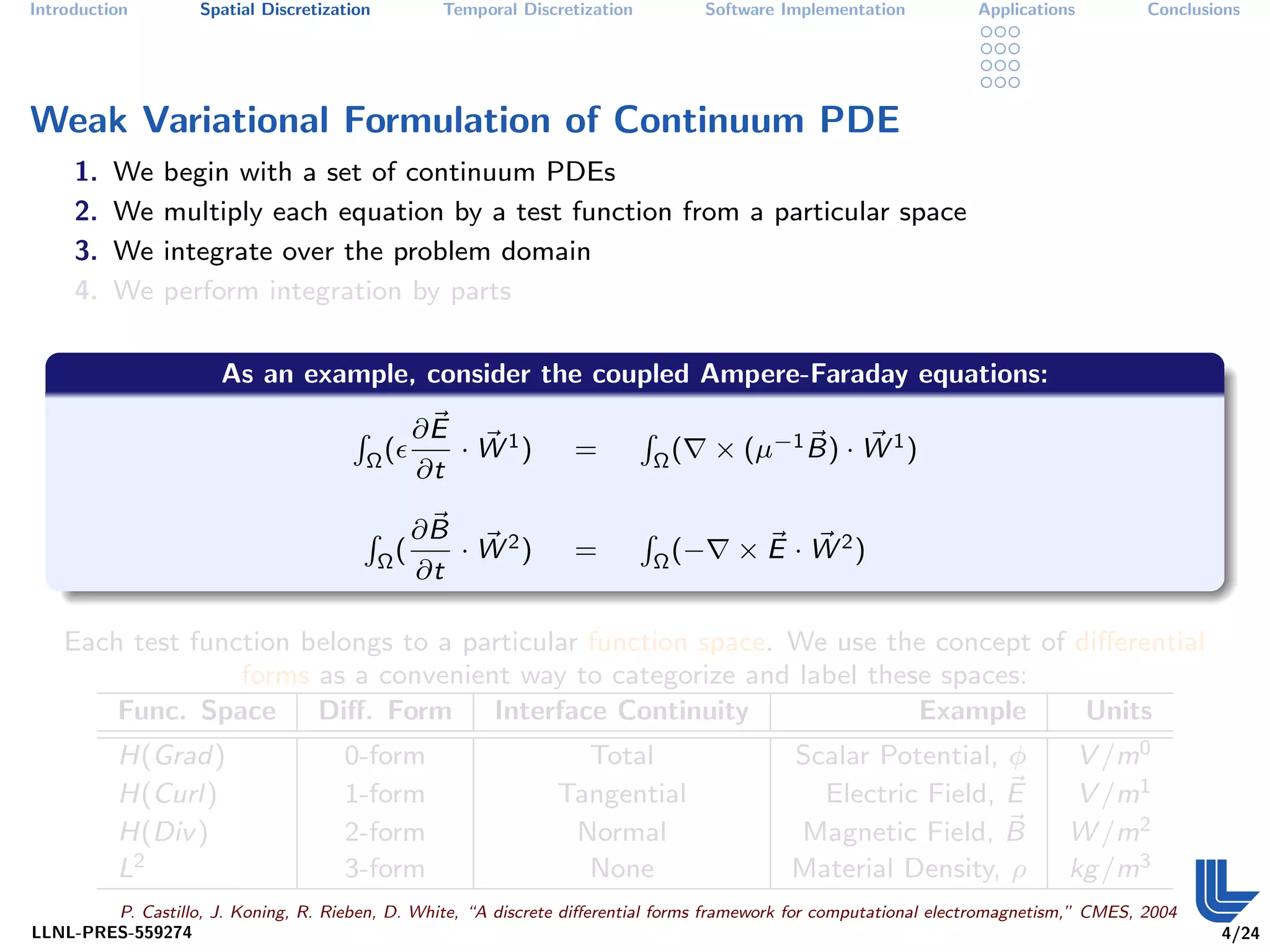
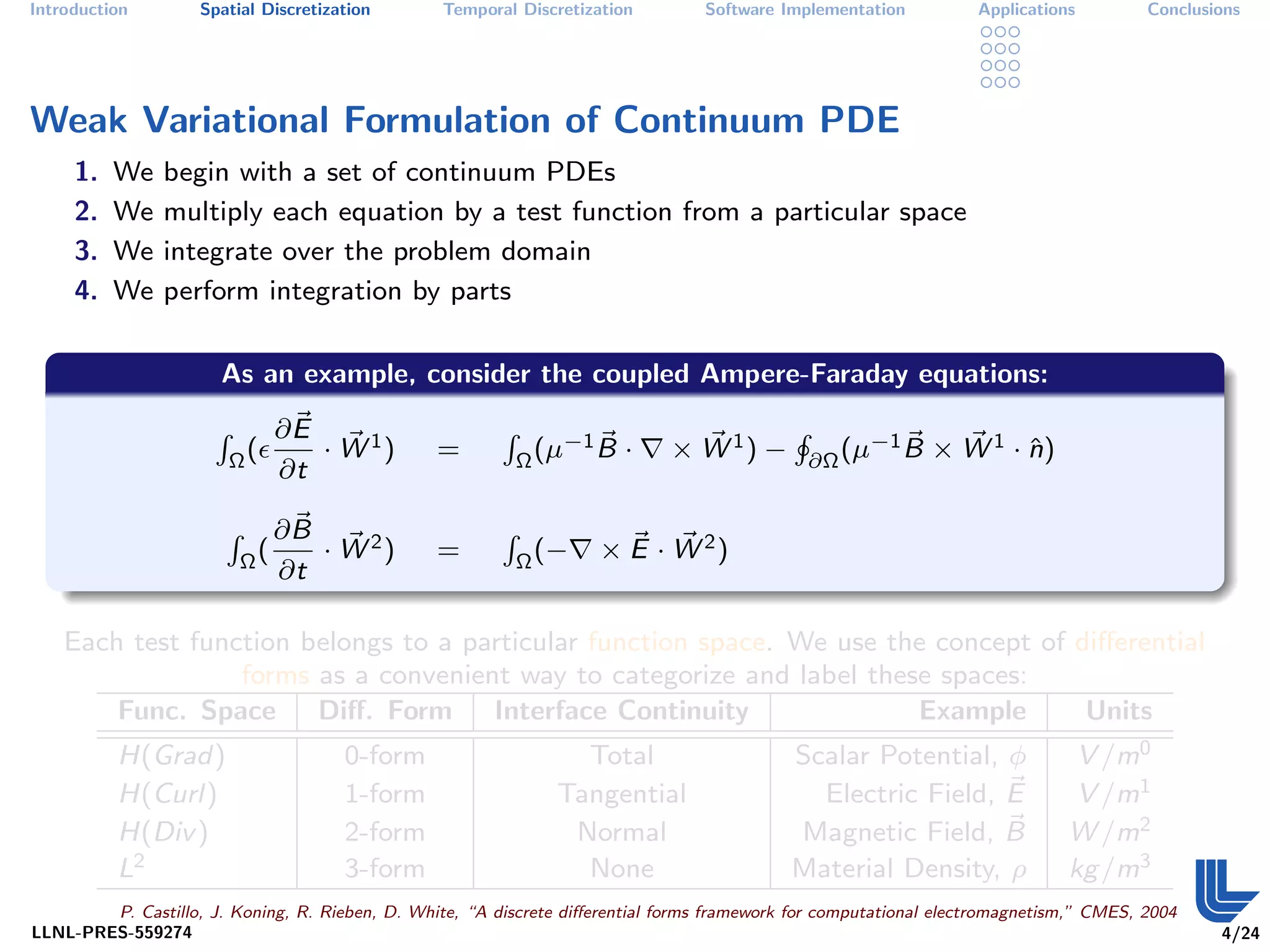
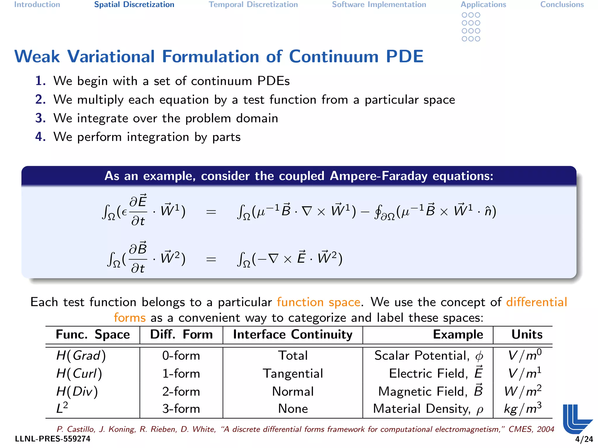
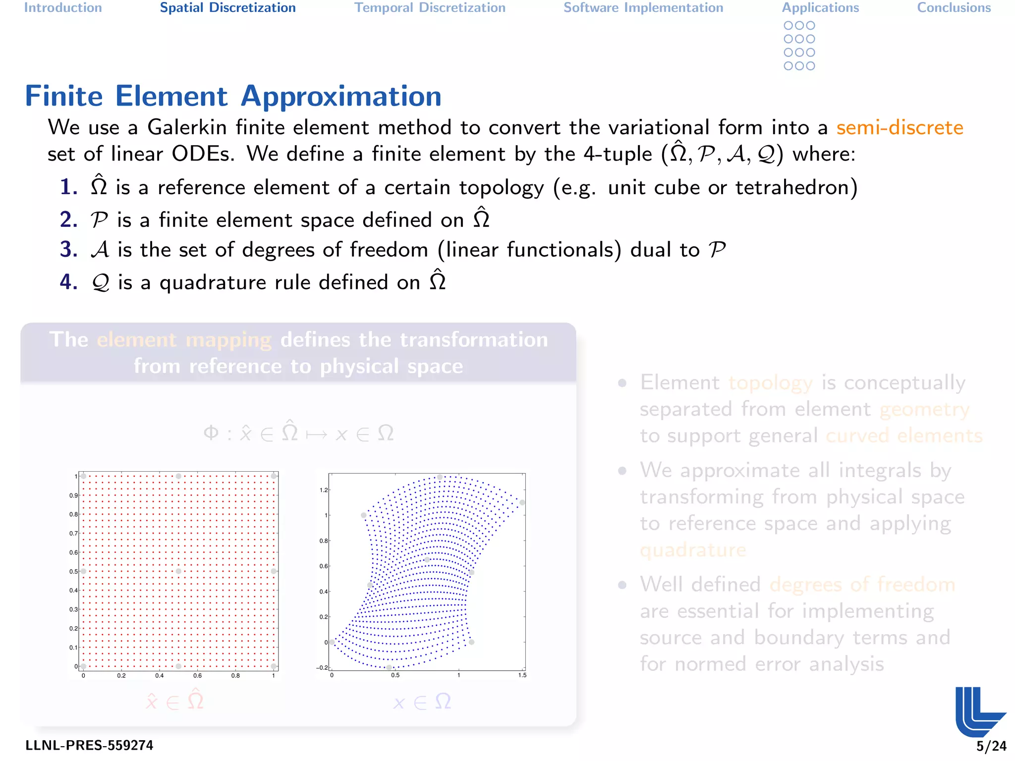
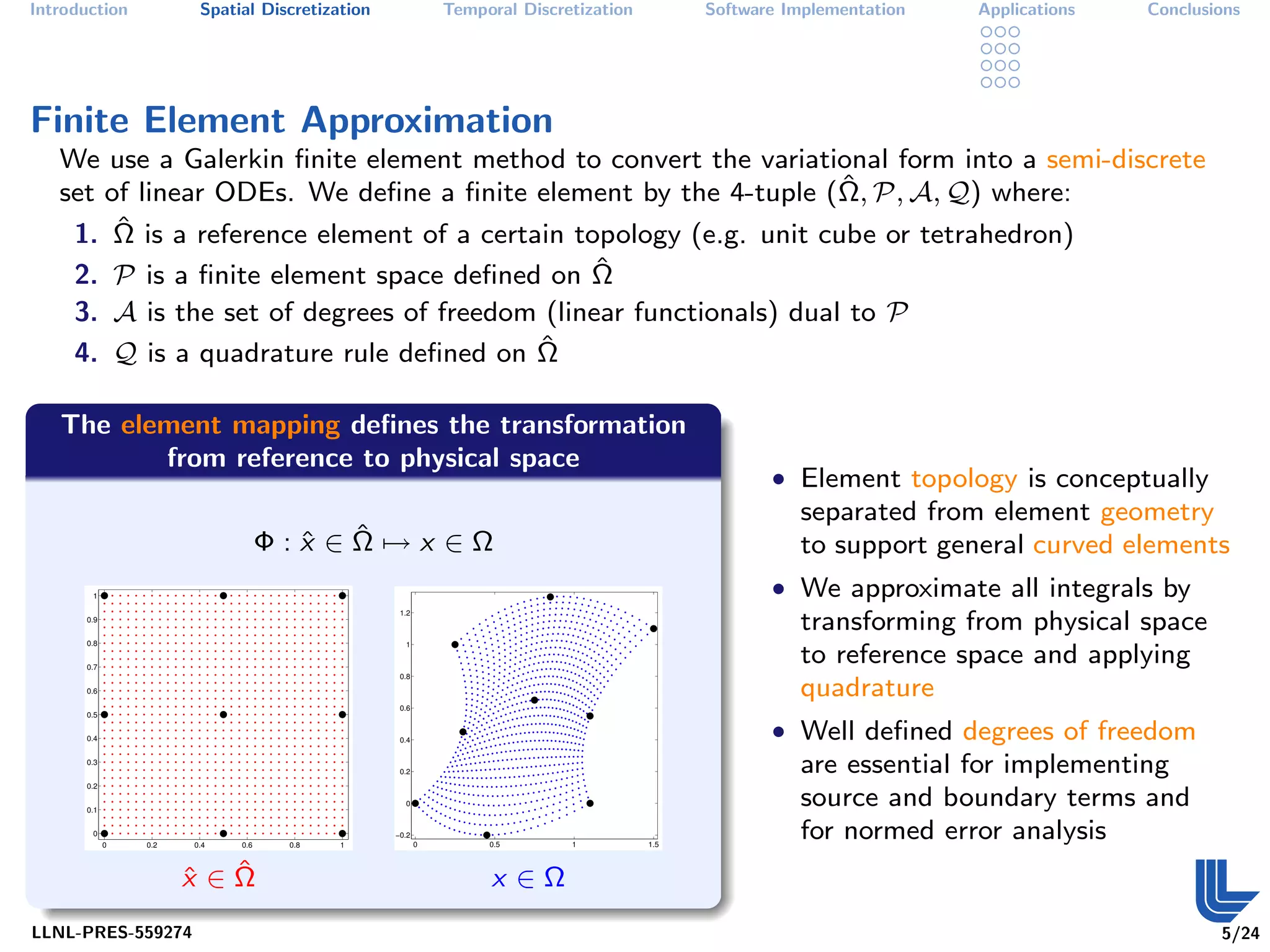
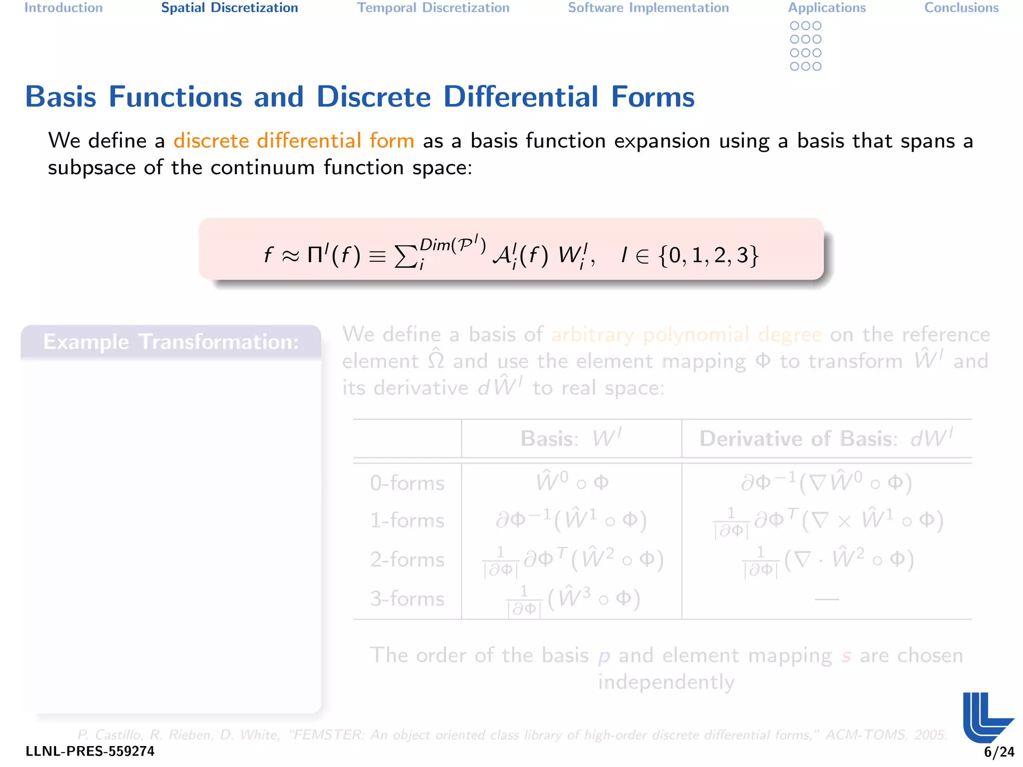
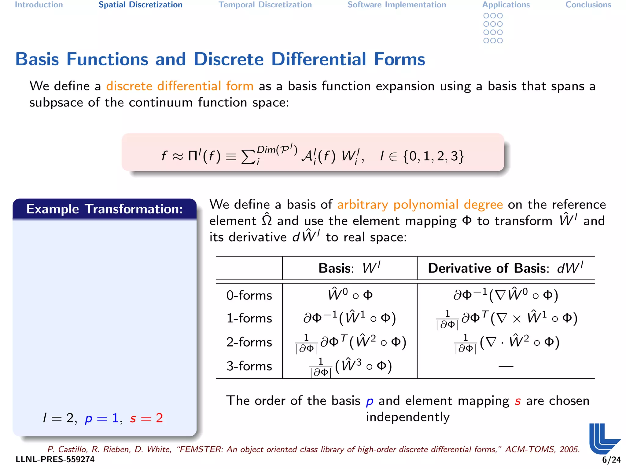
The document discusses high order finite element methods for computational physics from Lawrence Livermore National Laboratory's perspective. It introduces the weak variational formulation of partial differential equations, finite element approximation using a Galerkin method, and the use of discrete differential forms and basis functions to represent solutions. The goal is to develop robust, modular software for solving multi-physics problems on massively parallel architectures.

1. High Order Finite Elements For Computational Physics:
An LLNL Perspective
FEM 2012 Workshop
Estes Park, Colorado, June 4th, 2012
Robert N. Rieben
LLNL-PRES-559274
This work was performed under the auspices of the
U.S. Department of Energy by Lawrence Livermore
National Laboratory under contract
DE-AC52-07NA27344. Lawrence Livermore National
Security, LLC

2. Introduction Spatial Discretization Temporal Discretization Software Implementation Applications Conclusions
Acknowledgments
This is joint work with:
• P. Castillo
• V. Dobrev
• A. Fisher
• T. Kolev
• J. Koning
• G. Rodrigue
• M. Stowell
• D. White
LLNL-PRES-559274 2/24

3. Introduction Spatial Discretization Temporal Discretization Software Implementation Applications Conclusions
Motivation
Our goal is to model, and ultimately predict, the behavior of complex physical systems by
solving a set of coupled partial differential equations
Our simulation codes must:
• work on general unstructured 2D and 3D meshes
• run on massively parallel computing architectures
• be adaptable and extendable
We like high order algorithms because they:
• minimize numerical dispersion
• maximize FLOPS/byte (well suited for exascale platforms)
• often lead to more robust algorithms
We have adopted a general approach for solving PDEs using high order finite elements that:
• is implemented in modular software libraries
• has been integrated into production multi-physics codes
• forms the basis for new research codes founded on high order methods
LLNL-PRES-559274 3/24

4. Introduction Spatial Discretization Temporal Discretization Software Implementation Applications Conclusions
Weak Variational Formulation of Continuum PDE
1. We begin with a set of continuum PDEs
2. We multiply each equation by a test function from a particular space
3. We integrate over the problem domain
4. We perform integration by parts
As an example, consider the coupled Ampere-Faraday equations:
∂E
= × (µ−1 B)
∂t
∂B
= − ×E
∂t
Each test function belongs to a particular function space. We use the concept of differential
forms as a convenient way to categorize and label these spaces:
Func. Space Diff. Form Interface Continuity Example Units
H(Grad) 0-form Total Scalar Potential, φ V /m0
H(Curl) 1-form Tangential Electric Field, E V /m1
H(Div ) 2-form Normal Magnetic Field, B W /m2
L2 3-form None Material Density, ρ kg /m3
P. Castillo, J. Koning, R. Rieben, D. White, “A discrete differential forms framework for computational electromagnetism,” CMES, 2004
LLNL-PRES-559274 4/24

5. Introduction Spatial Discretization Temporal Discretization Software Implementation Applications Conclusions
Weak Variational Formulation of Continuum PDE
1. We begin with a set of continuum PDEs
2. We multiply each equation by a test function from a particular space
3. We integrate over the problem domain
4. We perform integration by parts
As an example, consider the coupled Ampere-Faraday equations:
∂E
· W1 = × (µ−1 B) · W 1 , W 1 ∈ H(Curl)
∂t
∂B
· W2 = − × E · W 2, W 2 ∈ H(Div )
∂t
Each test function belongs to a particular function space. We use the concept of differential
forms as a convenient way to categorize and label these spaces:
Func. Space Diff. Form Interface Continuity Example Units
H(Grad) 0-form Total Scalar Potential, φ V /m0
H(Curl) 1-form Tangential Electric Field, E V /m1
H(Div ) 2-form Normal Magnetic Field, B W /m2
L2 3-form None Material Density, ρ kg /m3
P. Castillo, J. Koning, R. Rieben, D. White, “A discrete differential forms framework for computational electromagnetism,” CMES, 2004
LLNL-PRES-559274 4/24

6. Introduction Spatial Discretization Temporal Discretization Software Implementation Applications Conclusions
Weak Variational Formulation of Continuum PDE
1. We begin with a set of continuum PDEs
2. We multiply each equation by a test function from a particular space
3. We integrate over the problem domain
4. We perform integration by parts
As an example, consider the coupled Ampere-Faraday equations:
∂E
· W 1) × (µ−1 B) · W 1 )
R R
Ω( = Ω(
∂t
∂B
· W 2) × E · W 2)
R R
Ω( = Ω (−
∂t
Each test function belongs to a particular function space. We use the concept of differential
forms as a convenient way to categorize and label these spaces:
Func. Space Diff. Form Interface Continuity Example Units
H(Grad) 0-form Total Scalar Potential, φ V /m0
H(Curl) 1-form Tangential Electric Field, E V /m1
H(Div ) 2-form Normal Magnetic Field, B W /m2
L2 3-form None Material Density, ρ kg /m3
P. Castillo, J. Koning, R. Rieben, D. White, “A discrete differential forms framework for computational electromagnetism,” CMES, 2004
LLNL-PRES-559274 4/24

7. Introduction Spatial Discretization Temporal Discretization Software Implementation Applications Conclusions
Weak Variational Formulation of Continuum PDE
1. We begin with a set of continuum PDEs
2. We multiply each equation by a test function from a particular space
3. We integrate over the problem domain
4. We perform integration by parts
As an example, consider the coupled Ampere-Faraday equations:
∂E −1 B −1 B
· W 1) × W 1) − × W 1 · n)
R R H
Ω( = Ω (µ · ∂Ω (µ ˆ
∂t
∂B
· W 2) × E · W 2)
R R
Ω( = Ω (−
∂t
Each test function belongs to a particular function space. We use the concept of differential
forms as a convenient way to categorize and label these spaces:
Func. Space Diff. Form Interface Continuity Example Units
H(Grad) 0-form Total Scalar Potential, φ V /m0
H(Curl) 1-form Tangential Electric Field, E V /m1
H(Div ) 2-form Normal Magnetic Field, B W /m2
L2 3-form None Material Density, ρ kg /m3
P. Castillo, J. Koning, R. Rieben, D. White, “A discrete differential forms framework for computational electromagnetism,” CMES, 2004
LLNL-PRES-559274 4/24

8. Introduction Spatial Discretization Temporal Discretization Software Implementation Applications Conclusions
Weak Variational Formulation of Continuum PDE
1. We begin with a set of continuum PDEs
2. We multiply each equation by a test function from a particular space
3. We integrate over the problem domain
4. We perform integration by parts
As an example, consider the coupled Ampere-Faraday equations:
∂E −1 B −1 B
· W 1) × W 1) − × W 1 · n)
R R H
Ω( = Ω (µ · ∂Ω (µ ˆ
∂t
∂B
· W 2) × E · W 2)
R R
Ω( = Ω (−
∂t
Each test function belongs to a particular function space. We use the concept of differential
forms as a convenient way to categorize and label these spaces:
Func. Space Diff. Form Interface Continuity Example Units
H(Grad) 0-form Total Scalar Potential, φ V /m0
H(Curl) 1-form Tangential Electric Field, E V /m1
H(Div ) 2-form Normal Magnetic Field, B W /m2
L2 3-form None Material Density, ρ kg /m3
P. Castillo, J. Koning, R. Rieben, D. White, “A discrete differential forms framework for computational electromagnetism,” CMES, 2004
LLNL-PRES-559274 4/24

9. Introduction Spatial Discretization Temporal Discretization Software Implementation Applications Conclusions
Finite Element Approximation
We use a Galerkin finite element method to convert the variational form into a semi-discrete
ˆ
set of linear ODEs. We define a finite element by the 4-tuple (Ω, P, A, Q) where:
1. Ωˆ is a reference element of a certain topology (e.g. unit cube or tetrahedron)
2. P is a finite element space defined on Ω ˆ
3. A is the set of degrees of freedom (linear functionals) dual to P
4. Q is a quadrature rule defined on Ωˆ
The element mapping defines the transformation
from reference to physical space
• Element topology is conceptually
separated from element geometry
ˆ ˆ
Φ:x ∈Ω→x ∈Ω to support general curved elements
1 • We approximate all integrals by
1.2
0.9
transforming from physical space
0.8 1
0.7
to reference space and applying
0.8
0.6 quadrature
0.6
0.5
0.4 0.4
• Well defined degrees of freedom
0.3
0.2 are essential for implementing
0.2
0.1
0 source and boundary terms and
0
0 0.2 0.4 0.6 0.8 1
−0.2
0 0.5 1 1.5
for normed error analysis
ˆ ˆ
x ∈Ω x ∈Ω
LLNL-PRES-559274 5/24

10. Introduction Spatial Discretization Temporal Discretization Software Implementation Applications Conclusions
Finite Element Approximation
We use a Galerkin finite element method to convert the variational form into a semi-discrete
ˆ
set of linear ODEs. We define a finite element by the 4-tuple (Ω, P, A, Q) where:
1. Ωˆ is a reference element of a certain topology (e.g. unit cube or tetrahedron)
2. P is a finite element space defined on Ω ˆ
3. A is the set of degrees of freedom (linear functionals) dual to P
4. Q is a quadrature rule defined on Ωˆ
The element mapping defines the transformation
from reference to physical space
• Element topology is conceptually
separated from element geometry
ˆ ˆ
Φ:x ∈Ω→x ∈Ω to support general curved elements
1 • We approximate all integrals by
1.2
0.9
transforming from physical space
0.8 1
0.7
to reference space and applying
0.8
0.6 quadrature
0.6
0.5
0.4 0.4
• Well defined degrees of freedom
0.3
0.2 are essential for implementing
0.2
0.1
0 source and boundary terms and
0
0 0.2 0.4 0.6 0.8 1
−0.2
0 0.5 1 1.5
for normed error analysis
ˆ ˆ
x ∈Ω x ∈Ω
LLNL-PRES-559274 5/24

11. Introduction Spatial Discretization Temporal Discretization Software Implementation Applications Conclusions
Basis Functions and Discrete Differential Forms
We define a discrete differential form as a basis function expansion using a basis that spans a
subpsace of the continuum function space:
PDim(P l )
f ≈ Πl (f ) ≡ i Ali (f ) Wil , l ∈ {0, 1, 2, 3}
Example Transformation: We define a basis of arbitrary polynomial degree on the reference
ˆ ˆ
element Ω and use the element mapping Φ to transform W l and
ˆ
its derivative d W l to real space:
Basis: W l Derivative of Basis: dW l
0-forms ˆ
W0 ◦ Φ ˆ
∂Φ−1 ( W 0 ◦ Φ)
1-forms ˆ
∂Φ−1 (W 1 ◦ Φ) 1
∂ΦT ( ˆ
× W 1 ◦ Φ)
|∂Φ|
2-forms 1
|∂Φ|
∂Φ ˆ
T (W 2 ◦ Φ) 1
|∂Φ|
( ˆ
· W 2 ◦ Φ)
3-forms 1 ˆ
(W 3 ◦ Φ) —
|∂Φ|
The order of the basis p and element mapping s are chosen
independently
P. Castillo, R. Rieben, D. White, “FEMSTER: An object oriented class library of high-order discrete differential forms,” ACM-TOMS, 2005.
LLNL-PRES-559274 6/24

12. Introduction Spatial Discretization Temporal Discretization Software Implementation Applications Conclusions
Basis Functions and Discrete Differential Forms
We define a discrete differential form as a basis function expansion using a basis that spans a
subpsace of the continuum function space:
PDim(P l )
f ≈ Πl (f ) ≡ i Ali (f ) Wil , l ∈ {0, 1, 2, 3}
Example Transformation: We define a basis of arbitrary polynomial degree on the reference
ˆ ˆ
element Ω and use the element mapping Φ to transform W l and
ˆ
its derivative d W l to real space:
Basis: W l Derivative of Basis: dW l
0-forms ˆ
W0 ◦ Φ ˆ
∂Φ−1 ( W 0 ◦ Φ)
1-forms ˆ
∂Φ−1 (W 1 ◦ Φ) 1
∂ΦT ( ˆ
× W 1 ◦ Φ)
|∂Φ|
2-forms 1
|∂Φ|
∂Φ ˆ
T (W 2 ◦ Φ) 1
|∂Φ|
( ˆ
· W 2 ◦ Φ)
3-forms 1 ˆ
(W 3 ◦ Φ) —
|∂Φ|
The order of the basis p and element mapping s are chosen
l = 1, p = 2, s = 1 independently
P. Castillo, R. Rieben, D. White, “FEMSTER: An object oriented class library of high-order discrete differential forms,” ACM-TOMS, 2005.
LLNL-PRES-559274 6/24

13. Introduction Spatial Discretization Temporal Discretization Software Implementation Applications Conclusions
Basis Functions and Discrete Differential Forms
We define a discrete differential form as a basis function expansion using a basis that spans a
subpsace of the continuum function space:
PDim(P l )
f ≈ Πl (f ) ≡ i Ali (f ) Wil , l ∈ {0, 1, 2, 3}
Example Transformation: We define a basis of arbitrary polynomial degree on the reference
ˆ ˆ
element Ω and use the element mapping Φ to transform W l and
ˆ
its derivative d W l to real space:
Basis: W l Derivative of Basis: dW l
0-forms ˆ
W0 ◦ Φ ˆ
∂Φ−1 ( W 0 ◦ Φ)
1-forms ˆ
∂Φ−1 (W 1 ◦ Φ) 1
∂ΦT ( ˆ
× W 1 ◦ Φ)
|∂Φ|
2-forms 1
|∂Φ|
∂Φ ˆ
T (W 2 ◦ Φ) 1
|∂Φ|
( ˆ
· W 2 ◦ Φ)
3-forms 1 ˆ
(W 3 ◦ Φ) —
|∂Φ|
The order of the basis p and element mapping s are chosen
l = 2, p = 1, s = 2 independently
P. Castillo, R. Rieben, D. White, “FEMSTER: An object oriented class library of high-order discrete differential forms,” ACM-TOMS, 2005.
LLNL-PRES-559274 6/24

14. Introduction Spatial Discretization Temporal Discretization Software Implementation Applications Conclusions
Matrix Operators
We define symmetric matrix operators using bilinear forms:
(Mlα )ij αWil ∧ Wjl
R
Mass Matrix: ≡ Ω
(Slα )ij αdWil ∧ dWjl
R
Stiffness Matrix: ≡ Ω
We also define rectangular matrix operators using mixed bilinear forms:
(Hl,m )ij Wil ∧ Wjm
R
Hodge “Star” Matrix: ≡ Ω
(Dl,m )ij αdWil ∧ Wjm
R
Derivative Matrix: α ≡ Ω
Topological Derivative Matrix: (Kl,m )ij ≡ Am (dWjl )
i
Derivative Stiffness matrices
matrices are mesh Dl,m ≡ Mm Kl,m
α α
are mesh Slα ≡ (Kl,m )T Mm Kl,m
α
dependent first dependent second
order differential D0,1 ≈ Grad order differential S0 ≈ Div-Grad
operators D1,2 ≈ Curl operators S1 ≈ Curl-Curl
D2,3 ≈ Div S2 ≈ Grad-Div
LLNL-PRES-559274 7/24

15. Introduction Spatial Discretization Temporal Discretization Software Implementation Applications Conclusions
Matrix Operators
We define symmetric matrix operators using bilinear forms:
(Mlα )ij αWil ∧ Wjl
R
Mass Matrix: ≡ Ω
(Slα )ij αdWil ∧ dWjl
R
Stiffness Matrix: ≡ Ω
We also define rectangular matrix operators using mixed bilinear forms:
(Hl,m )ij Wil ∧ Wjm
R
Hodge “Star” Matrix: ≡ Ω
(Dl,m )ij αdWil ∧ Wjm
R
Derivative Matrix: α ≡ Ω
Topological Derivative Matrix: (Kl,m )ij ≡ Am (dWjl )
i
Derivative Stiffness matrices
matrices are mesh Dl,m ≡ Mm Kl,m
α α
are mesh Slα ≡ (Kl,m )T Mm Kl,m
α
dependent first dependent second
order differential D0,1 ≈ Grad order differential S0 ≈ Div-Grad
operators D1,2 ≈ Curl operators S1 ≈ Curl-Curl
D2,3 ≈ Div S2 ≈ Grad-Div
LLNL-PRES-559274 7/24

16. Introduction Spatial Discretization Temporal Discretization Software Implementation Applications Conclusions
Matrix Operators
We define symmetric matrix operators using bilinear forms:
(Mlα )ij αWil ∧ Wjl
R
Mass Matrix: ≡ Ω
(Slα )ij αdWil ∧ dWjl
R
Stiffness Matrix: ≡ Ω
We also define rectangular matrix operators using mixed bilinear forms:
(Hl,m )ij Wil ∧ Wjm
R
Hodge “Star” Matrix: ≡ Ω
(Dl,m )ij αdWil ∧ Wjm
R
Derivative Matrix: α ≡ Ω
Topological Derivative Matrix: (Kl,m )ij ≡ Am (dWjl )
i
Derivative Stiffness matrices
matrices are mesh Dl,m ≡ Mm Kl,m
α α
are mesh Slα ≡ (Kl,m )T Mm Kl,m
α
dependent first dependent second
order differential D0,1 ≈ Grad order differential S0 ≈ Div-Grad
operators D1,2 ≈ Curl operators S1 ≈ Curl-Curl
D2,3 ≈ Div S2 ≈ Grad-Div
LLNL-PRES-559274 7/24

17. Introduction Spatial Discretization Temporal Discretization Software Implementation Applications Conclusions
Discrete DeRahm Complex: Operator Range and Null Spaces
The topological matrix operators and finite element spaces satisfy a discrete DeRahm
complex:
× ·
H(Grad) −→ H(Curl) −→ H(Div ) −→ L2
↓ Π0 ↓ Π1 ↓ Π2 ↓ Π3
K0,1 K1,2 K2,3
P0 −→ P1 −→ P2 −→ P3
This ensures that our discrete operators have the correct range and null spaces, which is
critical for preventing spurious modes
Polynomial Basis Degree p = 1
• 2 elements
• 12 nodes
• 20 edges
• 11 faces
K1,2 K0,1 = 0
LLNL-PRES-559274 8/24

18. Introduction Spatial Discretization Temporal Discretization Software Implementation Applications Conclusions
Discrete DeRahm Complex: Operator Range and Null Spaces
The topological matrix operators and finite element spaces satisfy a discrete DeRahm
complex:
× ·
H(Grad) −→ H(Curl) −→ H(Div ) −→ L2
↓ Π0 ↓ Π1 ↓ Π2 ↓ Π3
K0,1 K1,2 K2,3
P0 −→ P1 −→ P2 −→ P3
This ensures that our discrete operators have the correct range and null spaces, which is
critical for preventing spurious modes
Polynomial Basis Degree p = 1
• 2 elements
• 12 nodes
• 20 edges
• 11 faces
K2,3 K1,2 = 0
LLNL-PRES-559274 8/24

19. Introduction Spatial Discretization Temporal Discretization Software Implementation Applications Conclusions
Discrete DeRahm Complex: Operator Range and Null Spaces
The topological matrix operators and finite element spaces satisfy a discrete DeRahm
complex:
× ·
H(Grad) −→ H(Curl) −→ H(Div ) −→ L2
↓ Π0 ↓ Π1 ↓ Π2 ↓ Π3
K0,1 K1,2 K2,3
P0 −→ P1 −→ P2 −→ P3
This ensures that our discrete operators have the correct range and null spaces, which is
critical for preventing spurious modes
Polynomial Basis Degree p = 3
• 2 elements
• 12 nodes
• 20 edges
• 11 faces
K1,2 K0,1 ≈ 10−12
LLNL-PRES-559274 8/24

20. Introduction Spatial Discretization Temporal Discretization Software Implementation Applications Conclusions
Discrete DeRahm Complex: Operator Range and Null Spaces
The topological matrix operators and finite element spaces satisfy a discrete DeRahm
complex:
× ·
H(Grad) −→ H(Curl) −→ H(Div ) −→ L2
↓ Π0 ↓ Π1 ↓ Π2 ↓ Π3
K0,1 K1,2 K2,3
P0 −→ P1 −→ P2 −→ P3
This ensures that our discrete operators have the correct range and null spaces, which is
critical for preventing spurious modes
Polynomial Basis Degree p = 3
• 2 elements
• 12 nodes
• 20 edges
• 11 faces
K2,3 K1,2 ≈ 10−12
LLNL-PRES-559274 8/24

21. Introduction Spatial Discretization Temporal Discretization Software Implementation Applications Conclusions
High Order Time Integration
We apply high order, explicit and implicit time stepping methods to the semi-discrete
equations, resulting in a fully-discrete method:
∂E ∂e
= × (µ−1 B) M1 = (K1,2 )T M2 b
∂t
∂B
−→ ∂t
∂b
µ
= − ×E = −K1,2 e
∂t ∂t
Example: Explicit Symplectic Maxwell Algorithm
Order k = 1
for n = 1 to nstep do
α1 = 1 β1 = 1
eold = en Order k = 2
bold = bn α1 = 1/2 β1 = 0
for j = 1 to order do α2 = 1/2 β2 = 1
enew = eold + βj ∆t (M1 )−1 (K1,2 )T M2 bold
µ
Order k = 3
α1 = 2/3 β1 = 7/24
eold = e new α2 = −2/3 β2 = 3/4
bnew = bold − αj ∆t K1,2 eold α3 = 1 β3 = −1/24
bold = b new Order k = 4
end for α1 = (2 + 21/3 + 2−1/3 )/6 β1 = 0
α2 = (1 − 21/3 − 2−1/3 )/6 21/3 )
en+1 = enew β2 = 1/(2 −
α3 = (1 − 21/3 − 2−1/3 )/6 β3 = 1/(1 − 22/3 )
bn+1 = bnew α4 = (2 + 21/3 + 2−1/3 )/6 β4 = 1/(2 − 21/3 )
end for
R. Rieben, D. White, G. Rodrigue, “High order symplectic integration methods for finite element solutions to time dependent Maxwell
LLNL-PRES-559274 equations,” IEEE-TAP,2004 9/24

22. Introduction Spatial Discretization Temporal Discretization Software Implementation Applications Conclusions
High Order Time Integration
We apply high order, explicit and implicit time stepping methods to the semi-discrete
equations, resulting in a fully-discrete method:
∂E ∂e
= × (µ−1 B) M1 = (K1,2 )T M2 b
∂t
∂B
−→ ∂t
∂b
µ
= − ×E = −K1,2 e
∂t ∂t
Example: Explicit Symplectic Maxwell Algorithm
Order k = 1
for n = 1 to nstep do
α1 = 1 β1 = 1
eold = en Order k = 2
bold = bn α1 = 1/2 β1 = 0
for j = 1 to order do α2 = 1/2 β2 = 1
enew = eold + βj ∆t (M1 )−1 (K1,2 )T M2 bold
µ
Order k = 3
α1 = 2/3 β1 = 7/24
eold = e new α2 = −2/3 β2 = 3/4
bnew = bold − αj ∆t K1,2 eold α3 = 1 β3 = −1/24
bold = b new Order k = 4
end for α1 = (2 + 21/3 + 2−1/3 )/6 β1 = 0
α2 = (1 − 21/3 − 2−1/3 )/6 21/3 )
en+1 = enew β2 = 1/(2 −
α3 = (1 − 21/3 − 2−1/3 )/6 β3 = 1/(1 − 22/3 )
bn+1 = bnew α4 = (2 + 21/3 + 2−1/3 )/6 β4 = 1/(2 − 21/3 )
end for
R. Rieben, D. White, G. Rodrigue, “High order symplectic integration methods for finite element solutions to time dependent Maxwell
LLNL-PRES-559274 equations,” IEEE-TAP,2004 9/24

23. Introduction Spatial Discretization Temporal Discretization Software Implementation Applications Conclusions
Software Implementation
We use object oriented methods to implement finite element concepts in modular libraries
• FEMSTER (Castillo, Rieben, White)
• Developed under LLNL LDRD program, no longer in public domain
• Arbitrary order element geometry and basis functions
• Operates at element level, client code responsible for global (parallel) assembly
• mfem (Dobrev, Kolev)
• LLNL’s state of the art, open source, finite element library: mfem.googlecode.com
• Originated by Tzanio Kolev and Veselin Dobrev at Texas A&M University
• Arbitrary order element geometry and basis functions, including NURBS
• Supports global, parallel matrix assembly on domain decomposed meshes via HYPRE
We have production and research simulation codes which utilize the FEM libraries
• EMSolve: parallel, high order electromagnetic wave propagation and diffusion
• ALE3D: parallel, multi-material ALE hydrodynamics + resistive MHD
• ARES: parallel, multi-material ALE radiation-hydrodynamics + resistive MHD
• BLAST: parallel, high order multi-material Lagrangian hydrodynamics
Each code uses LLNL’s HYPRE library for linear solver operations
LLNL-PRES-559274 10/24

24. Introduction Spatial Discretization Temporal Discretization Software Implementation Applications Conclusions
Application: Electromagnetic Wave Propagation
• Physics Code: EMSolve
• FEM Library: FEMSTER
• PDEs: coupled Ampere-Faraday laws or dissipative electric field wave equation
• Spatial Discretization: high order, curvilinear, unstructured
• Temporal Discretization: high order symplectic or simple forward Euler
Continuum PDEs Semi-Discrete Finite Element Method
Coupled Ampere-Faraday Laws: Coupled Ampere-Faraday Laws:
∂E ∂e
= × (µ−1 B) M1 = (K1,2 )T M2 b
µ
∂t ∂t
∂B ∂b
= − ×E = −K1,2 e
∂t ∂t
Dissipative Electric Field Wave Equation: Dissipative Electric Field Wave Equation:
∂2E ∂E ∂2e ∂e
= − × (µ−1 × E ) − σ M1 2 = −S1 e − M1
µ σ
∂t 2 ∂t ∂t ∂t
LLNL-PRES-559274 11/24

25. Introduction Spatial Discretization Temporal Discretization Software Implementation Applications Conclusions
Example: Coaxial Waveguide
0.25
p=1, s=1, fine mesh
p = 1, s = 1, fine p = 2, s = 2, coarse p=2, s=2, coarse mesh
linear fit
0.2 linear fit
Max( ||E−Eh||2 )
0.15
0.1
0.05
This example pre-dates our ability to plot high
order field and mesh data!
0
0 20 40 60 80 100
Time
p=1, s=1, k=1
0.5 p=2, s=2, k=1
p=3, s=2, k=1
p=3, s=2, k=3
linear fit
0 linear fit
linear fit
linear fit
log10( ||E−Eh||2 )
−0.5
−1
−1.5
−2
High-order methods excel at minimizing phase
error / numerical dispersion −2.5
0 10 20 30 40 50 60 70 80 90 100 110
Propagation Distance
R. Rieben, G. Rodrigue, D. White, “A high order mixed vector finite element method for solving the time dependent Maxwell equations on
LLNL-PRES-559274 unstructured grids,” JCP 2005. 12/24

26. Introduction Spatial Discretization Temporal Discretization Software Implementation Applications Conclusions
Example: Photonic Crystal Waveguides
High-order space discretization (p = 3) enables
single element PML
R. Rieben, D. White, G. Rodrigue, “Application of novel high order time domain vector finite element method to photonic band-gap
LLNL-PRES-559274 waveguides,”. Proc. IEEE TAP Sym. 2004. 13/24

27. Introduction Spatial Discretization Temporal Discretization Software Implementation Applications Conclusions
Example: Photonic Crystal Waveguides
High-order time discretization (k = 3) reduces
energy error amplitude
k=1 k=3
1.45386
1.4539
Energy
Energy
1.4538 1.45385
1.4537
1.45384
0.07 0.08 0.09 0.1 0.11 0.12 0.13 0.07 0.08 0.09 0.1 0.11 0.12 0.13
Time -ps- Time -ps-
R. Rieben, D. White, G. Rodrigue, “Application of novel high order time domain vector finite element method to photonic band-gap
LLNL-PRES-559274 waveguides,”. Proc. IEEE TAP Sym. 2004. 13/24

28. Introduction Spatial Discretization Temporal Discretization Software Implementation Applications Conclusions
Example: RF Signal Attenuation in a Cave
200 MHz loop antenna in a smooth cave
Cartesian mesh Cylindrical mesh
200 MHz loop antenna in a random rough cave
J. Pingenot, R. Rieben, D. White, D. Dudley, “Full wave analysis of RF signal attenuation in a lossy rough surface cave using a high order time
LLNL-PRES-559274 domain vector finite element method,” JEMWA 2006. 14/24

29. Introduction Spatial Discretization Temporal Discretization Software Implementation Applications Conclusions
Application: Electromagnetic Diffusion
• Physics Code: EMSolve
• FEM Library: FEMSTER
• PDEs: H-field or scalar-vector potential diffusion formulations
• Spatial Discretization: high order, curvilinear, unstructured
• Temporal Discretization: generalized Crank-Nicholson
Continuum PDEs Semi-Discrete Finite Element Method
H-Field Diffusion Formulation: H-Field Diffusion Formulation:
∂H ∂h
µ = − × (σ −1 × H) M1µ = −S1 h σ
∂t ∂t
Mµ 2b = H 1,2 h
B = µH
J = ×H j = K1,2 h
Vector Potential Diffusion Formulation: Vector Potential Diffusion Formulation:
·σ φ = 0 S0 v
σ = f
∂A 1 ∂a −S1 a − D0,1 v
σ = − × (µ−1 × A) − σ φ Mσ = µ σ
∂t ∂t
B = ×A b = K1,2 a
∂A ∂a
J = −σ( φ + ∂t
) M2 j
σ = −H1,2 (K0,1 v + ∂t
)
LLNL-PRES-559274 15/24

30. Introduction Spatial Discretization Temporal Discretization Software Implementation Applications Conclusions
Example: Conducting Cylinder at Rest
Analytic solutions check error convergence in space
Orthogonal mesh Skewed mesh
R. Rieben, D. White, “Verification of high-order mixed finite-element solution of transient magnetic diffusion problems,”IEEE TMag, 2006.
LLNL-PRES-559274 16/24

31. Introduction Spatial Discretization Temporal Discretization Software Implementation Applications Conclusions
Example: Conducting Sphere at Rest
Analytic solutions check error convergence in time
Snapshot of transient A field in conducting sphere
R. Rieben, D. White, “Verification of high-order mixed finite-element solution of transient magnetic diffusion problems,”IEEE TMag, 2006.
LLNL-PRES-559274 17/24

32. Introduction Spatial Discretization Temporal Discretization Software Implementation Applications Conclusions
Application: ALE Magnetohydrodynamics
• Physics Codes: ALE3D and ARES
• FEM Library: FEMSTER (or FEMSTER-like routines)
• PDEs: Operator split Lagrangian magnetic diffusion and Eulerian magnetic advection
coupled to Euler equations
• Spatial Discretization: low order (p = 1), tri-linear hexahedral (Q1 ), unstructured
• Temporal Discretization: implicit backward Euler
Continuum PDEs Semi-Discrete Finite Element Method
Lagrangian Magnetic Diffusion: Lagrangian Magnetic Diffusion:
·σ φ = 0 S0 v
σ = f
dE de
σ = × (µ−1 B) + σ φ M1 = (K1,2 )T M2 b + D0,1 v
σ
dt σ µ
dt
dB db
= − ×E = −K1,2 e
dt dt
Eulerian Magnetic Advection: Eulerian Magnetic Advection:
∂B ∂b
= − × vm × B = −K1,2 euw
∂t ∂t
R. Rieben, D. White, B. Wallin, J. Solberg, “An arbitrary Lagrangian-Eulerian discretization of MHD on 3D unstructured grids,” JCP 2007.
LLNL-PRES-559274 18/24

33. Introduction Spatial Discretization Temporal Discretization Software Implementation Applications Conclusions
Example: Rotating Conducting Cylinder
We consider a rotating, conducting cylinder immersed in an external magnetic field:
1.5 Exact Solution
3DMHD code
1.0
Magnetic Field
0.5
0.0
0.5
0 2 4 6 8 10 12 14
Time
computed FEM solution Comparison to exact solution
A time and space dependent analytic solution to this problem has been derived
D. Miller, J. Rovny, “Two-Dimensional Time Dependent MHD Rotor Verification Problem” LLNL-TR, 2011
LLNL-PRES-559274 19/24

34. Introduction Spatial Discretization Temporal Discretization Software Implementation Applications Conclusions
Example: Explosively Driven Magnetic Flux Compression Generator
We consider a flat plate magnetic flux compression generator, an inherently 3D problem that
requires a 3D MHD simulation code
Materials Pressure contours and
magnetic field magnitude
This is a complex multi-material, multi-physics, ALE calculation
J. Shearer et. al., “Explosive-Driven Magnetic-Field Compression Generators,” J. App. Phys, 1968
LLNL-PRES-559274 20/24

35. Introduction Spatial Discretization Temporal Discretization Software Implementation Applications Conclusions
Application: Multi-Material Lagrangian Hydrodynamics
• Physics Code: BLAST
• FEM Library: mfem
• PDEs: Euler equations in Lagrangian (moving) frame
• Spatial Discretization: high order, curvilinear, unstructured
• Temporal Discretization: energy conserving, explicit, high order RK
Continuum PDEs
Semi-Discrete Finite Element Method
dv
Momentum: ρ = ·σ
dt
Wi0 )Wj3
R
Fij ≡ Ω(t) (σ :
1 dρ
Mass: ρ dt
= − ·v
dv
M0
ρ = −F · 1
de dt
Energy: ρ = σ: v
dt 3 de
Mρ = FT · v
dx dt
Motion: = v
dt dx
= v
Eq. of State: σ = −EOS(ρ, e) I dt
V. Dobrev, T. Kolev, R. Rieben, “High-order curvilinear finite element methods for Lagrangian hydrodynamics,” SISC, in review, 2011.
LLNL-PRES-559274 21/24

36. Introduction Spatial Discretization Temporal Discretization Software Implementation Applications Conclusions
Example: Rayleigh-Taylor Instability
Q4 -Q3 FEM solution t = 3.0 t = 4.0 t = 4.5 t = 5.0
Q1 -Q0
Q2 -Q1
Q8 -Q7
High order Lagrangian methods
better resolve complex flow
LLNL-PRES-559274 22/24

37. Introduction Spatial Discretization Temporal Discretization Software Implementation Applications Conclusions
Example: Multi-Material Shock Triple Point
We consider a 3 material
Riemann problem in both
2D axisymmetric and full
3D geometries
High order mesh and field
visualization is essential
GLVis (Dobrev, Kolev) is
used for high order data
visualization
glvis.googlecode.com
LLNL-PRES-559274 23/24

38. Introduction Spatial Discretization Temporal Discretization Software Implementation Applications Conclusions
Conclusions
High order finite elements offer many benefits for computational pysics,
including:
• better convergence (smooth problems)
• lower dispersion errors
• greater FLOPS/byte ratio for advanced architectures
• more robust algorithms for Lagrangian methods
Our general, high order discretization approach has several practical
advantages, including:
• flexibility with respect to choice of continuum PDEs
• generality with respect to space and time discretization order
• ability to use curvilinear elements
LLNL-PRES-559274 24/24